α-Mean curvature flow of non-compact complete convex hypersurfaces and the evolution of level sets

Hyunsuk Kang; Ki-Ahm Lee; Taehun Lee

doi:10.1515/anona-2025-0101

Article Open Access

α-Mean curvature flow of non-compact complete convex hypersurfaces and the evolution of level sets

Hyunsuk Kang , Ki-Ahm Lee and Taehun Lee

Published/Copyright: August 20, 2025

Published by

Become an author with De Gruyter Brill

Submit Manuscript Author Information Explore this Subject

From the journal Advances in Nonlinear Analysis Volume 14 Issue 1

Abstract

We consider the α -mean curvature flow for convex graphs in Euclidean space. Given a smooth, complete, strictly convex, non-compact initial hypersurface over a strictly convex projected domain, we derive uniform curvature bounds, which are independent of the height of a graph, to give C 2 -estimates for convex graphs. Consequently, these height-independent estimates imply that all the derivatives for level sets converge uniformly. Furthermore, with these estimates on level sets, the boundary of the domain of a graph, which demonstrates the behavior of level sets as the height tends to infinity, is shown to be a smooth solution for the α -mean curvature flow of codimension two in the classical sense.

Keywords: mean curvature flow; graph

MSC 2010: 53E10; 53C21

1 Introduction

We consider a one-parameter family of immersions X ( ⋅ , t ) : ℳ n → R n + 1 , n ≥ 1 , where ℳ n is an n -dimensional complete Riemannian manifold, and its evolution in time is governed by the power of the mean curvature H on Σ t ≔ X ( ℳ n , t ) satisfying

(1.1) ∂ X ∂ t = − H α ν , for α > 0 , Σ 0 = X ( ℳ n , 0 ) ,

where ν is the outward unit normal to Σ t . We refer to the solution of (1.1) as that for the α -mean curvature flow. One may regard this as a perturbation to the mean curvature flow, and such an approximate behavior can be observed in physics and engineering. In this article, we consider non-compact complete convex graphs in Euclidean spaces. The case of α = 1 , i.e., the mean curvature flow of graphs, has been actively studied, especially since the seminal articles [6] and [7] by Ecker and Huisken were published. Since then, many works followed, including [17] and [20], where they obtained the smooth long-time existence of the graphical mean curvature flow, and also showed that the projection of the graph onto its domain is a weak solution of the mean curvature flow. Furthermore, in [8], the long-time existence of a convex entire graph for the α -mean curvature flow has been obtained under some conditions on the normal vector ν . For the flows given by curvature functions with degree of homogeneity greater than or equal to one and certain types of inverse concave curvature functions, the long-time existence was proved in [14]. More recently, for a mean convex hypersurface, its long-time existence was proved in [18]. However, with a lack of uniform estimate, these imply only the existence of a weak solution for the boundary of the projection of the hypersurface.

As an example of other extrinsic curvature flows on graphs, we refer to [4] for the evolution of complete non-compact strictly convex hypersurfaces by the α -Gauss curvature flow for any positive α . One can deduce that the projection of the hypersurface onto its domain evolving by the α -Gauss curvature is stationary since the Gauss curvature vanishes when the smallest principal curvature is equal to zero. Another one is the Q k -flow, 1 ≤ k ≤ n , on complete non-compact graphs where its speed is the quotient of successive elementary symmetric functions of the principal curvatures. If the initial hypersurface has positive Q k , then the long-time existence of a complete convex solution for such flow was proved in [3]. Note that the estimates for the curvature of graphs in these studies are local and depend on the height of a graph. Our estimate for an upper bound of the curvature is independent of the height, as shown in Section 4.3. In this article, we take regularity theories of classical solutions in partial differential equations rather than the measure theoretic point of view to obtain uniform curvature estimates and uniform regularity before the maximal time.

For closed convex hypersurfaces contracting by powers of the mean curvature, one can find the details in [21] and [22]. It is noteworthy that for compact initial data, the convexity estimate was obtained in [21] using the concavity of some quotient of elementary symmetric polynomials and a smooth approximation to the minimum value for principal curvatures. In this article, without using these properties, a convexity estimate, which follows from the curvature estimate, is derived by controlling the third-order derivatives in Section 5, and this estimate is valid in the compact case. In fact, one shall see that mean convexity is preserved in Section 4. Also, we shall obtain upper and lower curvature bounds for moving sub-level sets. Moreover, using a cut-off function within a level strip, we obtain a uniform upper bound for the mean curvature independent of height. To capture the asymptotic behavior of level sets as the height goes to infinity, we consider a horizontal support-like function for each fixed level set, and the monotone property of level sets allows us to obtain global uniform estimates of noncompact hypersurfaces independent of the height of the graph. Once these estimates established, one can show that as the height approaches infinity, the level set follows the mean curvature flow of codimension two with small error. This approach may provide a way to analyze possible singularities at infinity for noncompact hypersurfaces and possibly for non-convex hypersurfaces.

Throughout this article, we adopt the Einstein convention and sum over repeated indices. Also, we write C ( a 1 , … , a k ) for a positive constant depending only on its arguments a 1 , … , a k . The alphabetical indices i , j , k , and l run from 1 to n unless stated otherwise. In a local coordinate system { x 1 , … , x n } , the induced metric and the second fundamental form are given by

g i j = ∂ X ∂ x i , ∂ X ∂ x i and h i j = − ∂ 2 X ∂ x i ∂ x j , ν ,

respectively, where ⟨ ⋅ , ⋅ ⟩ is the standard inner product in R n + 1 and ν = − n is the outward unit normal vector to Σ t . In terms of these, the Weingarten map W is given by

W = ( h j i ) = ( g i k h k j ) ,

with its eigenvalues λ 1 , … , λ n , where g i j is the inverse matrix of g i j . Often, we will write A for W throughout. Then, the mean curvature H is given by trace ( h j i ) = ∑ 1 ≤ i ≤ n λ i . Let e n + 1 = ⟨ 0 , … , 0 , 1 ⟩ ∈ R n + 1 . We denote by u = ⟨ X , e n + 1 ⟩ the height function of the graph and the gradient function by v = ⟨ n , e n + 1 ⟩ − 1 . The support function S is given by ⟨ X , ν ⟩ . Furthermore, let

ℒ = α H α − 1 Δ , ⟨ ∇ f , ∇ f ˜ ⟩ ℒ = α H α − 1 g i j ∇ i f ∇ j f ˜ , ‖ ∇ f ‖ ℒ 2 = ⟨ ∇ f , ∇ f ⟩ ℒ , ∣ ∇ f ∣ 2 = g i j ∇ i f ∇ j f ,

for smooth functions f and f ˜ defined on ℳ n . With abuse of notation, the inner product ⟨ ⋅ , ⋅ ⟩ g with respect to the metric g is simply written as ⟨ ⋅ , ⋅ ⟩ . Also, a nonnegative part f + of a function f is defined by f + = 0 for f ≤ 0 and f + = f for f > 0 . For a set U , its closure is denoted by c l ( U ) . Denoting by π the canonical projection of R n + 1 onto R n ; π ( X 1 , … , X n + 1 ) = ( X 1 , … , X n ) ∈ R n , we let

(1.2) Ω t = π ( Σ t ) , Γ t = ∂ Ω t , Σ t z = Σ t ∩ { X ∈ R n + 1 : X n + 1 = ⟨ X , e n + 1 ⟩ ≤ z } , Ω t z = π ( Σ t z ) , Γ t z = ∂ Ω t z .

We shall refer to Ω t as the domain of a graph hypersurface Γ t . Also, let T * be the maximal time for the smooth solution of the α -mean curvature flow with the initial surface Γ 0 , i.e., T * is the first time when the curvature blows up. Note that for n ≥ 2 , T * < ∞ if Γ 0 is bounded. As in [4], typical cases of initial hypersurfaces and their domains are shown in Figure 1.

Figure 1

Domains of projection.

In this article, we obtain global C 2 estimates for principal curvatures. We write ‖ Σ 0 ‖ C 2 for sup Σ 0 ∣ A ∣ .

Proposition 1.1

Let α > 0 , and let Σ t , 0 < t ≤ T , be an evolution of a complete, non-compact, strictly convex graph Σ 0 by flow (1.1). Then, there is a constant C 0 depending only on n , α , T , and ‖ Σ 0 ‖ C 2 such that

(1.3) sup X ∈ Σ t i = 1 , … , n λ i ( X ) ≤ C 0 .

Remark 1.2

The results in the existing literature provide local estimates that hold within a finite region, i.e., the region where u ≤ c for some constant c . This implies that the level sets converge to a weak solution. The estimates in this article, on the other hand, are global estimates in a fixed direction e n + 1 . Note that the results in [6] and [7] include the case of entire graphs for α = 1 .

Using Proposition 1.1, one has the following theorem. Its proof is given in Sections 7 and 8.

Theorem 1.3

Let X 0 : ℳ n → R n + 1 be an immersion, and let Σ 0 = X 0 ( ℳ n ) be the initial strictly convex complete non-compact smooth hypersurface. Suppose that Σ 0 is a graph given by a function u 0 : Ω 0 → R defined on a strictly convex smooth domain Ω 0 ⊂ R n , and that Ω 0 z is bounded for each z. Then,

there exists a complete non-compact smooth and strictly convex solution Σ t = X ( ℳ n , t ) of (1.1) in the time interval [ 0 , T ] for which there exists a ball B ρ 0 of radius ρ 0 > 0 in Ω T . Also, u ( ⋅ , t ) can be defined on Ω t and u ≤ z on Ω t z . In addition, the maximal time T * is the supremum of such T’s. In other words, T * will be the first time at which Ω T * ≔ ∩ t < T * Ω t cannot enclose a ball B ρ of radius ρ > 0 .
∂ Ω t z converges uniformly to ∂ Ω t as z → ∞ in any C k -norm.
Γ t = ∂ Ω t evolves under the ( n − 1 ) -dimensional α -mean curvature flow in R n + 1 , i.e., the α -mean curvature flow of codimension two, and the maximal time of the solution Γ t coincides with T * .
In addition, strict convexity of Σ t is preserved. Furthermore, one also has strict convexity for ∂ Ω t = Γ t .

Remark 1.4

If the domain Ω t is entire or encloses an arbitrarily large ball, then one may choose any T > 0 in ( i ) of Theorem 1.3. In this case, the maximal time T * is infinity.
For each z , Ω 0 z is bounded but Ω 0 can be unbounded.
As noted in [4], a complete noncompact locally uniformly convex hypersurface can be expressed as a graph by the result in [26].
The hypersurface Σ t is strictly convex, but not uniformly strictly convex since the smallest principal curvature λ min tends to zero as the height of the graph approaches infinity.

Remark 1.5

In [3], the maximal existence time of Q k -flow is discussed in detail, and it is shown that such time depends on the number d W = n + 1 − dim ( V ) , where V denotes a vector space { w ∈ R n + 1 ∣ sup X ∈ Σ 0 ∣ ⟨ X , w ⟩ ∣ < + ∞ } . For the α -mean curvature flow, one can examine whether maximal time is finite depending on the bound of d W , more precisely, whether d W is less than n , the dimension of the hypersurface. This is to be seen in a future work. In this article, we consider the existence of the α -mean curvature flow as long as the projection, i.e., the domain of definition of the graph, contains an open ball.

This article is arranged as follows. In Section 2, evolution equations for tensors and scalar quantities are derived, and in Section 3, a gradient estimate is derived. In Section 4, one has an upper bound for H for level sets of finite height and that for the level strip of any height, and in Section 5, a lower bound for the smallest principal curvature. In Section 6, one has higher regularity of the flow, and as in [4], one has the long-time existence of the solution for (1.1) in Section 7. Finally, in Section 8, by considering a horizontal support-like function, it is shown that the estimate for hypersurfaces is reduced to a curvature estimate for codimension two as the height of a graph goes to infinity, and therefore, the boundary for the projection of the hypersurface evolving by (1.1) satisfies the α -mean curvature flow of codimension two.

2 Evolution equations

In this section, we obtain the evolution of the quantities related to the curvature of the hypersurface Σ t . The computation for general curvature flows can be found in [1], and some are repeated in [10,21,22].

Lemma 2.1

Denote ℒ = α H α − 1 Δ , h i j = g i k h k j , ∣ A ∣ 2 = h i j h i j , ( h 2 ) i j = h i k h j k , and b i j = ( h − 1 ) i j , the inverse matrix of the second fundamental form h i j . Let S = ⟨ X , ν ⟩ be the support function of the hypersurface Σ t . Under the parabolic flow (1.1), one has

∂ g i j ∂ t = − 2 H α h i j ,
∂ ν ∂ t = ∇ j H α ∂ X ∂ x j ,
∂ h i j ∂ t = ℒ h i j + α ( α − 1 ) H α − 2 ∇ i H ∇ j H − ( α + 1 ) H α h i k h k j + α H α − 1 ∣ A ∣ 2 h i j ,
∂ H α ∂ t = ℒ H α + α ∣ A ∣ 2 H 2 α − 1 ,
∂ v ∂ t = ℒ v − 2 α H α − 1 v − 1 ∣ ∇ v ∣ 2 − α H α − 1 ∣ A ∣ 2 v ,
∂ u ∂ t = ℒ u + ( 1 − α ) H α v − 1 ,
∂ S ∂ t = ℒ S − ( 1 + α ) H α + α H α − 1 ∣ A ∣ 2 S ,
∂ b i j ∂ t = ℒ b i j − α ( α − 1 ) H α − 2 b i k b j l ∇ k H ∇ l H − 2 α H α − 1 h p l ∇ k b i p ∇ k b j l + ( α + 1 ) H α δ i j .

Proof

Equations (1) and (2) can be found in [21]. Let F = H α be the speed of the flow. Equations of a curvature flow with the speed F (see Theorem 3.7 in [1]) is given by

(2.1) ∂ h i j ∂ t = F ˙ k l ∇ k ∇ l h i j + F ¨ k l , r s ∇ i h k l ∇ j h r s + F ˙ k l [ h i j h k m h m l − h k l h i m h m j ] − F h i m h m j ,

where F ˙ k l = ∂ F ∂ h k l and F ¨ k l , r s = ∂ 2 F ∂ h k l ∂ h r s . For flow (1.1), one has

(2.2) F ˙ i j = α H α − 1 g i j , F ¨ i j , k l = α ( α − 1 ) H α − 2 g i j g k l .

Equations (3) and (4) follow from (2.1). For u = ⟨ X , e n + 1 ⟩ , one has

(2.3) ∂ u ∂ t = ∂ X ∂ t , e n + 1 = H α v − 1 , ℒ u = α H α − 1 ⟨ Δ X , e n + 1 ⟩ = α H α v − 1 ,

which yield

(2.4) ∂ u ∂ t = ℒ u + ( 1 − α ) H α v − 1 .

From the definition v = ⟨ n , e n + 1 ⟩ − 1 , one has

(2.5) ∂ v ∂ t = ℒ v − 2 α v − 1 H α − 1 ∣ ∇ v ∣ 2 − α v H α − 1 ∣ A ∣ 2 .

Also, one can easily compute

(2.6) ∂ S ∂ t = ∂ ∂ t ⟨ X , ν ⟩ = − H α + α H α − 1 ∇ i H X , ∂ X ∂ x i , ∇ i ∇ j S = h i j + ∇ i h j k X , ∂ X ∂ x k + h j k h i k ⟨ X , n ⟩ ,

and therefore, one has

(2.7) ∂ S ∂ t = ℒ S − ( 1 + α ) H α + α H α − 1 ∣ A ∣ 2 S .

Finally, one obtains the evolution of b i j from that of h i j : since

(2.8) ℒ b i j = − b i k b j l ℒ h k l + α H α − 1 b i m b p n b j q g k l ∇ k h m n ∇ l h p q + α H α − 1 b i p b j m b q n g k l ∇ k h m n ∇ l h p q ,

one has

(2.9)□ ∂ b i j ∂ t = ℒ b i j − α ( α − 1 ) H α − 2 b i k b j l ∇ k H ∇ l H − 2 α H α − 1 h p l ∇ k b i p ∇ k b j l + ( α + 1 ) H α δ i j − α H α − 1 ∣ A ∣ 2 b i j .

3 Gradient estimate

In this section, we show that a smooth hypersurface remains a graph under flow (1.1) within the class of smooth solutions to the α -mean curvature flow by showing that the gradient function is locally bounded. For some large constant M , consider the following cut-off function ψ γ with varying height to derive a local gradient estimate:

(3.1) ψ γ ( p , t ) ≔ ( M − γ t − u ( p , t ) ) + ,

where γ is a constant to be determined later. Here, considering u − inf Σ 0 u , we assume that inf Σ 0 u = 0 . Then, the evolution equation of ψ γ on its support follows from Lemma 2.1:

(3.2) ∂ ∂ t ψ γ = ℒ ψ γ + ( α − 1 ) v − 1 H α − γ .

Reminding the notation in (1.2), we write

(3.3) Σ = ∪ 0 ≤ t ≤ T Σ t × { t } , Σ M = ∪ 0 ≤ t ≤ T ( Σ t M − γ t × { t } ) ,

for a space-time track of level sets, and denote by ( Σ M ) t the time section of Σ M with respect to t , i.e., ( Σ M ) t = Σ t M − γ t . Then, one has an upper bound for the gradient v .

Theorem 3.1

Let α > 0 . The gradient function v = ⟨ n , e n + 1 ⟩ − 1 of a solution Σ t to (1.1) satisfies the estimate

(3.4) sup Σ θ M v ≤ ( 1 − θ ) − 1 max sup Σ 0 M v ( ⋅ , 0 ) , ( α − 1 ) + n α α + 1 ( α + 1 ) ( γ M α ) 1 α + 1 .

Proof

From Lemma 2.1 and (3.2), one can obtain the evolution equation of Z ≔ ψ γ v ,

(3.5) ∂ ∂ t Z = ψ γ ∂ ∂ t v + v ∂ ∂ t ψ γ = ψ γ [ ℒ v − 2 α v − 1 H α − 1 ∣ ∇ v ∣ 2 − α v H α − 1 ∣ A ∣ 2 ] + v [ ℒ ψ γ + α − 1 v H α − γ ] = ℒ Z − 2 v − 1 ⟨ ∇ Z , ∇ v ⟩ ℒ − α Z ∣ A ∣ 2 H α − 1 + ( α − 1 ) H α − γ v .

Note that Z has compact support in ℳ n × [ 0 , T ] and suppose that Z attains its maximum at ( p 0 , t 0 ) with t 0 > 0 . At ( p 0 , t 0 ) , one has ∇ Z = 0 and (3.5) yields

(3.6) ∂ ∂ t Z ≤ − α Z ∣ A ∣ 2 H α − 1 + ( α − 1 ) H α − γ v .

Case 1. For 0 < α ≤ 1 , one has a contradiction in (3.6) and thus (3.4) holds.

Case 2. For α > 1 , using n ∣ A ∣ 2 ≥ H 2 , one may write (3.6) in the form

(3.7) ( 1 + α ) α 1 + α Z H n α 1 + α 1 + α α + 1 1 + α γ v H α 1 1 + α ( 1 + α ) ≤ α − 1 ,

and then, it follows from Young’s inequality that

(3.8) ( 1 + α ) Z n α 1 + α ( γ v ) 1 1 + α ≤ α − 1 .

By multiplying ψ γ 1 1 + α , one has at ( p 0 , t 0 ) ,

(3.9) Z ≤ α − 1 α + 1 n α ψ γ γ 1 1 + α ≤ α − 1 α + 1 n α M γ 1 1 + α .

Then, the conclusion follows from the fact that ( 1 − θ ) M ≤ ψ γ ≤ M on Σ t θ M , where 0 < θ < 1 .□

From Theorem 3.1, one has the following result about the graphical hypersurfaces:

Corollary 3.2

If an initial hypersurface Σ 0 is a smooth graph, then a smooth solution Σ t to (1.1) remains a graph.

4 Estimates for H

In this section, we prove that for any α > 0 , there are local infimum and supremum bounds of H depending on initial data.

4.1 Lower bound for H

In the following lemma, one shall see that the mean convexity is preserved along the flow.

Lemma 4.1

Let α > 0 . Given a constant 0 < θ < 1 , the mean curvature H of a solution Σ t to (1.1) satisfies the estimate

(4.1) inf Σ θ M H α ≥ min 1 − θ α − 1 , inf Σ 0 M H α ≕ ( 1 − θ ) c M .

Proof

From Lemma 2.1, one can obtain

(4.2) ( ∂ t − ℒ ) 1 H α = − α ∣ A ∣ 2 H − 1 − 2 H − 3 α ∣ ∇ H α ∣ ℒ 2 .

Recalling (3.2), one has

(4.3) ( ∂ t − ℒ ) ψ γ H α = ψ γ ( ∂ t − ℒ ) 1 H α + 1 H α ( ∂ t − ℒ ) ψ γ − 2 ψ γ ∇ ψ γ , ∇ ψ γ H α ℒ + 2 ψ γ H α ∣ ∇ ψ γ ∣ ℒ 2 .

Observe that W ≔ ψ γ H − α is compactly supported. Suppose that W attains its maximum at ( p 0 , t 0 ) with t 0 > 0 . At ( p 0 , t 0 ) , one has ∇ W = 0 so that

(4.4) 0 ≤ ψ γ ( − α ∣ A ∣ 2 H − 1 − 2 H − 3 α ∣ ∇ H α ∣ ℒ 2 ) + 1 H α ( ( α − 1 ) v − 1 H α − γ ) + 2 ψ γ H α ∣ ∇ ψ γ ∣ ℒ 2 .

Moreover, it follows from ∇ W = 0 that ∣ ∇ H α ∣ ℒ 2 = ( H α ⁄ ψ γ ) 2 ∣ ∇ ψ γ ∣ ℒ 2 . We simply take γ = 1 . Thus, at ( p 0 , t 0 ) , one has

(4.5) 0 ≤ − α ψ γ ∣ A ∣ 2 H − 1 + ( α − 1 ) v − 1 − 1 H α .

Case 1. For 0 < α ≤ 1 , (4.5) yields a contradiction so that the maximum of W occurs at t 0 = 0 .

Case 2. For α > 1 , it follows from (4.5) that

(4.6) H α ≥ v α − 1 ≥ 1 α − 1 ,

at ( p 0 , t 0 ) , and since ψ γ ≥ ( 1 − θ ) M on Σ t θ M , one has

(4.7) ( 1 − θ ) M H α ( p , t ) ≤ W ( p , t ) ≤ ( α − 1 ) M , for all X ( p , t ) ∈ Σ t θ M .

Thus, one can conclude that

(4.8)□ H α ( p , t ) ≥ min 1 − θ α − 1 , inf Σ 0 M H α .

4.2 Upper bound for H in finite regions

In this subsection, the constant γ for the cut-off function ψ γ in (3.1) is taken to be zero so that ψ 0 = ( M − u ( p , t ) ) + . Denote by conv ( Σ t ) the convex hull of Σ t . For Σ t M , let X 0 be the center of an n -dimensional ball on E t ( M ) ≔ { X ∈ conv ( Σ t M ) ∣ u = M } referred to as the level domain, as shown in Figure 2. Recall the notation Σ M = ∪ 0 ≤ t ≤ T ( Σ t M × { t } ) for γ = 0 from (3.3). Then, one has the following local upper bound of H for finite height u ≤ M .

$Figure 2 Projections of Σ t M {\Sigma }_{t}^{M} and the level domain E t ( M ) {E}_{t}\left(M) .$

Figure 2

Projections of Σ t M and the level domain E t ( M ) .

Lemma 4.2

Let α > 0 , and let Σ t be a convex solution to (1.1) in ℳ n × [ 0 , T ] . Assume that the convex hull of Σ T contains an ( n + 1 ) -dimensional ball of radius ρ 1 . Given constants M and 0 < θ < 1 , the mean curvature H of Σ t satisfies the estimate

(4.9) sup Σ θ M H α ≤ 4 R M ( 1 − θ ) α ρ 1 max sup Σ 0 M H α , C ( n , α ) 1 ρ 1 α + R M M ρ 1 α ≕ C θ M ,

where C ( n , α ) is some positive constant depending only on n and α , and R M denotes the radius of an ( n + 1 ) -dimensional ball enclosing Σ 0 M .

Observe that this estimate is for graphs of finite height. However, in Proposition 4.5, where the height becomes large, we shall derive a curvature estimate, which is independent of the height.

Proof

Let ρ 0 = 1 2 ρ 1 and denote the support function of Σ t with respect to X 0 by S , i.e., S = ⟨ X − X 0 , ν ⟩ , where X 0 is the center of an n -dimensional ball on E t ( M ) as mentioned earlier. Consider the following function ϕ defined on ℳ n × [ 0 , T ] by

(4.10) ϕ = H α ψ 0 α S − ρ 0 ,

where ψ 0 = ( M − u ( p , t ) ) + , until S reduces to 2 ρ 0 . If the maximum of ϕ occurs at t = 0 , the result follows from the fact that ρ 0 ≤ S − ρ 0 ≤ 2 R M and ρ 0 = 1 2 ρ 1 . Suppose that ϕ attains an interior maximum at ( p 0 , t 0 ) . The computation in this proof is carried out at ( p 0 , t 0 ) . From the evolution of u in Lemma 2.1 with ψ 0 , one can obtain

(4.11) ∂ ψ 0 α ∂ t = ℒ ψ 0 α − α 2 ( α − 1 ) H α − 1 ψ 0 α − 2 ∣ ∇ ψ 0 ∣ 2 + ( α − 1 ) α ψ 0 α − 1 v − 1 H α

and

(4.12) ∂ ϕ ∂ t = ψ 0 α S − ρ 0 ( ℒ H α + α ∣ A ∣ 2 H 2 α − 1 ) + H α S − ρ 0 ( ℒ ψ 0 α − α 2 ( α − 1 ) H α − 1 ψ 0 α − 2 ∣ ∇ ψ 0 ∣ 2 + ( α − 1 ) α ψ 0 α − 1 v − 1 H α ) − H α ψ 0 α ( S − ρ 0 ) 2 ( ℒ S − ( 1 + α ) H α + α H α − 1 ∣ A ∣ 2 S ) .

Since ∇ ϕ = 0 at ( p 0 , t 0 ) , one has

(4.13) ∇ H α = ( S − ρ 0 ) ψ 0 α ∇ ϕ + ϕ ψ 0 α ∇ S − α ϕ ( S − ρ 0 ) ψ 0 α + 1 ∇ ψ 0

and also

(4.14) ℒ ϕ = ψ 0 α S − ρ 0 ℒ H α + H α S − ρ 0 ℒ ψ 0 α − H α ψ 0 α ( S − ρ 0 ) 2 ℒ S + 2 H α ψ 0 α ( S − ρ 0 ) 3 ⟨ ∇ S , ∇ S ⟩ ℒ + 2 S − ρ 0 ⟨ ∇ H α , ∇ ψ 0 α ⟩ ℒ − 2 ψ 0 α ( S − ρ 0 ) 2 ⟨ ∇ H α , ∇ S ⟩ ℒ − 2 H α ( S − ρ 0 ) 2 ⟨ ∇ ψ 0 α , ∇ S ⟩ ℒ .

From (4.14), replacing H α with ϕ ( S − ρ 0 ) ψ 0 − α and ∇ H α with other gradient terms in (4.13), one can easily find that

(4.15) ℒ ϕ = ψ 0 α S − ρ 0 ℒ H α + H α S − ρ 0 ℒ ψ 0 α − H α ψ 0 α ( S − ρ 0 ) 2 ℒ S + 2 α H α − 1 ϕ ψ 0 α ( S − ρ 0 ) ⟨ ∇ S , ∇ ψ 0 α ⟩ − 2 α H α − 1 ϕ ψ 0 2 α ⟨ ∇ ψ 0 α , ∇ ψ 0 α ⟩ .

At ( p 0 , t 0 ) , using (4.12) and (4.15), one has

(4.16) 0 ≤ − 2 α H α − 1 ϕ ψ 0 α ( S − ρ 0 ) ⟨ ∇ S , ∇ ψ 0 α ⟩ + 2 α H α − 1 ϕ ψ 0 2 α ⟨ ∇ ψ 0 α , ∇ ψ 0 α ⟩ + α H 2 α − 1 ψ 0 α S − ρ 0 ∣ A ∣ 2 + H α ψ 0 α ( S − ρ 0 ) 2 ( ( 1 + α ) H α − α H α − 1 ∣ A ∣ 2 S ) + H α S − ρ 0 ( − α 2 ( α − 1 ) H α − 1 ψ 0 α − 2 ∣ ∇ ψ 0 ∣ 2 + ( α − 1 ) α ψ 0 α − 1 v − 1 H α ) .

On the compact support of ϕ , we have ∣ X − X 0 ∣ ≤ 2 R M . This, together with ∣ ∇ ψ 0 ∣ = ∣ ∇ u ∣ ≤ 1 , gives that

(4.17) ∣ ⟨ ∇ S , ∇ ψ 0 ⟩ ∣ = ∣ ⟨ h i k ( X − X 0 ) ⋅ ∇ k X , ∇ i ψ 0 ⟩ ∣ ≤ ∣ A ∣ ∣ X − X 0 ∣ 2 − ⟨ X − X 0 , ν ⟩ 2 ∣ ∇ u ∣ ≤ 2 R M ∣ A ∣ ,

and therefore, ∣ ⟨ ∇ S , ∇ ψ 0 α ⟩ ∣ ≤ 2 α ψ 0 α − 1 R M H using convexity, which implies that

(4.18) − 2 α H α − 1 ϕ ψ 0 α ( S − ρ 0 ) ⟨ ∇ S , ∇ ψ 0 α ⟩ ≤ 4 α 2 R M ϕ 2 ψ 0 α + 1 .

Note that since n ∣ A ∣ 2 ≥ H 2 and H α = ( S − ρ 0 ) ϕ ψ 0 − α , one has

(4.19) α H 2 α − 1 ψ 0 α S − ρ 0 ∣ A ∣ 2 − α H 2 α − 1 ψ 0 α ( S − ρ 0 ) 2 ∣ A ∣ 2 S = − α ρ 0 H 2 α − 1 ψ 0 α ( S − ρ 0 ) 2 ∣ A ∣ 2 ≤ − α ρ 0 ( S − ρ 0 ) 1 ⁄ α n ψ 0 α + 1 ϕ 2 + 1 α .

Combining (4.16), (4.18), and (4.19), one has

(4.20) 0 ≤ 4 α 2 R M ψ 0 α + 1 ϕ 2 + α 2 ( α + 1 ) ( S − ρ 0 ) 1 − 1 α ∣ ∇ ψ 0 ∣ 2 ψ 0 1 + α ϕ 2 − 1 α − α ρ 0 ( S − ρ 0 ) 1 α n ψ 0 α + 1 ϕ 2 + 1 α + 1 + α ψ 0 α ϕ 2 + ( α − 1 ) α ( S − ρ 0 ) v ψ 0 α + 1 ϕ 2 .

Since ∣ ∇ ψ 0 ∣ 2 ≤ 1 , v ≥ 1 , ρ 0 ≤ S − ρ 0 ≤ 2 R M , and ψ 0 ≤ M , multiplying (4.20) by ψ 0 α + 1 ϕ − 2 + 1 α gives that

(4.21) 0 ≤ − α ρ 0 1 + 1 α n ϕ 2 α + ( 4 α 2 R M + ( 1 + α ) M + ( α − 1 ) + 2 α R M ) ϕ 1 α + α 2 ( α + 1 ) ( S − ρ 0 ) 1 − 1 α .

Note that one has that if − ∣ a ∣ x 2 + ∣ b ∣ x + ∣ c ∣ ≥ 0 and a ≠ 0 , then x α ≤ C 0 ( α ) ( ∣ b ⁄ a ∣ α + ∣ c ⁄ a ∣ α ⁄ 2 ) for some constant C 0 ( α ) . Applying this to ϕ 1 ⁄ α , one finds that

(4.22) ϕ ≤ C ′ ( n , α ) ρ 0 R M α + M α ρ 0 α + S − ρ 0 ρ 0 α − 1 2 ,

for some constant C ′ ( n , α ) . Observe that ρ 0 ≤ ( S − ρ 0 ) ≤ 2 R M and R M ≥ ρ 1 = 2 ρ 0 . From these, one has

(4.23) ϕ ≤ C ( n , α ) ρ 1 R M α + M α ρ 1 α ≕ C ˜ .

Then, since H α ( p , t ) ≤ 2 C ˜ R M ψ 0 − α , the conclusion follows from the fact that ψ 0 ≥ ( 1 − θ ) M on Σ θ M .□

Remark 4.3

The estimate in Lemma 4.2 still holds for a closed initial hypersurface in which case R M is bounded and independent of M . Thus, one can take M sufficiently large to obtain sup Σ t H α ≤ C ρ 1 − 1 max { sup Σ 0 H α , ρ 1 − α } . The support function S has been widely used for flows of closed convex hypersurfaces since it was introduced for Gauss curvature flow in [24] and for general curvature flows in [1].

4.3 Upper bound of H for large graph heights

In this section, one shall see that the upper bound of H for graphs with large heights does not depend on the height of a graph but on its width of the compact support. For such bound, we introduce the horizontal and vertical cut-off functions. Let the vertical cut-off function ψ ¯ ≔ ψ + ψ − be given by

(4.24) ψ + = ( M + − u ) + , ψ − = ( u − M − ) + ,

with large constants M + and M − . Here, M + and M − become large as the height approaches infinity, and the width M + − M − can be chosen in any scale. Moreover, let the horizontal support-like function S ˆ be defined by

(4.25) S ˆ = ⟨ X − X 0 , ν ˆ ⟩ = ⟨ X ˆ − X ˆ 0 , ν ⟩ = ⟨ X ˆ − X ˆ 0 , ν ˆ ⟩ ,

where X ˆ = X − ⟨ X , e n + 1 ⟩ e n + 1 , ν ˆ = ν − ⟨ ν , e n + 1 ⟩ e n + 1 and X 0 is the center of a ball on the level set E t ( M − ) , as in Section 4.2, replacing M in Figure 2 with M − . Note that the height u and the gradient v may be large for graphs with large height. We consider the case where the projection Ω 0 of Σ 0 is smooth and strictly convex. For the case of unbounded domains, let the horizontal cut-off function η be given by

(4.26) η = [ L 2 − ∣ X − X 0 − ⟨ X − X 0 , e n + 1 ⟩ e n + 1 ∣ 2 ] + = [ L 2 − ∣ X ˆ − X ˆ 0 ∣ 2 ] + ,

where L ≥ 1 is a fixed constant. Then, for any 0 < t ≤ t 0 < T , we consider the evolution of

(4.27) ϕ = H α ψ ¯ 2 α η 2 α S ˆ − ρ 0 ,

where r i n ( t 0 ) is the radius of the largest ( n − 1 ) -sphere with its center at π ( X 0 ) enclosed by the convex hull Ω t 0 M − , and ρ 0 = min { 1 2 r i n ( t 0 ) , ( ( α + 1 ) n α T ) 1 ⁄ α + 1 , ε 0 L } for some small 0 < ε 0 < 1 .

Lemma 4.4

Let S ˆ , ψ ¯ , and η be as in (4.24)–(4.26). Then, one has

(4.28) ∂ S ˆ ∂ t = ℒ S ˆ − ( 1 + α ) H α + α H α − 1 ∣ A ∣ 2 S ˆ + 2 α H α − 1 ∣ ∇ u ∣ h 2 − α − 1 v 2 H α , ∂ ψ ¯ 2 α ∂ t = ℒ ψ ¯ 2 α − 2 α 2 ( 2 α − 1 ) H α − 1 ψ ¯ 2 α − 2 ∣ ∇ ψ ¯ ∣ 2 + 4 α 2 ψ ¯ 2 α − 1 H α − 1 ∣ ∇ u ∣ 2 + 2 α ( 1 − α ) ψ ¯ 2 α − 1 H α v − 1 ( ψ + − ψ − ) , ∂ η 2 α ∂ t = ℒ η 2 α − ( 2 α − 1 ) 2 η 2 α H α − 1 ∣ ∇ η 2 α ∣ 2 + 4 α ( 1 − α ) η 2 α − 1 S ˆ H α + 4 α 2 η 2 α − 1 H α − 1 ( n − ∣ ∇ u ∣ 2 ) ,

where ∣ ∇ u ∣ h 2 ≔ h i j ∇ i u ∇ j u .

Proof

From (4.25), one has

(4.29) ∇ i S ˆ = ⟨ ∇ i X − ⟨ ∇ i X , e n + 1 ⟩ e n + 1 , ν ⟩ + ⟨ X ˆ − X ˆ 0 , ∇ i ν ⟩ = − ⟨ ∇ i X , e n + 1 ⟩ ⟨ e n + 1 , ν ⟩ + h i k ⟨ X ˆ − X ˆ 0 , ∇ k X ⟩ , ∇ j ∇ i S ˆ = − ⟨ h i j ν , e n + 1 ⟩ v − 1 − ⟨ ∇ i X , e n + 1 ⟩ ⟨ h j l ∇ l X , e n + 1 ⟩ + ( ∇ j h i k ) ⟨ X ˆ − X ˆ 0 , ∇ k X ⟩ + h i k ⟨ ∇ j X − ⟨ ∇ j X , e n + 1 ⟩ e n + 1 , ∇ k X ⟩ − h i k ⟨ X ˆ − X ˆ 0 , h j k ν ⟩ , ∂ S ˆ ∂ t = ⟨ − H α ν + ⟨ H α ν , e n + 1 ⟩ e n + 1 , ν ⟩ + ⟨ X ˆ − X ˆ 0 , ∇ i H α ∇ i X ⟩ .

From (4.24), one has

(4.30) ∇ i ψ ¯ = − ⟨ ∇ i X , e n + 1 ⟩ ψ − + ⟨ ∇ i X , e n + 1 ⟩ ψ + , ∇ j ∇ i ψ ¯ = h i j ⟨ ν , e n + 1 ⟩ ψ − − 2 ∇ i u ∇ j u − h i j ⟨ ν , e n + 1 ⟩ ψ + , ∂ ψ ¯ ∂ t = H α v − 1 ( ψ + − ψ − ) = ℒ ψ ¯ + ( 1 − α ) H α v − 1 ( ψ + − ψ − ) + 2 α H α − 1 ∣ ∇ u ∣ 2 .

From (4.26), one has

(4.31) ∇ i η = − 2 ⟨ X ˆ − X ˆ 0 , ∇ i X − ⟨ ∇ i X , e n + 1 ⟩ e n + 1 ⟩ , ∇ j ∇ j η = 2 ⟨ X ˆ − X ˆ 0 , h i j ν ⟩ − 2 ⟨ ∇ i X − ∇ i u e n + 1 , ∇ j X − ∇ j u e n + 1 ⟩ = 2 S ˆ h i j − 2 g i j + 2 ∇ i u ∇ j u , ∂ η ∂ t = 2 H α ⟨ X ˆ − X ˆ 0 , ν ⟩ = ℒ η + 2 ( 1 − α ) S ˆ H α + 2 α H α − 1 ( n − ∣ ∇ u ∣ 2 ) .

Then, the evolution equations of S ˆ , ψ ¯ 2 α , and η 2 α easily follow.□

We will obtain a local upper bound of H , which is independent of the height of a graph, given that the vertical width M + − M − is fixed. Let

(4.32) M + θ ≔ 1 + θ 2 M + + 1 − θ 2 M − and M − θ ≔ 1 − θ 2 M + + 1 + θ 2 M − ,

where 0 < θ < 1 . Then, we prove the following proposition on Σ M + θ , M − θ , ξ L = ∪ 0 ≤ t ≤ T ( Σ t M + θ , M − θ , ξ L × { t } ) of the “strip”:

(4.33) Σ t M + θ , M − θ , ξ L = { X ( p , t ) ∈ Σ t : M − θ ≤ u ≤ M + θ , ∣ X ˆ − X ˆ 0 ∣ ≤ ξ L , 0 < ξ < 1 } .

Proposition 4.5

Let α > 0 and let Σ t be a convex solution to (1.1) in ℳ n × [ 0 , T ] . Assume that Ω T encloses a ball B ρ 0 of radius ρ 0 > 0 . Given positive constants M + , M − , L , 0 < θ < 1 , and 0 < ξ < 1 , one has

(4.34) sup Σ M + θ , M − θ , ξ L H ≤ 1 ( 1 − θ 2 ) 2 ( 1 − ξ 2 ) 2 L ρ 0 1 α max sup Σ 0 M + , M − , L H , α n ρ 0 , n L ρ 0 14 ( α + 1 ) 4 ( 1 − θ 2 ) ( M + − M − ) + n + 1 α ( 1 − ξ 2 ) L + 2 + 1 α .

Proof

Recall ϕ = H α ψ ¯ 2 α η 2 α S ˆ − ρ 0 . From Lemma 2.1 and (4.28), one has

∂ ∂ t ϕ = ψ ¯ 2 α η 2 α S ˆ − ρ 0 ( ℒ H α + α ∣ A ∣ 2 H 2 α − 1 ) + H α η 2 α S ˆ − ρ 0 ( ℒ ψ ¯ 2 α − 2 α 2 ( 2 α − 1 ) H α − 1 ψ ¯ 2 α − 2 ∣ ∇ ψ ¯ ∣ 2 + 4 α 2 ψ ¯ 2 α − 1 H α − 1 ∣ ∇ u ∣ 2 + 2 α ( 1 − α ) ψ ¯ 2 α − 1 H α v − 1 ( ψ + − ψ − ) ) + H α ψ ¯ 2 α S ˆ − ρ 0 ℒ η 2 α − ( 2 α − 1 ) 2 η 2 α H α − 1 ∣ ∇ η 2 α ∣ 2 + 4 α ( 1 − α ) η 2 α − 1 S ˆ H α + 4 α 2 η 2 α − 1 H α − 1 ( n − ∣ ∇ u ∣ 2 ) − H α ψ ¯ 2 α η 2 α ( S ˆ − ρ 0 ) 2 ( ℒ S ˆ − ( 1 + α ) H α + α H α − 1 ∣ A ∣ 2 S ˆ + 2 α H α − 1 ∣ ∇ u ∣ h 2 + ( 1 − α ) v − 2 H α ) .

Note that

(4.35) ℒ ϕ = ψ ¯ 2 α η 2 α S ˆ − ρ 0 ℒ H α + H α η 2 α S ˆ − ρ 0 ℒ ψ ¯ 2 α + H α ψ ¯ 2 α S ˆ − ρ 0 ℒ η 2 α − H α ψ ¯ 2 α η 2 α ( S ˆ − ρ 0 ) 2 ℒ S ˆ + 2 H α ψ ¯ 2 α η 2 α ( S ˆ − ρ 0 ) 3 ‖ ∇ S ˆ ‖ ℒ 2 + 2 η 2 α S ˆ − ρ 0 ⟨ ∇ H α , ∇ ψ ¯ 2 α ⟩ ℒ + 2 ψ ¯ 2 α S ˆ − ρ 0 ⟨ ∇ H α , ∇ η 2 α ⟩ ℒ − 2 ψ ¯ 2 α η 2 α ( S ˆ − ρ 0 ) 2 ⟨ ∇ H α , ∇ S ˆ ⟩ ℒ − 2 H α η 2 α ( S ˆ − ρ 0 ) 2 ⟨ ∇ S ˆ , ∇ ψ ¯ 2 α ⟩ ℒ − 2 H α ψ ¯ 2 α ( S ˆ − ρ 0 ) 2 ⟨ ∇ η 2 α , ∇ S ˆ ⟩ ℒ + 2 H α S ˆ − ρ 0 ⟨ ∇ ψ ¯ 2 α , ∇ η 2 α ⟩ ℒ .

For the terms involving ∇ H α in (4.35), replace ∇ H α with other gradient terms: use

(4.36) ψ ¯ 2 α η 2 α S ˆ − ρ 0 ∇ H α = ψ ¯ 2 α η 2 α S ˆ − ρ 0 ∇ ( ϕ ( S ˆ − ρ 0 ) ψ ¯ 2 α η 2 α ) = ∇ ϕ + ϕ ∇ S ˆ S ˆ − ρ 0 − ϕ ∇ ψ ¯ 2 α ψ ¯ 2 α − ϕ ∇ η 2 α η 2 α

to obtain

(4.37) ℒ ϕ = ψ ¯ 2 α η 2 α S ˆ − ρ 0 ℒ H α + H α η 2 α S ˆ − ρ 0 ℒ ψ ¯ 2 α + H α ψ ¯ 2 α S ˆ − ρ 0 ℒ η 2 α − H α ψ ¯ 2 α η 2 α ( S ˆ − ρ 0 ) 2 ℒ S ˆ + 2 H α ψ ¯ 2 α η 2 α ( S ˆ − ρ 0 ) 3 ‖ ∇ S ˆ ‖ ℒ 2 + 2 ∇ ϕ , ∇ ψ ¯ 2 α ψ ¯ 2 α + ∇ η 2 α η 2 α − ∇ S ˆ S ˆ − ρ 0 ℒ − 2 ϕ ψ ¯ 4 α ‖ ∇ ψ ¯ 2 α ‖ ℒ 2 − 2 ϕ η 4 α ‖ ∇ η 2 α ‖ ℒ 2 − 2 ϕ ( S ˆ − ρ 0 ) 2 ‖ ∇ S ˆ ‖ ℒ 2 + 2 α H α − 1 ϕ ψ ¯ 2 α ( S ˆ − ρ 0 ) ⟨ ∇ S ˆ , ∇ ψ ¯ 2 α ⟩ + 2 α H α − 1 ϕ ( S ˆ − ρ 0 ) η 2 α ⟨ ∇ η 2 α , ∇ S ˆ ⟩ − 2 α H α − 1 ϕ ψ ¯ 2 α η 2 α ⟨ ∇ ψ ¯ 2 α , ∇ η 2 α ⟩ .

Note that the two terms involving ‖ ∇ S ˆ ‖ ℒ 2 in (4.37) are canceled out. Since

(4.38) ∇ i S ˆ = ⟨ X ˆ − X ˆ 0 , ∇ i ν ⟩ + ⟨ ∇ i X − ( ∇ i X ⋅ e n + 1 ) e n + 1 , ν ⟩ = ⟨ X ˆ − X ˆ 0 , h i k ∇ k X ⟩ + v − 1 ∇ i u ,

which follows from (4.25), one has

(4.39) ∣ ∇ S ˆ ∣ ≤ L H + ∣ ∇ u ∣ ,

on supp ψ ¯ η using convexity. For the terms in the penultimate line of (4.37), since ∣ ∇ u ∣ 2 = 1 − v − 2 , one has

(4.40) 2 α H α − 1 ϕ ( S ˆ − ρ 0 ) ∇ f 2 α f 2 α , ∇ S ˆ ≤ 4 α 2 ϕ 2 ψ ¯ 2 α η 2 α H ( L H + 1 ) ∣ ∇ f ∣ f ,

where f = ψ ¯ or η . Also, one has

(4.41) 2 α H α − 1 ϕ ψ ¯ 2 α η 2 α ⟨ ∇ ψ ¯ 2 α , ∇ η 2 α ⟩ ≤ 8 α 3 ϕ 2 ( S ˆ − ρ 0 ) ψ ¯ 2 α η 2 α H ∣ ∇ ψ ¯ ∣ ∣ ∇ η ∣ ψ ¯ η H α ψ ¯ 2 α η 2 α ( S ˆ − ρ 0 ) 2 [ ( 1 + α ) + ( α − 1 ) v − 2 ] H α ≤ ( 2 α + 1 ) ϕ 2 ψ ¯ 2 α η 2 α .

Then, (4.37) together with (4.40) and (4.41) gives that

(4.42) ∂ ∂ t ϕ ≤ ℒ ϕ − 2 ∇ ϕ , ∇ ψ ¯ 2 α ψ ¯ 2 α + ∇ η 2 α η 2 α − ∇ S ˆ S ˆ − ρ 0 ℒ + 2 ϕ ψ ¯ 4 α ‖ ∇ ψ ¯ 2 α ‖ ℒ 2 + 2 ϕ η 4 α ‖ ∇ η 2 α ‖ ℒ 2 + 4 α 2 ϕ 2 ψ ¯ 2 α η 2 α H ( L H + 1 ) ∣ ∇ ψ ¯ ∣ ψ ¯ + ∣ ∇ η ∣ η + 8 α 3 ϕ 2 ( S ˆ − ρ 0 ) ψ ¯ 2 α η 2 α H ∣ ∇ ψ ¯ ∣ ∣ ∇ η ∣ ψ ¯ η − 2 α 2 ( 2 α − 1 ) H 2 α − 1 ψ ¯ 2 α η 2 α S ˆ − ρ 0 ∣ ∇ ψ ¯ ∣ 2 ψ ¯ 2 + ∣ ∇ η ∣ 2 η 2 + α ψ ¯ 2 α η 2 α H 2 α − 1 ( S ˆ − ρ 0 ) 2 ( ( S ˆ − ρ 0 ) ∣ A ∣ 2 − S ˆ ∣ A ∣ 2 ) + 4 α 2 H 2 α − 1 ψ ¯ 2 α − 1 η 2 α S ˆ − ρ 0 ∣ ∇ u ∣ 2 + H α ψ ¯ 2 α S ˆ − ρ 0 ( 4 α ( 1 − α ) η 2 α − 1 S ˆ H α + 4 α 2 η 2 α − 1 H α − 1 ( n − ∣ ∇ u ∣ 2 ) ) + 2 α ( 1 − α ) H 2 α ψ ¯ 2 α − 1 η 2 α S ˆ − ρ 0 v − 1 ( ψ + − ψ − ) + ( 2 α + 1 ) ϕ 2 ψ ¯ 2 α η 2 α .

Suppose that ϕ attains its maximum at ( p 1 , t 1 ) , where 0 ≤ t 1 ≤ T . If t 1 = 0 , the result follows. Thus, let t 1 > 0 . Note that for the last two terms in (4.42),

(4.43) 2 ϕ f 4 α ‖ ∇ f 2 α ‖ ℒ 2 = 8 α 2 ϕ 2 ( S ˆ − ρ 0 ) ψ ¯ 2 α η 2 α H ∣ ∇ f ∣ 2 f 2 ,

for f = ψ ¯ or η . Also, for the last two terms of the penultimate line in (4.42), one has

(4.44) H α ψ ¯ 2 α S ˆ − ρ 0 ( 4 α ( 1 − α ) η 2 α − 1 S ˆ H α + 4 α 2 η 2 α − 1 H α − 1 ( n − ∣ ∇ u ∣ 2 ) ) ≤ 8 α S ˆ ( S ˆ − ρ 0 ) ψ ¯ 2 α η 2 α + 1 ϕ 2 ,

(4.45) H ≥ α n ρ 0 > α n S ˆ

Replacing H α with ϕ ( S ˆ − ρ 0 ) ψ ¯ − 2 α η − 2 α , from (4.42)–(4.44), one has, at ( p 1 , t 1 ) ,

(4.46) 0 ≤ − α ρ 0 n ϕ 2 ψ ¯ 2 α η 2 α H + 2 α 2 ( 2 α + 1 ) ∣ ∇ ψ ¯ ∣ 2 ψ ¯ 2 + 8 α 3 ∣ ∇ ψ ¯ ∣ ∣ ∇ η ∣ ψ ¯ η + 2 α 2 ( 2 α + 1 ) ∣ ∇ η ∣ 2 η 2 ϕ 2 ( S ˆ − ρ 0 ) ψ ¯ 2 α η 2 α H + 4 α 2 ϕ 2 ψ ¯ 2 α η 2 α H ( L H + 1 ) ∣ ∇ ψ ¯ ∣ ψ ¯ + ∣ ∇ η ∣ η + 4 α 2 ϕ 2 ( S ˆ − ρ 0 ) ψ ¯ 2 α + 1 η 2 α H ∣ ∇ u ∣ 2 + 2 α ( 1 − α ) ( ψ + − ψ − ) ϕ 2 ( S ˆ − ρ 0 ) v ψ ¯ 2 α + 1 η 2 α + 8 α S ˆ ( S ˆ − ρ 0 ) ψ ¯ 2 α η 2 α + 1 ϕ 2 + ( 2 α + 1 ) ϕ 2 ψ ¯ 2 α η 2 α ,

where the first term follows from the terms with ∣ A ∣ 2 in (4.42) using n ∣ A ∣ 2 ≥ H 2 . Multiplying both sides of (4.46) by H and canceling the factor ϕ 2 ψ ¯ − 2 α η − 2 α , (4.46) gives

(4.47) α ρ 0 n H 2 ≤ α ( 2 α + 1 ) 2 ∣ ∇ ψ ¯ ∣ ψ ¯ + ∣ ∇ η ∣ η 2 + 4 α ψ ¯ ( S ˆ − ρ 0 ) + 4 α 2 ( L H + 1 ) ∣ ∇ ψ ¯ ∣ ψ ¯ + ∣ ∇ η ∣ η + 2 α ( 1 − α ) ψ + − ψ − v ψ ¯ + 8 α S ˆ η ( S ˆ − ρ 0 ) H + ( 2 α + 1 ) H .

Note that on supp ϕ , one has 0 ≤ η ≤ L 2 , ∣ ∇ η ∣ ≤ 2 n L , S ˆ ≤ L , and

(4.48) M − − M + ≤ ψ + − ψ − ≤ M + − M − , 0 ≤ ψ ¯ ≤ 1 4 ( M + − M − ) 2 , ∣ ∇ ψ ¯ ∣ = ∣ ( ψ + − ψ − ) ∇ u ∣ ≤ M + − M − .

Using (4.48), at ( p 1 , t 1 ) , one has

(4.49) H 2 ≤ n L ρ 0 ( 2 α + 1 ) 2 M + − M − ψ ¯ + 2 n L η 2 + 4 α ψ ¯ + 4 n α ρ 0 M + − M − ψ ¯ + 2 n L η + n ρ 0 4 α L M + − M − ψ ¯ + 2 n L η + L 2 ( α + 1 ) M + − M − ψ ¯ + 8 L η + 2 + 1 α H .

Since x 2 ≤ ∣ A ∣ x + ∣ B ∣ implies that x ≤ ∣ A ∣ + ∣ B ∣ 1 ⁄ 2 and 4 α ψ = α 2 ψ ¯ 1 ⁄ 2 ψ ¯ 2 ≤ α M + − M − ψ ¯ 2 , using n ≥ 2 , one has

(4.50) H ≤ n ρ 0 4 α L M + − M − ψ ¯ + 2 n L η + L 2 ( α + 1 ) M + − M − ψ ¯ + 8 L η + 2 + 1 α + n L ρ 0 ( 2 α + 1 ) 2 M + − M − ψ ¯ + 2 n L η 2 + 4 α ψ ¯ + 4 n α ρ 0 M + − M − ψ ¯ + 2 n L η 1 2 ≤ n ρ 0 8 ( α + 1 ) L M + − M − ψ ¯ + ( n + 1 α ) L η + 2 + 1 α + 4 ( α + 1 ) 2 n L ρ 0 M + − M − ψ ¯ + 2 n L η 2 + 4 n α ρ 0 M + − M − ψ ¯ + 2 n L η 1 2 ,

at ( p 1 , t 1 ) . Since η ≤ L 2 and ρ 0 < L ≤ n L , the last line of (4.50) is less than

(4.51) 2 ( α + 1 ) n L ρ 0 1 2 M + − M − ψ ¯ + 2 n L η 2 + 2 L M + − M − ψ ¯ + 2 n L η + 1 L 2 1 2 = 2 ( α + 1 ) n L ρ 0 1 2 M + − M − ψ ¯ + 2 n L η + 1 L ≤ 2 ( α + 1 ) n L ρ 0 M + − M − ψ ¯ + 3 n L η .

Substituting (4.51) into (4.50) and using L ≥ 1 , at ( p 1 , t 1 ) , one has

(4.52) H ≤ n ρ 0 8 ( α + 1 ) L M + − M − ψ ¯ + ( n + 1 α ) L η + 2 + 1 α + 2 ( α + 1 ) n L ρ 0 M + − M − ψ ¯ + 3 n L η ≤ n L ρ 0 14 ( α + 1 ) M + − M − ψ ¯ + ( n + 1 α ) L η + 2 + 1 α .

Observe that on the strip

Σ t M + θ , M − θ , ξ L = { X ( p , t ) ∈ Σ t : M − θ ≤ u ≤ M + θ , ∣ X ˆ − X ˆ 0 ∣ ≤ ξ L , 0 < ξ < 1 } ,

one has

(4.53) 0 ≤ ψ + − ψ − ≤ θ ( M + − M − ) , 1 − θ 2 4 ( M + − M − ) 2 ≤ ψ ¯ ≤ 1 4 ( M + − M − ) 2 , ( 1 − ξ 2 ) L 2 ≤ η ≤ L 2 .

Since 2 ρ 0 ≤ S ˆ ≤ L and

H ≤ H ψ ¯ 2 η 2 ( S ˆ − ρ 0 ) 1 ⁄ α ∣ ( p 1 , t 1 ) ( S ˆ − ρ 0 ) 1 ⁄ α ψ ¯ 2 η 2 = ( H ψ ¯ 2 η 2 ( S ˆ − ρ 0 ) − 1 ⁄ α ) ∣ ( p 1 , t 1 ) ψ ¯ 2 η 2 ( S ˆ − ρ 0 ) − 1 ⁄ α

on Σ t M + θ , M − θ , ξ L , (4.52) and (4.53), together with (4.45), give

(4.54) H ≤ 1 ( 1 − θ 2 ) 2 ( 1 − ξ 2 ) 2 L ρ 0 1 α max sup Σ 0 M + , M − , L H , α n ρ 0 , n L ρ 0 14 ( α + 1 ) 4 ( 1 − θ 2 ) ( M + − M − ) + n + α − 1 ( 1 − ξ 2 ) L + 2 + 1 α ,

and the result follows.□

For the case in which Σ 0 is given over a bounded smooth strictly convex domain Ω 0 , let d 0 be the diameter of a cylinder enclosing Σ 0 . Then, by taking η = 1 and ξ = 0 so that the term n + α − 1 ( 1 − ξ 2 ) L in (4.54) does not appear, modifying the strip in (4.33) accordingly, and replacing L with d 0 in (4.54), one can obtain the following proposition.

Proposition 4.6

Let α > 0 , and let Σ t be a convex solution to (1.1) in ℳ n × [ 0 , T ] . Assume that Σ 0 is enclosed in a cylinder of diameter d 0 and that Ω T encloses a ball B ρ 0 of radius ρ 0 > 0 . Let Σ M + θ , M − θ = ∪ 0 ≤ t ≤ T ( Σ t M + θ , M − θ × { t } ) , where Σ t M + θ , M − θ = { X ( p , t ) ∈ Σ t ∣ M − θ ≤ u ≤ M + θ } . Then, given positive constants M + , M − , and 0 < θ < 1 , one has

(4.55) sup Σ M + θ , M − θ H ≤ 1 ( 1 − θ 2 ) 2 d 0 ρ 0 1 α max sup Σ 0 M + , M − H , α n ρ 0 , n d 0 ρ 0 56 ( α + 1 ) ( 1 − θ 2 ) ( M + − M − ) + 2 + 1 α .

From Propositions 4.5 and 4.6, one has the following corollary, which gives an upper bound of the mean curvature independent of the height u of a graph for u > M − :

Corollary 4.7

Let α > 0 and let Σ t be a convex solution to (1.1) in ℳ n × [ 0 , T ] . Assume that Ω T encloses a ball B ρ 0 of radius ρ 0 > 0 .

Given positive constants M + , M − , L , one has
(4.56) sup Σ 5 M , 4 M , L H ≤ C ( n , L , α , ρ 0 ) sup Σ 0 6 M , 3 M , 2 L H ,
where C ( n , L , α , ρ 0 ) is a positive constant depending only on n , L , α , and ρ 0 , and Σ t M + , M − , L is defined in (4.33). For bounded domains, the dependence on L is omitted.
If ρ 0 = O ( L ) , then, for any positive constants M + , M − , L and 0 < θ < 1 , one has
(4.57) sup Σ M + θ , M − θ , L H ≤ C ( n , α ) ( 1 − θ 2 ) 2 max sup Σ 0 M + , M − , 2 L H , 1 ( 1 − θ 2 ) ( M + − M − ) + 1 L + 1 ,
where Σ M + θ , M − θ , L is defined in (4.33) and C ( n , α ) is a positive constant depending only on n and α .

4.4 Proof of Proposition 1.1

The proof for Proposition 1.1 follows from Lemma 4.2, Propositions 4.5 and 4.6.

5 Lower bound of the smallest principal curvature λ 1

In this section, we obtain a local bound for the smallest principal curvature λ 1 . As in [3] and [4], we use the Pogorelov-type computation and the Euler’s formula to acquire such a bound. The results in this section do not require the hypersurface to be graphical.

Let C ℋ 2 ( R n + 1 ) be the set of all complete convex hypersurfaces of class C 2 in R n + 1 , and let λ min ( Σ ˜ ) ( X ) be the smallest principal curvature of Σ ˜ ∈ C ℋ 2 ( R n + 1 ) at X ∈ Σ ˜ . Then, the smallest principal curvature of a convex hypersurface Σ at X in Σ is defined by

(5.1) λ min ( Σ ) ( X ) = sup { λ min ( Σ ˜ ) ( X ) ∣ X ∈ Σ ⊂ conv ( Σ ˜ ) , Σ ˜ ∈ C ℋ 2 ( R n + 1 ) } ,

where we write conv ( Σ ˜ ) for a convex hull of Σ ˜ . Denote the inverse matrix ( h − 1 ) i j of the second fundamental form by b i j .

We aim to find a local upper bound of ( λ min ) − 1 , i.e., a local lower bound for λ min . Note that since ( λ min ) − 1 may not be smooth, we will use a quantity involving b i i and the Euler’s formula in Proposition 5.1 to obtain the desired upper bound for ( λ min ) − 1 . We will obtain a local lower bound for λ min in Theorem 5.3 using the estimates for the terms involving the gradient of the second fundamental form in Proposition 5.4. The Euler’s formula from [4] states that

Proposition 5.1

(Proposition 3.1 [4]) Let Σ be a smooth strictly convex hypersurface, and let X : M n → R n + 1 be a smooth immersion with X ( M ) = Σ . Then, for all p in M, one has

(5.2) b i i ( p ) g i i ( p ) ≤ ( λ min ( p ) ) − 1 , i = 1 , … , n .

Remark 5.2

Note that the left-hand side of (5.2) depends on the choice of charts, whereas inequality (5.2) holds for any chart and immersion. In the following, we shall see that a lower bound of λ min can be obtained to be independent of the choice of parametrization.

Theorem 5.3

Suppose that the initial hypersurface Σ 0 for flow (1.1) is strictly convex and smooth. Let 0 < θ < 1 . For β ≥ 1 + 1 α , one has

(5.3) λ min ( ⋅ , t ) ∣ ( Σ θ M ) t ≥ ( 1 − θ ) β inf Σ 0 M λ min ( ⋅ , 0 ) .

Proof

Suppose that ( λ min ) − 1 ψ γ β attains its maximum value at ( p 0 , t 0 ) , where ψ γ ( p , t ) = ( M − γ t − u ( p , t ) ) + , and β and γ are the positive constants to be determined later. Since the result easily follows for the case of t 0 = 0 , one may assume that t 0 > 0 . One can choose coordinate charts such that

(5.4) g i j ( p 0 , t 0 ) = δ i j , h j i ( p 0 , t 0 ) = λ i δ j i , λ 1 ( p 0 , t 0 ) = λ min ( p 0 , t 0 ) .

Let

(5.5) w ≔ ( h − 1 ) 11 g 11 ψ γ β = b 11 g 11 ψ γ β .

From Proposition 5.1, one has

(5.6) w ( p , t ) = b 11 g 11 ψ γ β ( p , t ) ≤ ( λ min ) − 1 ψ γ β ( p , t ) ,

and the chart chosen in (5.4) gives

(5.7) ( λ min ) − 1 ψ γ β ( p , t ) ≤ ( λ min ) − 1 ψ γ β ( p 0 , t 0 ) = w ( p 0 , t 0 ) .

Putting (5.6) and (5.7) together, one sees that w attains its maximum at ( p 0 , t 0 ) . Thus, we will find an upper bound of w to obtain that of ( λ min ) − 1 ψ γ β . The computation in this section is carried out at ( p 0 , t 0 ) reminding that h i j = δ i j λ i at ( p 0 , t 0 ) . Differentiating (5.5) yields

(5.8) w t w = ∂ t b 11 b 11 − ∂ t g 11 g 11 + β ∂ t ψ γ ψ γ ℒ w w − ‖ ∇ w ‖ ℒ 2 w 2 = ℒ b 11 b 11 − ‖ ∇ b 11 ‖ ℒ 2 ( b 11 ) 2 + β ℒ ψ γ ψ γ − β ‖ ∇ ψ γ ‖ ℒ 2 ψ γ 2 ,

and since ∇ w ( p 0 , t 0 ) = 0 , one has

(5.9) β ∇ j ψ γ ψ γ = 1 b 11 b 1 k b 1 l ∇ j h k l = b 11 ∇ j h 11 .

From the evolution of u in Lemma 2.1 ( 6 ) , one also has

(5.10) ∂ ∂ t ψ γ = ℒ ψ γ + ( α − 1 ) v − 1 H α − γ .

Then, again from Lemma 2.1,

(5.11) w t w − ℒ w w = − ‖ ∇ w ‖ ℒ 2 w 2 + ∂ t b 11 − ℒ b 11 b 11 − ∂ t g 11 g 11 + ‖ ∇ b 11 ‖ ℒ 2 ( b 11 ) 2 + β ψ γ ∂ t ψ γ − ℒ ψ γ + ‖ ∇ ψ γ ‖ ℒ 2 ψ γ = − ‖ ∇ w ‖ ℒ 2 w 2 + 1 b 11 [ − α ( α − 1 ) H α − 2 b 1 k b 1 l ∇ k H ∇ l H + ( α + 1 ) H α − α H α − 1 ∣ A ∣ 2 b 11 − 2 α H α − 1 h p l ∇ k b 1 p ∇ k b 1 l ] − 2 H α h 11 g 11 + ‖ b 1 k b 1 l ∇ h k l ‖ ℒ 2 ( b 11 ) 2 + β ψ γ ( α − 1 ) H α v − γ + ‖ ∇ ψ γ ‖ ℒ 2 ψ γ .

Consider the gradient terms involving ∇ h k l in (5.11). Using the Codazzi relation, one has

(5.12) − 1 b 11 α ( α − 1 ) H α − 2 b 1 k b 1 l ∇ k H ∇ l H = α ( 1 − α ) H α − 2 b 11 ∑ k ∇ 1 h k k 2 − 2 b 11 α H α − 1 h p l ∇ k b 1 p ∇ k b 1 l = − 2 α H α − 1 b 11 ∑ k , l b l l ∣ ∇ 1 h k l ∣ 2 ‖ b 1 k b 1 l ∇ h k l ‖ ℒ 2 ( b 11 ) 2 = α H α − 1 ( b 11 ) 2 ∑ k ∣ ∇ k h 11 ∣ 2 .

From (5.9), one has ∇ ψ γ = ψ γ β b 11 ∇ h 11 so that

(5.13) β ψ γ ‖ ∇ ψ γ ‖ ℒ 2 ψ γ = α β H α − 1 ( b 11 ) 2 ∣ ∇ h 11 ∣ 2 ,

and the sum B of gradient terms in (5.11) is

(5.14) B ≔ − 2 α H α − 1 b 11 ∑ k , l b l l ∣ ∇ 1 h k l ∣ 2 + α ( 1 − α ) H α − 2 b 11 ∑ k ∇ 1 h k k 2 + α H α − 1 ( b 11 ) 2 ∑ k ∣ ∇ k h 11 ∣ 2 + α β H α − 1 ( b 11 ) 2 ∑ k ∣ ∇ k h 11 ∣ 2 .

Proposition 5.4

Let B be as given in (5.14). Then,

B is non-positive for α ≥ 1 and β ≥ 1 and
B is non-positive for 0 < α < 1 and β ≥ 1 + 1 α .

Proof of Proposition 5.4

( i ) For α ≥ 1 and β ≥ 1 , from (5.14), one has

(5.15) B ≤ α H α − 1 − 2 + 1 + 1 β ( b 11 ) 2 ∑ k ∣ ∇ k h 11 ∣ 2 ≤ 0 .

( i i ) Consider the case in which 0 < α < 1 . In (5.14), let a k = ∇ k h 11 and c k = ∇ 1 h k k . Since

(5.16) b 11 ∑ k , l b l l ∣ ∇ 1 h k l ∣ 2 ≥ ∑ k = 1 n ( b 11 ) 2 ∣ ∇ 1 h k 1 ∣ 2 + ∑ k = l ≠ 1 b 11 b l l ∣ ∇ 1 h k l ∣ 2 ,

using the Codazzi equation, one has

(5.17) B ≤ α H α − 1 − 2 ∑ k = 1 n ( b 11 ) 2 ∣ a k ∣ 2 − 2 ∑ k = 2 n b 11 b k k ∣ c k ∣ 2 + ( 1 − α ) b 11 H ∑ k = 1 n c k 2 + 1 + 1 β ∑ k = 1 n ( b 11 ) 2 ∣ a k ∣ 2 = α H α − 1 ( b 11 ) 2 1 β − 1 ∑ k = 1 n ∣ a k ∣ 2 − 2 ∑ k = 2 n b k k b 11 ∣ c k ∣ 2 + 1 − α H b 11 ∑ k = 1 n c k 2 .

Also, using the Cauchy-Schwarz inequality, one has

(5.18) 1 − α H b 11 ∑ k = 1 n c k 2 ≤ 2 1 + α 1 − α H b 11 ∣ c 1 ∣ 2 + 2 ∑ k = 2 n b k k b 11 ∣ c k ∣ 2 1 + α 2 + ∑ k = 2 n 1 − α 2 H b k k ≤ 2 1 + α 1 − α H b 11 1 − 1 − α 2 λ 1 H ∣ c 1 ∣ 2 + 2 ∑ k = 2 n b k k b 11 ∣ c k ∣ 2

since

(5.19) 1 + α 2 + ∑ k = 2 n 1 − α 2 H b k k = 1 + α 2 + 1 − α 2 H ( H − λ 1 ) = 1 − 1 − α 2 λ 1 H ≤ 1 .

Substituting (5.18) into (5.17), one obtains

(5.20) B ≤ α H α − 1 ( b 11 ) 2 1 β − 1 ∑ k = 2 n ∣ a k ∣ 2 + 1 β − 1 + 2 ( 1 − α ) 1 + α 1 − 1 − α 2 λ 1 H λ 1 H ∣ a 1 ∣ 2 ,

using that a 1 = c 1 . Also, note that

(5.21) 1 β − 1 + 2 ( 1 − α ) 1 + α 1 − 1 − α 2 λ 1 H λ 1 H = 1 β − 1 + 1 1 + α − ( 1 − α ) 2 1 + α λ 1 H − 1 1 − α 2 ≤ 1 β − α 1 + α .

By choosing β ≥ 1 + 1 α , the sum B becomes non-positive. This completes the proof for Proposition 5.4.□

Returning to the proof of Theorem 5.3, the evolution equation (5.11) for w , together with Proposition 5.4, gives

(5.22) w t w − ℒ w w ≤ ( α − 1 ) H α b 11 − α H α − 1 ∣ A ∣ 2 + β ψ γ ( α − 1 ) H α v − γ .

For α ≥ 1 , at ( p 0 , t 0 ) , one has

(5.23) w t w − ℒ w w ≤ α n H α + 1 − α n H α + 1 + β ψ γ ( α − 1 ) H α v − γ ≤ β ψ γ [ ( α − 1 ) C θ M − γ ] ,

using that v ≥ 1 , λ 1 ≤ H n , and ∣ A ∣ 2 ≥ H 2 n , where C θ M is from (4.9) in Lemma 4.2. Thus, by choosing γ > C θ M ( α − 1 ) , one finds that

(5.24) w ≤ sup Σ 0 M w ,

and (5.24), along with the observation from (5.6) and (5.7), gives that on each time section ( Σ θ M ) t ,

(5.25) b 11 g 11 ≤ ψ γ − β sup Σ 0 M b 11 g 11 ψ γ β ≤ ( 1 − θ ) − β sup Σ 0 M b 11 g 11 , i.e., λ min ≥ ( 1 − θ ) β inf Σ 0 M λ min .

For 0 < α < 1 , choose γ ≥ 0 and the result immediately follows from (5.22). This completes the proof of Theorem 5.3.□

6 Higher regularity

From the evolution equation (1.1), one can easily obtain the following nonlinear equation for u :

(6.1) u t = ( 1 + ∣ D u ∣ 2 ) 1 − α 2 δ i j − D i u D j u 1 + ∣ D u ∣ 2 D i j u α , 1 ≤ i , j ≤ n ,

where u t = ∂ u ∂ t and D is the standard Euclidean derivative on R n . For α > 0 , we shall obtain a C ∞ -estimate for the solution of (6.1). Denote

F ( D u , D 2 u , u t ) = − u t + ( 1 + ∣ D u ∣ 2 ) 1 − α 2 δ i j − D i u D j u 1 + ∣ D u ∣ 2 D i j u α .

To simplify the notation, recall v = 1 + ∣ D u ∣ 2 and let

(6.2) a i j ( D u ) = δ i j − D i u D j u 1 + ∣ D u ∣ 2 .

Observe that the derivative F i j of F with respect to D 2 u variable is

(6.3) F i j = α v 1 − α ( a k l D k l u ) α − 1 a i j = α H α − 1 a i j ,

and the eigenvalues of F i j are α H α − 1 with multiplicity n − 1 and α H α − 1 ⁄ v 2 with multiplicity 1. As seen in Theorem 3.1, Corollary 4.7, and Theorem 5.3, for any fixed X 0 and t 0 , one has

(6.4) 1 ⁄ C ≤ H ≤ C and v ≤ C r ,

in Q r = { ( X , t ) ∈ R n + 1 × R + : ∣ X − X 0 ∣ < r , t 0 − r 2 < t ≤ t 0 } , where C and C r are some positive constants. Thus, F is a uniformly parabolic operator in Q r , i.e., there exists λ > 0 such that

(6.5) λ − 1 ∣ ξ ∣ 2 ≤ F i j ξ i ξ j ≤ λ ∣ ξ ∣ 2 , for any ξ ∈ R n in Q r .

Note that (6.4) can be obtained by our local a priori estimates shown in Sections 3–5 for a strictly convex solution in a larger domain. For α > 0 , due to a particular structure of the operator in (6.1), i.e.,

( a i j ( D u ) D i j u ) α = u t v α − 1 ,

standard theory for convex or concave fully nonlinear operators can be used. In the following, we give a C 2 , α estimate whose argument can be used for more general operators (cf. Proposition 5.2 in [3] and Proposition 5.3 in [4]).

Proposition 6.1

( C 2 , β estimate) Let u be a smooth solution to (6.1) in Q r . Then, for any θ ∈ ( 0 , 1 ) , there exist C > 0 and β ∈ ( 0 , 1 ) such that

(6.6) ∥ u t ∥ C x , t β , β ⁄ 2 ( Q θ r ) + ∥ D 2 u ∥ C x , t β , β ⁄ 2 ( Q θ r ) ≤ C ,

where C and β depend only on n , θ , α , sup Q r v , sup Q r H , and inf Q r H .

Proof

The fully nonlinear operator F is uniformly parabolic if sup Q r v , sup Q r H , and inf Q r H are controlled. From a geometric version of Krylov-Safonov Hölder estimate in [11] (see also [12] and [23]), a space-time Hölder estimate for u t follows. Note that (6.1) can be written as

(6.7) a i j ( D u ) D i j u = ( u t ) 1 ⁄ α v 1 − 1 ⁄ α .

By the standard elliptic theory for quasilinear elliptic equations as found in [9], a space Hölder estimate for D 2 u follows for each t . Finally, the same argument as in the proof of Theorem 2.1 in [23] gives a Hölder estimate for D 2 u in the time variable. One can find a similar proof for the α -Gauss curvature flow of graphs in Proposition 5.3 of [4].□

Furthermore, one can obtain a C ∞ estimate for curvature with smooth initial data. This can be obtained from commuting the covariant derivatives and the time derivative with the height-independent curvature estimate in Proposition 4.6. For the mean curvature flow, one can find local higher-order estimates in [7], [19], and [20].

Proposition 6.2

For m ≥ 1 , one has

(6.8) ∂ ∂ t ∣ ∇ m A ∣ 2 = ℒ ∣ ∇ m A ∣ 2 − 2 α H α − 1 ∣ ∇ m + 1 A ∣ 2 + H α − m − 1 ∑ i 1 + ⋯ + i m + 3 = m ∇ i 1 A ∗ ⋯ ∗ ∇ i m + 3 A ∗ ∇ m A + H α − m − 2 ∑ i 1 + ⋯ + i m + 2 = m + 2 i 1 , … , i m + 2 < m + 2 ∇ i 1 A ∗ ⋯ ∗ ∇ i m + 2 A ∗ ∇ m A ,

where A * B denotes a linear combination of traces of tensors A and B, and all the indices are nonnegative integers.

Proof

Note that

(6.9) Δ ∇ i A − ∇ i Δ A = Rm ∗ ∇ i A = A ∗ A ∗ ∇ i A ,

for i = 1 , … , n , which follows from the commuting relation:

(6.10) ∇ i ∇ j h k l − ∇ k ∇ l h i j = h i j h k p h p l − h j k h i p h p l + h i l h j p h p k − h k l h i p h p j ,

where Rm denotes the Riemann curvature tensor. Proceeding by induction, for m ∈ N , one has

(6.11) Δ ∇ m A = ∇ m Δ A + ∑ i + j + k = m ∇ i A ∗ ∇ j A ∗ ∇ k A .

Proceeding by induction and using (6.11) then yield

(6.12) ℒ ∇ m A = ∇ m ℒ A + H α − 1 ∑ i + j + k = m ∇ i A ∗ ∇ j A ∗ ∇ k A + H α − m − 1 ∑ i 1 + ⋯ + i m + j = m j < m ∇ i 1 A ∗ ⋯ ∗ ∇ i m A ∗ ∇ j + 2 A .

Using the time evolution of the Christoffel symbol Γ = ( Γ i j k )

∂ ∂ t Γ i j k = − g k l [ ∇ i ( H α h j l ) + ∇ j ( H α h i l ) − ∇ l ( H α h i j ) ] = g k l h i j ∇ l H α − h i k ∇ j H α − h j k ∇ i H α − H α g k l ∇ l h i j ,

one has

∂ ∂ t ∇ A = ∇ ∂ A ∂ t + H α − 1 A ∗ A ∗ ∇ A .

From this, one has

(6.13) ∂ ∂ t ∇ 2 A = ∇ 2 ∂ A ∂ t + H α − 2 A ∗ A ∗ ∇ A ∗ ∇ A + H α − 1 A ∗ A ∗ ∇ 2 A .

By induction, using

(6.14) ( ∂ t − ℒ ) A = H α − 2 ∇ A * ∇ A + H α − 1 A * A * A ,

from Lemma 2.1, one has

(6.15) ∂ ∂ t ∇ m A = ∇ m ∂ A ∂ t + H α − m ∑ i 1 + ⋯ + i m = m A ∗ A ∗ ∇ i 1 A ∗ ⋯ ∗ ∇ i m A = ∇ m ℒ A + ∇ m [ H α − 2 ∇ A * ∇ A + H α − 1 A * A * A ] + H α − m ∑ i 1 + ⋯ + i m = m A ∗ A ∗ ∇ i 1 A ∗ ⋯ ∗ ∇ i m A = ∇ m ℒ A + H α − m − 1 ∑ i 1 + ⋯ + i m + 3 = m ∇ i 1 A ∗ ⋯ ∗ ∇ i m + 3 A + H α − m − 2 ∑ i 1 + ⋯ + i m + j + k = m ∇ i 1 A ∗ ⋯ ∗ ∇ i m A ∗ ∇ j + 1 A ∗ ∇ k + 1 A .

Then, it follows from (6.12) and (6.15) that

(6.16) ∂ ∂ t ∇ m A = ℒ ∇ m A + H α − m − 1 ∑ i 1 + ⋯ + i m + 3 = m ∇ i 1 A ∗ ⋯ ∗ ∇ i m + 3 A + H α − m − 2 ∑ i 1 + ⋯ + i m + 2 = m + 2 i 1 , … , i m + 2 < m + 2 ∇ i 1 A ∗ ⋯ ∗ ∇ i m + 2 A ,

where the first sum in (6.16) includes that in (6.12), and the second sum in (6.16) includes the last sum in (6.15) and that in (6.12). Since one has

(6.17) ∂ ∂ t − ℒ ∣ ∇ m A ∣ 2 = 2 ∇ m A , ∂ ∂ t − ℒ ∇ m A + H α A * ∇ m A * ∇ m A − 2 α H α − 1 ∣ ∇ m + 1 A ∣ 2 ,

where ⟨ T , V ⟩ = T i 1 … i r j 1 … j s V i 1 … i r j 1 … j s , for ( r , s ) -tensors T and V , it follows from (6.16) that

(6.18) ∂ ∂ t ∣ ∇ m A ∣ 2 = ℒ ∣ ∇ m A ∣ 2 − 2 α H α − 1 ∣ ∇ m + 1 A ∣ 2 + H α − m − 1 ∑ i 1 + ⋯ + i m + 3 = m ∇ i 1 A ∗ ⋯ ∗ ∇ i m + 3 A ∗ ∇ m A + H α − m − 2 ∑ i 1 + ⋯ + i m + 2 = m + 2 i 1 , … , i m + 2 < m + 2 ∇ i 1 A ∗ ⋯ ∗ ∇ i m + 2 A ∗ ∇ m A ,

as required.□

Recall the cut-off function ψ ¯ = ( M + − u ) + ( u − M − ) + defined in (4.24), and consider

(6.19) Q = ψ ¯ 2 ∣ ∇ m A ∣ 2 + τ ∣ ∇ m − 1 A ∣ 2 ,

to obtain C k estimates, where τ is a constant to be determined later. Suppose that one has uniform bounds ∣ ∇ k A ∣ 2 < C ′ for k = 1 , … , m − 1 , where C ′ is some positive constant. Then, from (6.8), one has

(6.20) ∂ ∂ t − ℒ ∣ ∇ m A ∣ 2 ≤ − α H α − 1 ∣ ∇ m + 1 A ∣ 2 + C ∣ ∇ m A ∣ 2 + C ,

where C is a constant depending only on C ′ and the height-independent curvature estimate in Proposition 4.6, and also,

(6.21) ∂ ∂ t − ℒ ∣ ∇ m − 1 A ∣ 2 ≤ − α H α − 1 ∣ ∇ m A ∣ 2 + C .

From (4.30), one obtains that

(6.22) ∂ ψ ¯ 2 ∂ t = ℒ ψ ¯ 2 − 2 α H α − 1 ∣ ∇ ψ ¯ ∣ 2 + 4 α ψ ¯ H α − 1 ∣ ∇ u ∣ 2 + 2 ( 1 − α ) ψ ¯ H α v − 1 ( ψ + − ψ − ) .

Let □ = ∂ ∂ t − ℒ . From (6.20)–(6.22), using the bounds in (4.48),

(6.23) □ Q = ψ ¯ 2 □ ∣ ∇ m A ∣ 2 + τ □ ∣ ∇ m − 1 A ∣ 2 + ∣ ∇ m A ∣ 2 □ ψ ¯ 2 − 2 α H α − 1 ⟨ ∇ ψ ¯ 2 , ∇ ∣ ∇ m A ∣ 2 ⟩ ≤ ψ ¯ 2 [ − α H α − 1 ∣ ∇ m + 1 A ∣ 2 + C ∣ ∇ m A ∣ 2 + C ] + τ [ − α H α − 1 ∣ ∇ m A ∣ 2 + C ] + ∣ ∇ m A ∣ 2 [ − 2 α H α − 1 ∣ ∇ ψ ¯ ∣ 2 + 4 α ψ ¯ H α − 1 ∣ ∇ u ∣ 2 + 2 ( 1 − α ) ψ ¯ H α v − 1 ( ψ + − ψ − ) ] − 2 α H α − 1 ⟨ ∇ ψ ¯ 2 , ∇ ∣ ∇ m A ∣ 2 ⟩ .

The last term mentioned earlier satisfies, by Young’s inequality, that

(6.24) − 2 α H α − 1 ⟨ ∇ ψ ¯ 2 , ∇ ∣ ∇ m A ∣ 2 ⟩ ≤ α H α − 1 ψ ¯ 2 ∣ ∇ m + 1 A ∣ 2 + 16 α H α − 1 ∣ ∇ ψ ¯ ∣ 2 ∣ ∇ m A ∣ 2 ,

and therefore, (6.23) yields

□ Q ≤ [ − τ α H α − 1 + C ψ ¯ 2 − 2 α H α − 1 ∣ ∇ ψ ¯ ∣ 2 + 4 α ψ ¯ H α − 1 + 2 ( 1 − α ) ψ ¯ H α ( M + − M − ) + 16 α H α − 1 ∣ ∇ ψ ¯ ∣ 2 ] ∣ ∇ m A ∣ 2 + C [ ψ ¯ 2 + τ ] .

To control bad terms, take τ sufficiently large depending only on sup H , inf H , α , C , and ( M + − M − ) so that one has

(6.25) □ Q ≤ C [ ( M + − M − ) 4 + τ ] .

Consider a finite time interval, say 0 ≤ t ≤ T . Then, applying the maximum principle, one can obtain the bound

(6.26) Q ≤ C [ ( M + − M − ) 4 + τ ] t + sup Σ 0 [ ψ ¯ β ∣ ∇ m A ∣ 2 + τ ∣ ∇ m − 1 A ∣ 2 ] .

This completes the induction so that one concludes a global C k estimate. We write ‖ Σ 0 ‖ C k for sup Σ 0 ∣ ∇ k − 2 A ∣ , where k ≥ 2 .

Proposition 6.3

Under the conditions in Proposition 1.1, one has

(6.27) ∣ ∇ k A ∣ < C k , for k ∈ N ,

where C k depends only on k, n, α , T , and ‖ Σ 0 ‖ C k .

7 Long-time existence

Theorem 7.1

Let X 0 : ℳ n → R n + 1 be an immersion, and let Σ 0 = X 0 ( ℳ n ) be the initial convex complete non-compact smooth hypersurface. Suppose that Σ 0 is a graph given by a function u 0 : Ω → R defined on a strictly convex domain Ω ⊂ R n . Then,

there exists a complete non-compact smooth and strictly convex solution Σ t = X ( ℳ n , t ) of (1.1) defined in the time interval [ 0 , T ] for which there exists a ball B ρ 0 of radius ρ 0 > 0 in Ω T , and
the maximal time T * is the supremum of such T ’s.

Proof

We adopt the argument from the proof of Theorem 1.1 in Section 5 of [3] and outline the steps whose details can be found in Section 5 of [3] and Section 5 of [4]. In order to find the existence theory for noncompact hypersurfaces, we use the short-time and long-time existence for compact case. First, we approximate noncompact hypersurfaces by compact ones and then extract convergent subsequences by obtaining uniform estimates.

By perturbing the convex hypersurfaces using a nonnegative rotationally symmetric function, one obtains strictly convex hypersurfaces as follows: let u ˜ 0 ( x ) ≔ u 0 ( x ) + 1 j a ( x ) , j ∈ Z + , and

Σ ˜ 0 j ≔ { ( x , z ( x ) ) ∣ z ( x ) = u ˜ 0 ( x ) ≤ j , x ∈ Ω 0 } ,

where Ω 0 is the natural projection of Σ 0 onto R n , and a ( x ) = ∫ 0 ∣ x ∣ arctan r d r for x ∈ R n . By reflecting Σ ˜ 0 j along the plane { X n + 1 = j } , one obtains a closed strictly convex hypersurface

Σ ˆ 0 j = { ( x , z ( x ) ) ∣ u ˜ 0 ( x ) ≤ j , z ∈ { u ˜ 0 ( x ) , 2 j − u ˜ 0 ( x ) } , x ∈ Ω 0 } .

Taking the 1 j -envelope E 0 j of Σ ˆ 0 j , i.e.,

(7.1) E 0 j = { X ∈ R n + 1 ∣ d ( X , Σ ˆ 0 j ) = 1 j , X ∉ conv ( Σ ˆ 0 j ) } ,

where d is the Euclidean distance function. Note that E 0 j is of C 1,1 . To construct a closed smooth strictly convex hypersurface approximating E 0 j , use the compactly supported mollifier φ ε introduced in Proposition 5.3. of [3]. Taking ( 0 , j ) as the origin, let S 0 j be a support function of E 0 j and let S 0 j , ε ≔ S 0 j ∗ φ ε be the convolution of S 0 j and φ ε on S n for ε ∈ ( 0 , 1 ) . By Proposition 5.4 in [3], there exists a closed smooth strictly convex hypersurface P 0 j , of which its support function is S 0 j , ε for sufficiently small ε . Then, one has the unique closed smooth strictly convex hypersurface P t j with P 0 j as the initial data, for some time interval [ 0 , T j ) , T j > 0 , which follows from Theorem 1.1 in [21]. Let

(7.2) Σ t j ≔ P t j ∩ { X ∈ R n + 1 ∣ x n + 1 ≤ j } = { ( x , u j ( x ) ) ∣ x ∈ Ω j } , Σ t ≔ lim j → ∞ Σ t j = { ( x , u ( x ) ) ∣ x ∈ Ω } , T ≔ liminf j ∈ N T j ,

where u j and u are the height functions over domains Ω j and Ω in R n , respectively.

Denote by u 0 j and u 0 the height functions of Σ 0 j and Σ 0 , respectively. One can choose M 0 satisfying that for sufficiently large j ,

sup Σ 0 j : u 0 j ≤ M 0 H ≤ sup Σ 0 : u 0 ≤ M 0 + 1 2 H , inf Σ 0 j : u 0 j ≤ M 0 2 H ≥ inf Σ 0 : u 0 ≤ M 0 + 1 H , sup Σ 0 j : u 0 j ≤ M 0 v ≤ sup Σ 0 : u 0 ≤ M 0 + 1 2 v .

Note that one has a height-independent upper bound for H from Proposition 4.5. Then, on Σ t j ∩ { x n + 1 ≤ M 0 − 1 } , one has uniform bounds for sup v from Theorem 3.1, inf H from Lemma 4.1, and sup H from Lemma 4.2 and Proposition 4.5. Applying Proposition 6.1, one has a uniform interior C 2 , α estimate in Q r for some small r > 0 as in Step 4 and Step 5 of Section 5 in [4], and therefore, by passing j to the limit, one has a uniform interior C 2 , α estimate for the height function u of Σ t . Therefore, one finally has a non-compact smooth and strictly convex solution, Σ t for t ≤ T . Furthermore, let T 1 ≤ T be the largest time until the convex hull conv ( Σ t ) encloses a closed ( n + 1 ) -dimensional ball B n + 1 ( ρ 1 ) of radius ρ 1 for some ρ 1 > 0 .

We want to show that T 1 = T . Otherwise, from Lemma 4.2, Propositions 4.5, and 4.6, as mentioned earlier, one has a uniform bound for H , which yields bounds for the second derivatives and subsequently, C 2 , α estimates for hypersurfaces up to t = T 1 . Then, the short-time existence for the flow starting at Σ T 1 follows from the first part of this proof so that the flow of Σ t can be extended past t = T 1 . This contradicts to the choice of T 1 , which, in turn, implies that T 1 = T .

(ii) Now, we want to show that T * is the supremum of such T ’s. Since curvatures are uniformly bounded up to t = T , one has T < T * . Note that for bounded domains, the curvature blows up for the first time at t = T * , i.e., lim t → T * sup M × { t } ∣ A ∣ = ∞ . For the case of T * = ∞ , there are curvature bounds until any finite T . Observe that the convexity of Ω T guarantees that there exists a ball B ρ 0 of radius ρ 0 > 0 in Ω T . Thus, the supremum of such T ’s is infinity. For finite T * , choose T ∈ ( T * − ε , T * ) . Arguing similarly, there is such a ball in Ω T , which in turn implies again that the supremum of such T ’s is T * .□

Remark 7.2

If Ω T contains no such a ball as in ( i ) of Theorem 7.1, then the curvature blows up at t = T , i.e., lim t → T sup M × { t } ∣ A ∣ = ∞ .
The uniqueness of non-compact solutions requires more work, and this will be discussed in the sequel. For recent works on the uniqueness, see [2] and [5].

8 α -mean curvature flow of codimension two

In this section, we prove the main theorem of this article, namely, Theorem 1.3. For the case in which one has a compact hypersurface Σ 1 and a noncompact hypersurface Σ 2 , one can take points on each hypersurface at which a distance between Σ 1 and Σ 2 is obtained. Then, one has a comparison theorem for this case. For mean curvature flow, see Theorem 2.2.1 and Corollary 2.2.3 in [16], and one can extend these theorems to the case of the α -mean curvature flow.

Proof of Theorem 1.3

For the case of entire graphs, since the hypersurface Σ t remains a graph, which can be seen from Theorem 3.1, one can find a ball inside the convex hull conv ( Σ t ) for all time. Thus, from Theorem 7.1, the solution exists for all time. For the other cases, consider bounded domains and unbounded domains separately. Let π : R n + 1 → R n ; ( X 1 , … , X n + 1 ) ↦ ( X 1 , … , X n ) , be the canonical projection onto R n . Recall the notation in (1.2) : Σ t z = Σ t ∩ { X n + 1 ≤ z } , ∂ Σ t z = Σ t ∩ { X n + 1 = z } , Ω t z = π ( Σ t z ) , Γ t z = ∂ Ω t z and Γ t = ∂ Ω t .□

8.1 Bounded domain Ω 0

Consider a time interval [ 0 , T * ) , where the first singularity occurs at t = T * . Let x * ∈ R n be the point to which Γ 0 shrinks under the α -mean curvature flow as shown in Figure 3. Let X ( z 0 ) be the tip, i.e., the lowest point, of Σ 0 , and write it as X ( z 0 ) = ( x ( z 0 ) , 0 ) . For each θ in an ( n − 1 ) -dimensional sphere S n − 1 , denote by Π θ the half-plane through ( x * , 0 ) spanned by e n + 1 and ( θ , 0 ) , with the line through ( x * , 0 ) in the direction of e n + 1 as its boundary. Also, let X * be the lift of x * , i.e., the point on Σ t such that x * = π ( X * ) . Denote by σ θ ( z ) the convex curve of Π θ ∩ Σ t z starting at X * with the end point X ( z θ ) . Consider the canonical projection x ( z θ ) = π ( X ( z θ ) ) on R n , which depends on z and θ . Note that x ( z θ ) converges to some x ¯ θ in Γ t as z → ∞ . Define the function ζ by

(8.1) ζ ( z , θ ) = ⟨ x ¯ θ − x ( z θ ) , θ ⟩ R n ,

where ⟨ ⋅ , ⋅ ⟩ R n is the standard inner product in R n . Note that ∂ z ζ ( z , θ ) → 0 as z → ∞ . For sufficiently large a > 0 and each θ in S n − 1 , one has

(8.2) lim M → ∞ ∫ a M ∂ z 2 ζ ( z , θ ) d z = lim M → ∞ ∣ [ ∂ z ζ ( z , θ ) ] z = a z = M ∣ = ∣ ∂ z ζ ( z , θ ) ∣ z = a < ∞ .

However, we also have ∣ ∂ z 3 ζ ( z , θ ) ∣ < C for some constant C , which follows from the height-independent estimate in Section 4 and Proposition 6.3. Therefore, one can conclude that ∂ z 2 ζ ( z , θ ) converges to 0 uniformly as z → ∞ , i.e., the curvature κ ( σ θ ( z ) ) of σ θ ( z ) converges to 0 as z → ∞ , and the smallest principal curvature λ 1 ( Σ t ) of Σ t satisfies

(8.3) 0 ≤ λ 1 ( Σ t ) ≤ κ ( σ θ ( z ) ) → 0 ,

as z → ∞ .

Figure 3

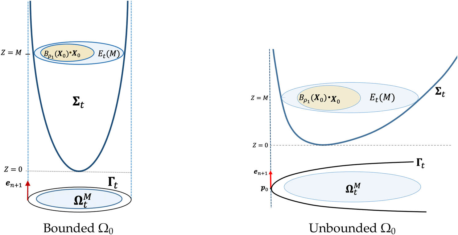
Case of a bounded domain.

Consider a bounded domain Ω t = π ( Σ t ) and Γ t j = π ( { X n + 1 = j } ∩ Σ t ) , j ∈ N . Fix a point p ∈ Γ t = ∂ ( π ( Σ t ) ) . Take a sufficiently small neighborhood around p so that one has graph representations for Γ t and Γ t j with graph functions w and w j , respectively, satisfying a monotone property that

(8.4) w ≤ w j + 1 ≤ w j .

Since w j converges pointwise to w and one has a uniform C 2 , α estimate for w j , independent of j , from Propositions 4.5 and 4.6, one has the same uniform C 2 , α estimate for w . Thus, the limit Γ t has C 2 , α regularity.

The regularity theory ensures that the evolution of Γ t is governed by the α -mean curvature flow. More precisely, the limit Γ t of the boundary Γ t z for the projection Ω t z of Σ t z as z → ∞ coincides with the solution of the coincides with the solution of the α -mean curvature flow whose initial submanifold of codimension two is Γ 0 . This shall be discussed in the following. Parametrizing hypersurfaces on S n with the standard metric g ¯ i j on the sphere since the second fundamental form has principle radii as its eigenvalues, i.e., h i j g ¯ j k = g i l ( h − 1 ) l k , one obtains

(8.5) ∂ S ∂ t = − ( g i j ( ∇ ¯ i ∇ ¯ j S + S g ¯ i j ) ) α = − ( h m i h k j g ¯ k m ∇ ¯ i ∇ ¯ j S + S ∣ A ∣ 2 ) α .

From Corollary 4.7 and Theorem 5.3, one has C 1,1 estimates for S and therefore C 2 , α estimates. Note that the unit normal vector ν z to Σ t on the level set { X ∈ Σ t : u = z } converges to the unit normal vector ν b = lim z → ∞ ν b z as z → ∞ , where ν b z is the unit normal vector to Γ t z . From (8.3), after rearranging the indices i , j , k , and m if necessary, one can have h 1 1 = λ 1 and conclude that H b ≔ lim z → ∞ ( λ 2 + ⋯ + λ n ) is the mean curvature of Γ t satisfying

(8.6) ∂ S ∂ t = − H b α , on S n − 1 × [ 0 , T * ) .

Therefore, one has a family of immersions x b : N n − 1 → R n , where N n − 1 is an ( n − 1 ) -dimensional complete Riemannian manifold and x b ( N ) = ∂ Ω t = Γ t satisfying

(8.7) ∂ ∂ t x b = − H b α ν b ,

where H b = lim z → ∞ ( λ 2 + ⋯ + λ n ) is the mean curvature of Γ t and ν b is the outward unit normal vector to Γ t . As discussed in Theorem 7.1, one has the long-time existence for Γ t , and therefore, x b is a solution of the α -mean curvature flow of codimension two in R n + 1 .

Lemma 8.1

Let T * and T b * be the maximal time for the flow of Σ t obtained in Theorem 7.1 and that of Γ t , respectively. Then, one has T * = T b * .

Proof of Lemma 8.1

To prove T * = T b * , we first suppose that T * < T b * . Denote by Ω ˆ t (resp. Γ ˆ t ) the solution of the α -mean curvature flow starting from Ω 0 (resp. Γ 0 ). Note that Σ t exists for t ∈ [ 0 , T * ) and Ω ˆ t exists for t ∈ [ 0 , T b * ) . From the previous discussion in (8.7), it follows that

(8.8) Ω t = π ( Σ t ) = Ω ˆ t , for 0 ≤ t < T * .

Also, there exists a ball B ρ 0 in Ω ˆ T * , where ρ 0 > 0 , due to the hypothesis T * < T b * . Using the convexity of Σ T * which follows from that of Σ t , it follows that Σ T * encloses a closed ( n + 1 ) -dimensional ball B n + 1 ( ρ 1 ) of radius ρ 1 . As in Theorem 7.1, a uniform bound for H follows from Lemma 4.2 and Proposition 4.5 so that one has bounds for the second derivatives, giving C 2 , α estimates for hypersurfaces Σ t up to t = T * . Using the short-time existence, where the details can be found in [7] and [13], the flow of Σ t can be extended beyond t = T * for a short time. This contradicts to the definition of T * , and one has T * ≥ T b * .

It remains to show that T * ≤ T b * . This follows from an argument similar to the one mentioned earlier. Suppose that T * > T b * . Then, there exists an ( n + 1 ) -dimensional ball inside the convex hull of Σ T b * . From (8.7), Ω T b * = π ( Σ T b * ) exists and contains an n -dimensional ball. Thus, the maximal time of Γ t is greater than T b * , yielding a contradiction to T b * being maximal. Therefore, T * = T b * as required.□

8.2 Unbounded domain Ω 0

We consider the case in which the initial projection Ω 0 = π ( Σ 0 ) is strictly convex, smooth, and unbounded. The cases of convex unbounded domains with corners or disconnected boundaries will be studied in the sequel. For an unbounded strictly convex domain Ω 0 , its boundary Γ 0 is a strictly convex graph on R n − 1 and remain so due to the convexity of Σ t . Note that Σ 0 z is compact for each z .

We now proceed as in Section 8.1 for a compact subset Ω 0 ∩ B R . Let x 0 * be the point on Ω 0 ∩ ∂ B R ⁄ 2 such that

(8.9) d ( x 0 * , Γ 0 ) = sup x ∈ Ω 0 ∩ ∂ B R ⁄ 2 d ( x , Γ 0 ) ,

where d ( x , Γ ) = inf y ∈ Γ ∣ x − y ∣ . As in Section 8.1, let X ( z 0 ) be the lowest point of Σ 0 , and write it as X ( z 0 ) = ( x ( z 0 ) , 0 ) . Then, let the point ( x 0 * , 0 ) be the origin O , and let X 0 * be the lift of x 0 * , i.e., x 0 * = π ( X 0 * ) . Then, there is a 2-plane Π θ through X 0 * spanned by e n + 1 and ( θ , 0 ) for some θ in the sphere S n − 1 . Denote by σ θ ( z ) the convex curve of Π θ ∩ Σ t z starting at X 0 * inside the cylinder ( Ω 0 ∩ B R ) × R + . Furthermore, let X ( z θ ) be the end point of σ θ ( z ) on Π θ . Then, for each θ in S n − 1 , p z θ = π ( X ( z θ ) ) is the point of Γ t z in θ -direction on the projected domain Ω t z , as shown in Figure 4. Let p ¯ θ = lim z → ∞ p z θ . Consider the following function ζ R for the points p z θ on Γ t z ∩ B R :

(8.10) ζ R ( z , θ ) ≔ ⟨ p ¯ θ − p z θ , θ ⟩ R n ,

where ⟨ ⋅ , ⋅ ⟩ R n is the standard inner product in R n . Then, as in (8.3), the smallest principal curvature λ 1 ( Σ t ) of Σ t converges to zero as z → ∞ .

Figure 4

Case of an unbounded domain.

Note that Γ t M ∩ B R ⁄ 3 is an approximation to the solution of the α -mean curvature flow and the higher derivatives of curvature are uniformly bounded on each Γ t M ∩ B R ⁄ 3 using the results in Sections 6 and 7. Then, as in the case of a bounded domain in Section 8.1, one can conclude that Γ t M ∩ B R ⁄ 3 smoothly converges to Γ t ∩ B R ⁄ 3 as M → ∞ . Finally, one has the α -mean curvature flow of codimension two satisfying (8.7).

From Theorem 1.3, one has an immediate corollary for two-dimensional hypersurfaces.

Corollary 8.2

Given a two-dimensional strictly convex complete non-compact smooth hypersurface over a strictly convex smooth domain as an initial hypersurface,

the solution of (1.1) exists for a finite time if the projection of the initial graph is bounded, and
the solution of (1.1) exists for all time if the projection of the initial graph is unbounded.

Proof

For ( i ) , Σ t is enclosed inside a round cylinder S R 0 1 × R , where S R 0 1 is a circle of radius R 0 enclosing Ω 0 , and by the comparison principle, the result easily follows. The case of ( i i ) can be seen from the one-dimensional case of the α -Gauss curvature flows in Theorem 1.1 of [4], i.e., the graphs evolving by the α -curve shortening flow exist for all time. Thus, Theorem 1.3, our main theorem, implies that solution of (1.1) defined over an unbounded domain exists for all time.□

Remark 8.3

In higher-dimensional cases, Corollary 8.2 may not hold. For example, consider any three-dimensional strictly convex graphical hypersurface defined over an unbounded strictly convex domain contained in a solid cylinder D 2 × R . Then, the projection of the hypersurface onto R 3 disappears in finite time, and so does the hypersurface.

Acknowledgments

The authors are enormously grateful to the referees for the detailed and helpful comments to improve the manuscript.

Funding information: H. Kang was supported by GIST Research Project grant funded by the GIST in 2025. K. Lee was supported by the Ministry of Education of the Republic of Korea and the National Research Foundation of Korea (RS-2025-00515707). T. Lee has been supported by the NRF grant funded by the Korea government (MSIT) (No. RS-2023-00211258).
Author contributions: All authors contributed equally to the preparation and the revision of the manuscript. All authors approved the final version of the manuscript.
Conflict of interest: The authors state no conflict of interest.

References

[1] B. Andrews, Contraction of convex hypersurfaces in Euclidean space, Calc. Var. PDE. 2 (1994), 151–171, https://doi.org/10.1007/BF01191340. Search in Google Scholar

[2] S. B. Angenent, P. Daskalopoulos, and N. Sesum, Dynamics of convex mean curvature flow, J. Reine Angew. Math. (Crelles Journal) (2025), https://doi.org/10.1515/crelle-2025-0029. Search in Google Scholar

[3] K. Choi and P. Daskalopoulos, The Qk flow on complete non-compact graphs, Calc. Var. PDE. 61 (2022), 73, https://doi.org/10.1007/s00526-021-02162-8. Search in Google Scholar

[4] K. Choi, P. Daskalopoulos, L. Kim, and K. A. Lee, The evolution of complete non-compact graphs by powers of Gauss curvature, J. reine angew. Math. (Crelles J.) 2019 (2019), no. 757, 131–158, https://doi.org/10.1515/crelle-2017-0032. Search in Google Scholar

[5] P. Daskalopoulos and M. Saez, Uniqueness of entire graphs evolving by mean curvature flow, J. reine angew. Math. (Crelles Journal) 796 (2023), 201–227, https://doi.org/10.1515/crelle-2022-0085. Search in Google Scholar

[6] K. Ecker and G. Huisken, Mean curvature evolution of entire graphs, Ann. Math. 130 (1989), 453–471, https://doi.org/10.2307/1971452. Search in Google Scholar

[7] K. Ecker and G. Huisken, Interior estimates for hypersurfaces moving by mean curvature, Invent. Math. 105 (1991), 547–569, https://doi.org/10.1007/BF01232278. Search in Google Scholar

[8] M. Franzen, Entire graphs evolving by powers of the mean curvature, 2011, http://arxiv.org/abs/1112.4359. Search in Google Scholar

[9] D. Gilbarg and N. Trudinger, Elliptic partial differential equations of second order, Classics in Mathematics, Springer-Verlag, Berlin, 2001. 10.1007/978-3-642-61798-0Search in Google Scholar

[10] G. Huisken, Flow by mean curvature of convex surfaces into spheres. J. Differ. Geom. 20 (1984), 237–266, https://doi.org/10.4310/jdg/1214438998. Search in Google Scholar

[11] S. Kim and K. Lee, Parabolic Harnack inequality of viscosity solutions on Riemannian manifolds. J. Funct. Anal. 267 (2014), no. 7, 2152–2198, https://doi.org/10.1016/j.jfa.2014.07.023. Search in Google Scholar

[12] N. V. Krylov and M. V. Safonov, A property of the solutions of parabolic equations with measurable coefficients. Math. USSR-Izvestiya 16 (1981), no. 1, 151–164, 10.1070/IM1981v016n01ABEH001283. Search in Google Scholar

[13] O. A. Ladyzhenskaya, V. A. Solonnikov, and N. N. Uralceva, Linear and Quasilinear Equations of Parabolic Type, Amer. Math. Soc, Providence, RI, 1968. Search in Google Scholar

[14] G. Li and Y. Lv, Evolution of complete noncompact graphs by powers of curvature function, 2019, http://arxiv.org/abs/1901.04099v1. Search in Google Scholar

[15] G. M. Liberman, Second Order Parabolic Differential Equations, World Scientific Publishing Co., Inc., River Edge, NJ, 1996. 10.1142/3302Search in Google Scholar

[16] C. Mantegazza, Lecture Notes on Mean Curvature Flow, Progress in Mathematics 290, Birkhauser, Basel, 2011. 10.1007/978-3-0348-0145-4Search in Google Scholar

[17] W. Maurer, Shadows of graphical mean curvature flow, Comm. Anal. Geom. 29 (2021), no. 1, 183–206, 10.48550/arXiv.1604.05238. Search in Google Scholar

[18] W. Maurer, Hα-flow of mean convex, complete graphical hypersurfaces, 2021, http://arxiv.org/abs/2104.00047. Search in Google Scholar

[19] M. Rupflin and O. C. Schnürer, Weak solutions to mean curvature flow respecting obstacles, Ann. Sc. Norm. Super. Pisa CL. Sci. 20 (2020), no. 5, 1429–1467, 10.2422/2036-2145.201708_005. Search in Google Scholar

[20] M. Sáez and O. C. Schnürer, Mean curvature flow without singularities, J. Differ. Geom. 97 (2014), 545–570, 10.4310/jdg/1406033979. Search in Google Scholar

[21] F. Schulze, Evolution of convex hypersurfaces by powers of the mean curvature, Math. Z. 251 (2005), 721–733, https://doi.org/10.1007/s00209-004-0721-5. Search in Google Scholar

[22] F. Schulze, Convexity estimates for flows by powers of the mean curvature, Ann. Sc. Norm. Super. Pisa Cl. Sci. 5 (2006), 261–277. 10.2422/2036-2145.2006.2.06Search in Google Scholar

[23] G. Tian and A. Wang, A priori estimates for fully nonlinear parabolic equations, Int. Math. Res. Not. 17 (2013), 3857–3877, https://doi.org/10.1093/imrn/rns169. Search in Google Scholar

[24] K. Tso, Deforming a hypersurface by its Gauss-Kronecker curvature, Comm. Pure. Appl. Math. 38 (1985), no. 6, 867–882, https://doi.org/10.1002/cpa.3160380615. Search in Google Scholar

[25] L. Wang, On the regularity theory of fully nonlinear equations: I, Comm. Pure. Appl. Math. 45 (1992), no. 1, 27–76, https://doi.org/10.1002/cpa.3160450103. Search in Google Scholar

[26] H. Wu, The spherical images of convex hypersurfaces, J. Differ. Geom. 9 (1974), 279–290, https://doi.org/10.4310/jdg/1214432294. Search in Google Scholar

[27] X. P. Zhu, Lectures on Mean Curvature Flows, Studies on Advanced Mathematics, vol. 32, AMS, Boston, 2002. 10.1090/amsip/032Search in Google Scholar

Received: 2023-12-27

Revised: 2024-12-29

Accepted: 2025-06-24

Published Online: 2025-08-20

This work is licensed under the Creative Commons Attribution 4.0 International License.

Articles in the same Issue

https://doi.org/10.1515/anona-2025-0101

Keywords for this article

mean curvature flow; graph

Creative Commons

BY 4.0