Blood flow analysis in narrow channel with activation energy and nonlinear thermal radiation
-
Anum Tanveer
 and
Zain Ul Abidin
and
Zain Ul Abidin

Abstract
Blood flow in narrow channels such as veins and arteries is the major topic of interest here. The Casson fluid with its shear-thinning attribute serves as the blood model. Owing to the arterial walls, the channel is configured curved in shape. The activation energy and nonlinear thermal radiation aspects are highlighted. The channel boundaries are flexible with peristaltic wave travelling along the channel. The mathematical description of the problem is developed under physical laws and then simplified using the lubrication technique. The obtained system is then sketched in graphs directly using the numerical scheme NDSolve in Mathematica software. The physical interpretation of parameters on axial velocity, temperature profile, concentration, and streamline pattern is discussed in the last section.
1 Introduction
The basic smallest quantity of energy needed by the reactants for a chemical reaction to arise is called activation energy. The term activation energy was first given by Svante Arrhenius, a Swedish scientist in 1989. A detailed review of activation energy was studied by Bestman [1]. Activation energy plays a significant role in the field of oil emulsion mechanics, geothermal or oil reservoir engineering, and chemical engineering. Presently, some studies have been made related to activation energy [2–12].
Due to outstanding features in the field of technical and industrial sciences, non-Newtonian fluids are primarily used in mathematical models for explaining realistic flow problems. One of these fluids, invented by Casson [13] in 1959, is known as the Casson fluid. He developed this model for printing ink oil suspensions. The Casson fluid model can also be used in other fluid models with alike properties, such as honey, jelly, and ketchup. The Casson fluid model can be used to characterise the blood flow in the capillary vessels due to the occurrence of fibrinogens, red corpuscles, and proteins [14]. The Casson fluid also plays an important role in blood dialysers and oxygenators. Some other useful studies relating to the Casson fluid flow are presented in refs. [15–21].
Peristalsis is one of the most important aspects of human physiology that can be seen in the human tabular functioning organs and blood flow in narrow arterial walls. Peristalsis is the relaxation and involuntary constriction of a canal that produces a wave to form, which forces the material to fall in an anterograde direction. It is a necessary feature of a number of engineering and biomedical sciences. Peristaltic flow is a type of fluid transport that occurs when a wave’s advanced area of shortening and development with a combination of the length of a distensible channel transports the fluid in the wave’s propagation direction. Initially, Latham [22] published a theoretical model of the peristaltic flow, and later, Shapiro et al. [23] confirmed it through its experiment. Further studies on the peristaltic flow can be seen in refs. [24–29].
Thermal radiation has an important application in heat exchangers, solar power plants, nuclear reactors, furnace design, power and solar technology, etc. Electromagnetic radiation causes radiative heat transfer. Radiation does not need a medium to work, but it is affected by factors such as temperature, surface properties, and geometric structure of the material absorbing or emitting heat. It is self-evident that when the temperature difference between two bodies is high or low, the radiation transmission between them is reduced. In industry, designing a structure with fluid flow and small temperature differences within a structure is laborious. Due to this laborious, researchers’ recently proposed nonlinear thermal radiation, which differs from linear thermal radiation in that it has an additional parameter. Refs. [30–32] cover some useful studies with nonlinear thermal radiation.
In the view of activation energy, the current work explores the peristaltic flow of the Casson fluid model in a curved channel. The phenomenon is modelled by utilising the equations of continuity, momentum, energy, and concentration. The physical outcomes of involved parameters on axial velocity, temperature variation, concentration, and streamline profile are discussed through graph using a numerical scheme NDSolve in MATHEMATICA software. The objectives of this research are discussed in the last section.
2 Mathematical problem
Here, we consider the incompressible Casson fluid flowing in a curved channel of half width
where
The following expression occurs in view of Ohm’s law:
The constitutive equations are given as follows:
Continuity equation:
Component of equations of momentum in axial and radial directions are as follows:
Equation of energy with viscous dissipation and nonlinear radiation effects reads:
Rosseland [33] gives the definition for nonlinear thermal radiation as follows:
Equation of concentration with activation energy reads:
The no-slip and flexible wall conditions can be written as follows:
In the aforementioned equations,
The rheological equation for the Casson fluid model is given by [34]:
where
where µ is the fluid viscosity, α is the Casson fluid parameter, and
The dimensionless variables are as follows:
where p is the pressure, Re the Reynolds number, T
1 the temperature at upper wall, ν the kinematic viscosity, C
1 the concentration at upper wall, H the Hartman number, k the radius of curvature, Pr the Prandtl number, δ the wave number, Br the Brinkman number, E
1
, E
2, and E
3 the elasticity parameters, Sc the Schmidt number, the amplitude ratio parameter, Ec the Eckert number, Rd the thermal radiation parameter, ϵ the ampltude ratio parameter, K
∗ the dimensionless reaction parameter, β the temperature difference parameter,
By implication of non-dimensional variables in the considered system under large wavelength
where
Eliminating the pressure term from Eqs. (19) and (20), we obtain
The dimensionless boundary conditions under the stream function are as follows:
Here,
The dimensionless wave shape is given by
3 Discussion
This section describes the effects of involved parameters on the peristaltic flow of the Casson fluid with activation energy, nonlinear thermal radiation, and viscous dissipation in a curved channel. Their behaviour on axial velocity u, temperature variation θ, concentration φ, and streamlines are physically discussed in this section.
3.1 Velocity profile
Here, we represent the graphical results of the Hartman number, the Casson fluid parameter, and elasticity parameter on the velocity profile. In Figure 1(a), we see that the increase in the values of Hartman number H reduces the velocity profile u. The magnetic field applied in the direction of flow behaves as a retarding force and is used to regulate the flow. This opposing character of the magnetic field is useful in treating diseases such as joint disorders, cancer, migraine headaches, and depression. Similar behaviour for the Casson fluid parameter α is shown in Figure 1(b). Figure 1(c) indicates that the velocity profile increases with wall elastic parameters E 1 and E 2 and reduces with damped constant E 3. The recorded outcomes are in comparison to blood vessels in which the blood velocity increases with elasticity E 1 or mass expansion per unit area E 2. However, damping E 3 increases the blood flow capacity and decreases the velocity within the channel. Similar results are observed in studies [11,12].
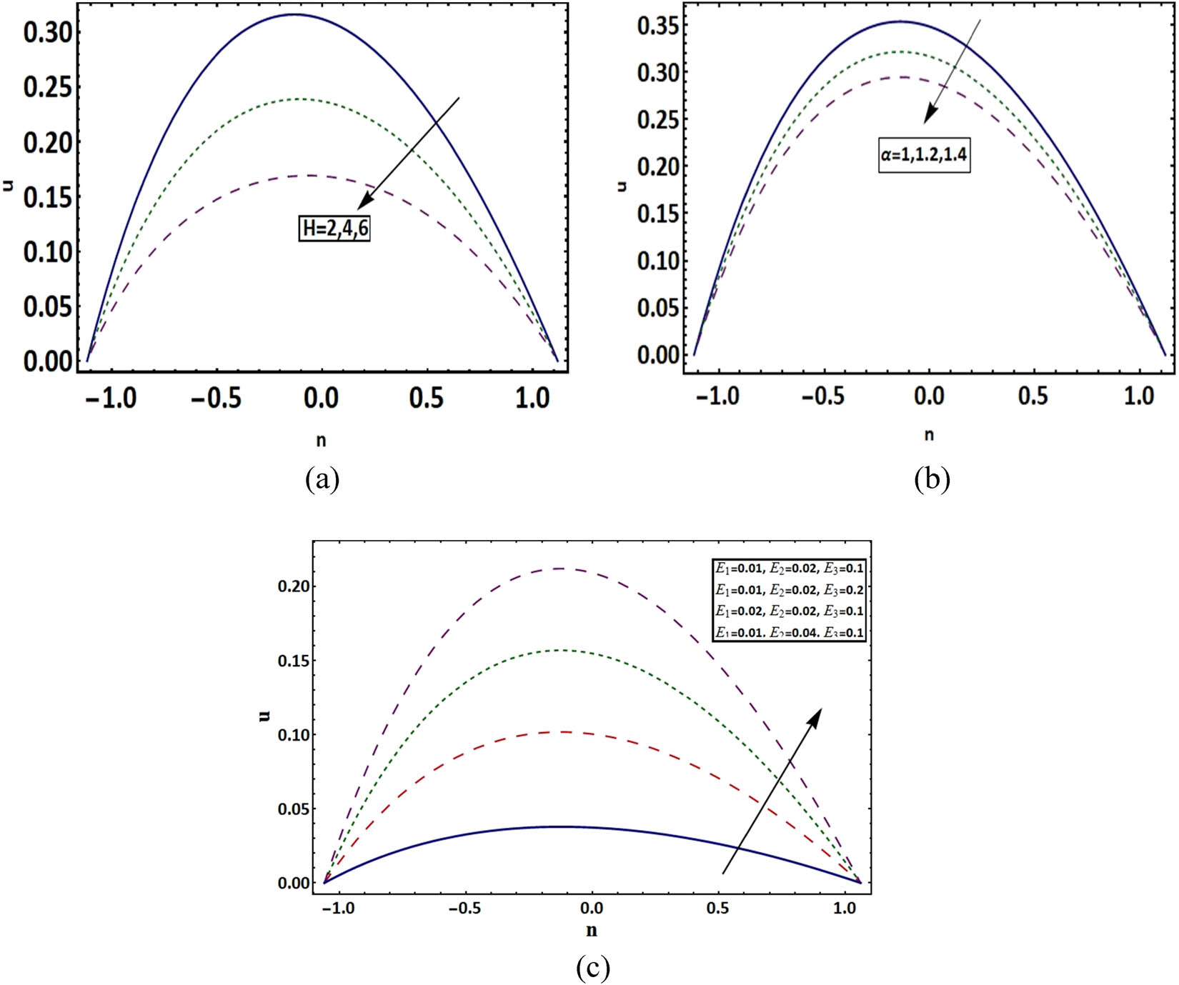
(a–c) Velocity profile at
3.2 Temperature profile
The behaviour of Hartmann number H on temperature θ is decreasing as shown in Figure 2(a). Since greater values of H produces a strong magnetic force that generates current in motor via fluid heat, the magnetic force acts as retarding force that induces temperature reduction. Similar behaviour is shown for the Casson fluid parameter α and radiation parameter Rd (see Figure 2(b) and (c)). Radiation converts thermal energy into electromagnetic energy, and it causes heat decay. In Figure 2(d), the temperature profile increases for increasing the values of the Brinkman number Br. In Figure 2(e), for increasing the value of Prandtl number Pr, a very small variation in temperature is detected. The results captured in Figure 2(f) display the dual response of temperature parameter θ w on θ. These results are considered to be very similar to refs. [11,12].

(a–f) Temperature profile at
3.3 Concentration profile
This section describes the concentration variation φ effected by fitted rate constant n, temperature difference parameter β, electrically conductivity σ, Schmidt number Sc, and activation energy E 4 (Figure 3(a)–(e)). Figure 3a shows that the concentration profile reduces with the increase in the value of Schmidt number Sc. The ratio of the momentum diffusion rate to the mass diffusion rate is mathematically expressed by Schmidt number Sc and the mass diffusion rate is low for larger Schmidt number Sc, which decreases concentration. Similar behaviour is captured for fitted rate constant n, temperature difference parameter β, and electrically conductivity σ (Figure 3(b)–(d)). The concentration profile increases with the increasing values of activation energy E 4 (Figure 3(e)). The modified Arrhenius function degrades as E 4 is increased. Eventually, this encourages reproductive chemical reactions, which result in an increase in concentration. The results are similar to the previous studies [11,12].
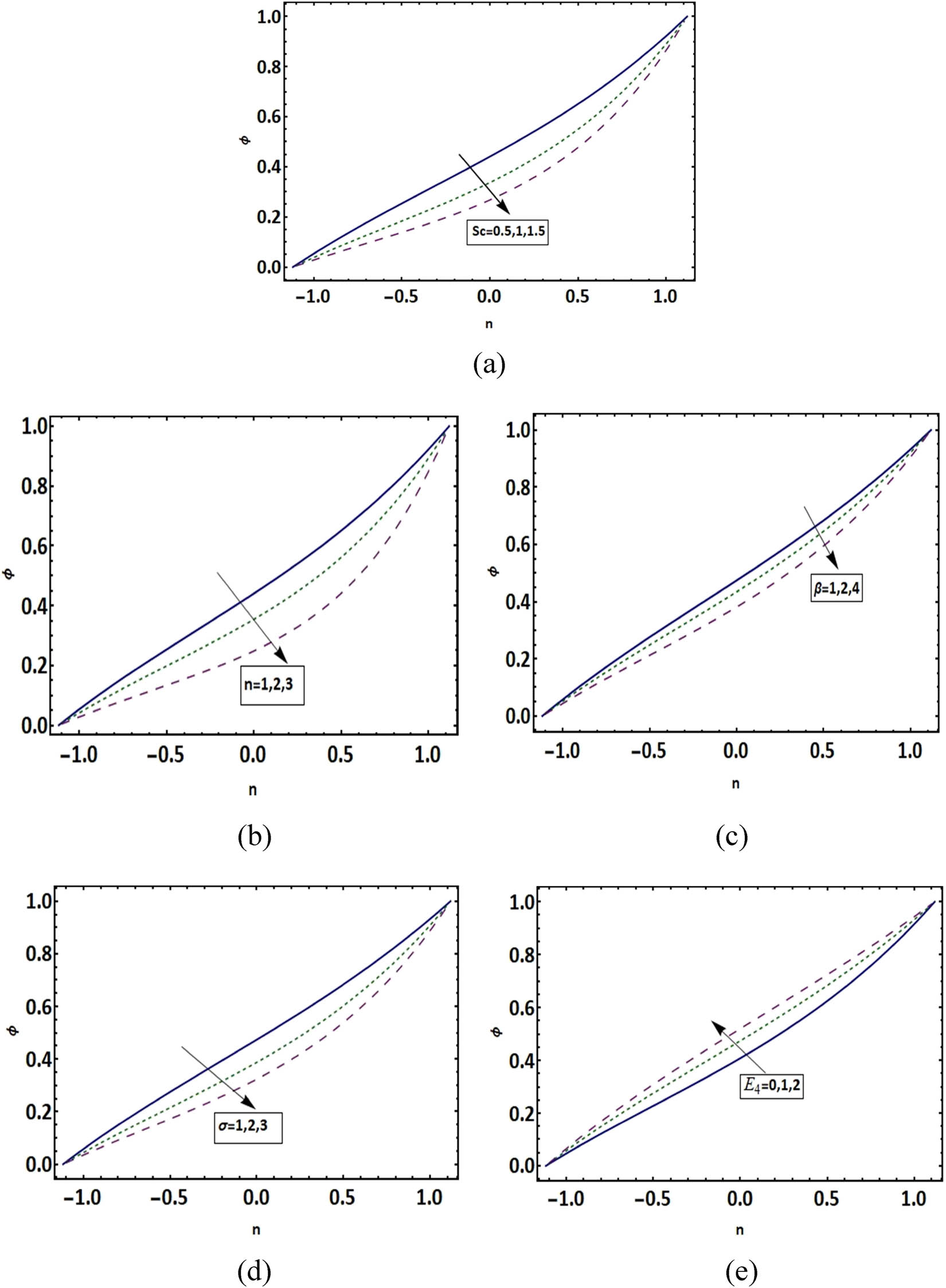
(a–e) Concentration profile at
3.4 Streamline profile
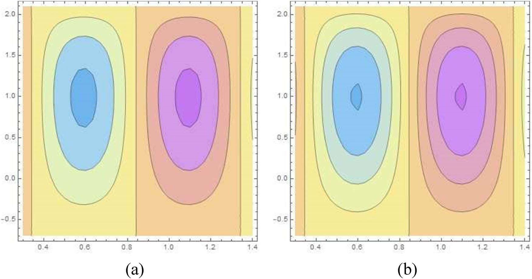
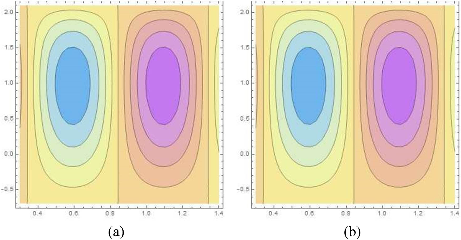
Figures 4–9(a) and (b) describe the streamlines for diverse values of the Casson fluid parameter α, elasticity parameters E 1, E 2, and E 3, and radius of curvature parameter k in curved channel. Figure 4(a) and (b) shows that an increment in the values of α causes a shrinking in the size of the bolus. Similar behaviour is captured for E 1 and E 2 (Figures 5, 6(a) and (b)). However, the bolus size enlarges for E 3, H, and k (Figures 7, 9(a) and (b)).

Streamlines for the Casson fluid parameter: (a)

Streamlines for elastic parameter
Streamlines for mass charactrising parameter

Streamlines for damping parameter
Streamlines for Hartman number H (a)

Streamlines for curvature parameter k (a)
4 Conclusions
In this article, the peristaltic flow of the Casson fluid in a curved channel is carried out for activation energy, nonlinear thermal radiation, and viscous dissipation. The main outcomes are as follows:
The reduction in flow velocity is noticed with the Hartman number H as it behaves as a retarding force to flow.
Behaviour of the Casson fluid parameter α on velocity and temperature profile is found to increase.
Thermal radiation Rd reduces the temperature profile, while the Brinkman number Br rises the temperature profile.
Concentration profile increases as we increase the effect of activation energy.
Reduction in φ is noticed with an increase in β, σ, Sc, and n.
The bolus shrinking is observed for an increase in α, E 1, and E 2. However, the bolus size enlarges for E 3, H, and k.
-
Funding information: The authors receive no specific funding for this research work.
-
Author contributions: AT conceived the presented idea. AT contributed in providing necessary guide in mathematical formation and its graphical description. ZUA developed the theory and performed the calculations. Both the authors contributed in finalizing the manuscript writing.
-
Conflict of interest: The authors declare no conflict of interest with anyone.
References
[1] Bestman AR. Natural convection boundary layer with suction and mass transfer in a porous medium. Int J Energy Res. 1990;14:389–96.10.1002/er.4440140403Search in Google Scholar
[2] Abbas SZ, Khan MI, Kadry S, Khan WA, Israr-Ur-Rehman M, Waqas M. Fully developed entropy optimized second order velocity slip MHD nanofluid flow with activation energy. Comput Methods Prog Biomed. 2020;190:105362.10.1016/j.cmpb.2020.105362Search in Google Scholar PubMed
[3] Javed M, Alderremy AA, Farooq M, Anjum A, Ahmad S, Malik MY. Analysis of activation energy and melting heat transfer in MHD flow with chemical reaction. Eur Phys J Plus. 2019;134:256.10.1140/epjp/i2019-12744-5Search in Google Scholar
[4] Shah Z, Kumam P, Deebani W. Radiative MHD Casson nanofluid flow with activation energy and chemical reaction over past nonlinearly stretching surface through entropy generation. Sci Rep. 2020;10:1–4.10.1038/s41598-020-61125-9Search in Google Scholar PubMed PubMed Central
[5] Khan SU, Waqas H, Shehzad SA, Imran M. Theoretical analysis of tangent hyperbolic nanoparticles with combined electrical MHD, activation energy and Wus slip features: a mathematical model. Phys Scr. 2019;14:125211.10.1088/1402-4896/ab399fSearch in Google Scholar
[6] Shahid A, Huang HL, Khalique CM, Bhatti MM. Numerical analysis of activation energy on MHD nanofluid flow with exponential temperature-dependent Viscosity past a porous plate. J Therm Anal Calorim. 2020;143:1–12.10.1007/s10973-020-10295-9Search in Google Scholar
[7] Dhlamini M, Kameswaran PK, Sibanda P, Motsa S, Mondal H. Activation energy and binary chemical reaction effects in mixed convective nano fluid flow with convective boundary condition. J Comput Des Eng. 2019;6:149.10.1016/j.jcde.2018.07.002Search in Google Scholar
[8] Majeed A, Noorib FM, Zeeshanc A, Mahmoodd T, Rehmane SU, Khan I. Analysis of activation energy in magnetohydrodynamic flow with chemical reaction and second order momentum slip model. Case Stud Therm Eng. 2018;12:765773.10.1016/j.csite.2018.10.007Search in Google Scholar
[9] Ahmad S, Nadeem S. Analysis of activation energy and its impact on hybrid nanofluid in the presence of Hall and ion slip currents. Appl Nanosci. 2020;10:5315–30.10.1007/s13204-020-01334-wSearch in Google Scholar
[10] Khan NS, Kumam P, Thounthong P. Second law analysis with effects of Arrhenius activation energy and binary chemical reaction on nanofluid flow. Sci Rep. 2020;10:1–16.10.1038/s41598-020-57802-4Search in Google Scholar PubMed PubMed Central
[11] Hayat T, Bibi F, Farooq S, Khan AA. Nonlinear radiative peristaltic flow of Jeffrey nanofluid with activation energy and modified Darcys law. J Braz Soc Mech Sci Eng. 2019;41:1–11.10.1007/s40430-019-1771-2Search in Google Scholar
[12] Abdelmalek Z, Mahanthesh B, Md Basir MF, Imtiaz M, Mackolil J, Khan NS, et al., Mixed radiated magneto Casson fluid flow with Arrhenius activation energy and Newtonian heating effects: Flow and sensitivity analysis. Alex Eng J. 2020;59:3991–4011.Search in Google Scholar
[13] Casson N. A flow equation for pigment oil suspensions of the printing ink type. In: Mill CC, editor. Rheology of Dispersed Systems. Oxford, UK: Pergamon Press; 1959. p. 84–104.Search in Google Scholar
[14] Alotta G, Bologna E, Failla G, Zingales M. A fractional approach to non-Newtonian blood rheology in capillary vessels. J Peridyn Nonlocal Model. 2019;1:8896.Search in Google Scholar
[15] Hamid M, Usman M, Khan ZH, Haq RU, Wang W. Heat transfer and flow analysis of Casson fluid enclosed in a partially heated trapezoidal cavity. Int Commun Heat Mass Transf. 2019;108:104284.10.1016/j.icheatmasstransfer.2019.104284Search in Google Scholar
[16] Kumam P, Shah S, Dawar A, Rasheed H, Islam S. Entropy generation in MHD radiative flow of CNTs Casson nanofuid in rotating channels with heat source/sink. Math Probl Eng. 2019;2019:9158093.10.1155/2019/9158093Search in Google Scholar
[17] Alotta G, Bologna E, Failla G, Zingales M. A fractional approach to non-Newtonian blood rheology in capillary vessels. J Peridyn Nonlocal Model. 2019;1:8896.10.1007/s42102-019-00007-9Search in Google Scholar
[18] Salahuddin T, Arshad M, Siddique N, Alqahtani AS, Malik MY. Thermophyical properties and internal energy change in Casson fluid flow along with activation energy. Ain Shams Eng J. 2020;11:1355–65.10.1016/j.asej.2020.02.011Search in Google Scholar
[19] Sheikh NA, Ching DLC, Khan I, Kumar D, Nisar KS. A new model of fractional Casson fluid based on generalized Ficks and Fouriers laws together with heat and mass transfer. Alex Eng J. 2020;59:2865–76.10.1016/j.aej.2019.12.023Search in Google Scholar
[20] Deebani W, Tassaddiq A, Shah Z, Dawar A, Ali F. Hall effect on radiative Casson fluid flow with chemical reaction on a rotating cone through entropy optimization. Entropy. 2020;22:480.10.3390/e22040480Search in Google Scholar PubMed PubMed Central
[21] Kumar KA, Sugunamma V, Sandeep N. Effect of thermal radiation on MHD Casson fluid flow over an exponentially stretching curved sheet. J Therm Anal Calorim. 2020;140:2377–85.10.1007/s10973-019-08977-0Search in Google Scholar
[22] Latham TW. Fluid motion in a peristaltic pump. MS thesis. Cambridge: Massachusetts Institute of Technology; 1966.Search in Google Scholar
[23] Shapiro AH, Jaffrin MY, Wienberg SL. Peristaltic pumping with long wavelengths at low Reynolds number. J Fluid Mech. 1969;37:799825.10.1017/S0022112069000899Search in Google Scholar
[24] Rashid M, Ansar K, Nadeem S. Effects of induced magnetic field for peristaltic flow of Williamson fluid in a curved channel. Phys A: Stat Mech Appl. 2020;296:123979.10.1016/j.physa.2019.123979Search in Google Scholar
[25] Javed M, Naz R. Peristaltic flow of a realistic fluid in a compliant channel. Phys A: Stat Mech Appl. 2020;551:123895.10.1016/j.physa.2019.123895Search in Google Scholar
[26] Khan LA, Raza M, Mir NA, Ellahi R. Effects of different shapes of nanoparticles on peristaltic flow of MHD nanofluids filled in an asymmetric channel. J Therm Anal Calorim. 2020;140:879–90.10.1007/s10973-019-08348-9Search in Google Scholar
[27] Riaz A, Khan SU-D, Zeeshan A, Khan SU, Hassan M, Muhammad T. Thermal analysis of peristaltic flow of nanosized particles within a curved channel with second-order partial slip and porous medium. J Therm Anal Calorim. 2021;143:1997–2009.10.1007/s10973-020-09454-9Search in Google Scholar
[28] Asha SK, Sunitah G. Mixed convection peristaltic flow of a eyring-powell nanofluid with magnetic field in a non-uniform channel. J Appl Math Comput. 2018;2:332334.10.26855/jamc.2018.08.003Search in Google Scholar
[29] Fusi L, Farina A. Peristaltic axisymmetric flow of a Bingham fluid. J Appl Math Comput. 2018;320:1–15.10.1016/j.amc.2017.09.017Search in Google Scholar
[30] Rashid M, Khan MI, Hayat T, Khan MI, Alsaedi A. Entropy generation in flow of ferromagnetic liquid with nonlinear radiation and slip condition. J Mol Liq. 2019;276:441–52.10.1016/j.molliq.2018.11.148Search in Google Scholar
[31] Hosseinzadeh Kh, Gholinia M, Jafari B, Ghanbarpour A, Olfian H, Ganji DD. Nonlinear thermal radiation and chemical reaction effects on Maxwell fluid flow with convectively heated plate in a porous medium. Heat Transfer Asian Res. 2019;48:744–59.10.1002/htj.21404Search in Google Scholar
[32] Ramzan M, Rafiq A, Chung JD, Kadry S, Chu Y. Nanofluid flow with autocatalytic chemical reaction over a curved surface with nonlinear thermal radiation and slip condition. Sci Rep. 2020;10:1–13.10.1038/s41598-020-73142-9Search in Google Scholar PubMed PubMed Central
[33] Rosseland S. Astrophysik und atom theoretische grundlagen. Berlin Heidelberg, Germany: Springer-Verlag; 1931. p. 41–4. (in German)Search in Google Scholar
[34] Abdelmalek Z, Mahanthesh B, Basir MdFMd, Imtiaz M, Mackolil J, Khan NS, et al. Mixed radiated magneto Casson fluid flow with Arrhenius activation energy and Newtonian heating effects: Flow and sensitivity analysis. Alex Eng J. 2020;59:3991–4011.10.1016/j.aej.2020.07.006Search in Google Scholar
© 2023 the author(s), published by De Gruyter
This work is licensed under the Creative Commons Attribution 4.0 International License.
Articles in the same Issue
- Research Articles
- The mechanical properties of lightweight (volcanic pumice) concrete containing fibers with exposure to high temperatures
- Experimental investigation on the influence of partially stabilised nano-ZrO2 on the properties of prepared clay-based refractory mortar
- Investigation of cycloaliphatic amine-cured bisphenol-A epoxy resin under quenching treatment and the effect on its carbon fiber composite lamination strength
- Influence on compressive and tensile strength properties of fiber-reinforced concrete using polypropylene, jute, and coir fiber
- Estimation of uniaxial compressive and indirect tensile strengths of intact rock from Schmidt hammer rebound number
- Effect of calcined diatomaceous earth, polypropylene fiber, and glass fiber on the mechanical properties of ultra-high-performance fiber-reinforced concrete
- Analysis of the tensile and bending strengths of the joints of “Gigantochloa apus” bamboo composite laminated boards with epoxy resin matrix
- Performance analysis of subgrade in asphaltic rail track design and Indonesia’s existing ballasted track
- Utilization of hybrid fibers in different types of concrete and their activity
- Validated three-dimensional finite element modeling for static behavior of RC tapered columns
- Mechanical properties and durability of ultra-high-performance concrete with calcined diatomaceous earth as cement replacement
- Characterization of rutting resistance of warm-modified asphalt mixtures tested in a dynamic shear rheometer
- Microstructural characteristics and mechanical properties of rotary friction-welded dissimilar AISI 431 steel/AISI 1018 steel joints
- Wear performance analysis of B4C and graphene particles reinforced Al–Cu alloy based composites using Taguchi method
- Connective and magnetic effects in a curved wavy channel with nanoparticles under different waveforms
- Development of AHP-embedded Deng’s hybrid MCDM model in micro-EDM using carbon-coated electrode
- Characterization of wear and fatigue behavior of aluminum piston alloy using alumina nanoparticles
- Evaluation of mechanical properties of fiber-reinforced syntactic foam thermoset composites: A robust artificial intelligence modeling approach for improved accuracy with little datasets
- Assessment of the beam configuration effects on designed beam–column connection structures using FE methodology based on experimental benchmarking
- Influence of graphene coating in electrical discharge machining with an aluminum electrode
- A novel fiberglass-reinforced polyurethane elastomer as the core sandwich material of the ship–plate system
- Seismic monitoring of strength in stabilized foundations by P-wave reflection and downhole geophysical logging for drill borehole core
- Blood flow analysis in narrow channel with activation energy and nonlinear thermal radiation
- Investigation of machining characterization of solar material on WEDM process through response surface methodology
- High-temperature oxidation and hot corrosion behavior of the Inconel 738LC coating with and without Al2O3-CNTs
- Influence of flexoelectric effect on the bending rigidity of a Timoshenko graphene-reinforced nanorod
- An analysis of longitudinal residual stresses in EN AW-5083 alloy strips as a function of cold-rolling process parameters
- Assessment of the OTEC cold water pipe design under bending loading: A benchmarking and parametric study using finite element approach
- A theoretical study of mechanical source in a hygrothermoelastic medium with an overlying non-viscous fluid
- An atomistic study on the strain rate and temperature dependences of the plastic deformation Cu–Au core–shell nanowires: On the role of dislocations
- Effect of lightweight expanded clay aggregate as partial replacement of coarse aggregate on the mechanical properties of fire-exposed concrete
- Utilization of nanoparticles and waste materials in cement mortars
- Investigation of the ability of steel plate shear walls against designed cyclic loadings: Benchmarking and parametric study
- Effect of truck and train loading on permanent deformation and fatigue cracking behavior of asphalt concrete in flexible pavement highway and asphaltic overlayment track
- The impact of zirconia nanoparticles on the mechanical characteristics of 7075 aluminum alloy
- Investigation of the performance of integrated intelligent models to predict the roughness of Ti6Al4V end-milled surface with uncoated cutting tool
- Low-temperature relaxation of various samarium phosphate glasses
- Disposal of demolished waste as partial fine aggregate replacement in roller-compacted concrete
- Review Articles
- Assessment of eggshell-based material as a green-composite filler: Project milestones and future potential as an engineering material
- Effect of post-processing treatments on mechanical performance of cold spray coating – an overview
- Internal curing of ultra-high-performance concrete: A comprehensive overview
- Special Issue: Sustainability and Development in Civil Engineering - Part II
- Behavior of circular skirted footing on gypseous soil subjected to water infiltration
- Numerical analysis of slopes treated by nano-materials
- Soil–water characteristic curve of unsaturated collapsible soils
- A new sand raining technique to reconstitute large sand specimens
- Groundwater flow modeling and hydraulic assessment of Al-Ruhbah region, Iraq
- Proposing an inflatable rubber dam on the Tidal Shatt Al-Arab River, Southern Iraq
- Sustainable high-strength lightweight concrete with pumice stone and sugar molasses
- Transient response and performance of prestressed concrete deep T-beams with large web openings under impact loading
- Shear transfer strength estimation of concrete elements using generalized artificial neural network models
- Simulation and assessment of water supply network for specified districts at Najaf Governorate
- Comparison between cement and chemically improved sandy soil by column models using low-pressure injection laboratory setup
- Alteration of physicochemical properties of tap water passing through different intensities of magnetic field
- Numerical analysis of reinforced concrete beams subjected to impact loads
- The peristaltic flow for Carreau fluid through an elastic channel
- Efficiency of CFRP torsional strengthening technique for L-shaped spandrel reinforced concrete beams
- Numerical modeling of connected piled raft foundation under seismic loading in layered soils
- Predicting the performance of retaining structure under seismic loads by PLAXIS software
- Effect of surcharge load location on the behavior of cantilever retaining wall
- Shear strength behavior of organic soils treated with fly ash and fly ash-based geopolymer
- Dynamic response of a two-story steel structure subjected to earthquake excitation by using deterministic and nondeterministic approaches
- Nonlinear-finite-element analysis of reactive powder concrete columns subjected to eccentric compressive load
- An experimental study of the effect of lateral static load on cyclic response of pile group in sandy soil