Mixing Behaviors of Jets in Cross-Flow for Heat Recovery of Partial Oxidation Process

2.1 Experimental setup

The JICF mixing apparatus was made of transparent polymethyl methacrylate with four jets equally spanned around the main pipe. The internal diameter of the jet channel (D) was 50 mm, and the internal diameter of the main channel was 2D, as shown in Figure 1. The jet inlets were introduced 20D away from the inlet of the mainstream in order to ensure full development of the turbulent flows. The length of the main pipe downstream of the jet inlets was 12D, as shown in Figure 1. The angles between the mainstream and jets were θ=90° and 120°. The four jets configuration was selected according to the correlation proposed by Holdeman (1993) for JICF:

where n is the number of jets, the empirical constant C is 2.5, and VR is the velocity ratio of jet to mainstream. ρ_m and ρ_j are the densities of mainstream and jet, which are equal to each other in our experiments.

Air was used as the fluid for both the mainstream and jets. The mixing behavior was measured by the gas tracing method. Methane was used as the tracing gas and was added to the mainstream. The axial and radial profiles of the methane concentration were measured by sampling and gas chromatography with flame ionization detector (FID). The concentration of methane added to the mainstream was 500 PPM. Calibrations showed that the minimum concentration of methane that could be detected by FID was 2.5 PPM. Therefore the methane concentrations could be measured with a good accuracy.

2.2 Measuring method

Several sampling ports with a diameter of 5 mm were mounted on the wall of the mixing apparatus, through which invasive sampling was accomplished. The sampling tube with an internal diameter of 2 mm was engraved with precise scale for accurate sampling position. The tube was connected to a sampling pump. The sucking flux of the pump was 0.1 L/min, which was small enough to eliminate the deviation of sampling location in invasive measurement. The gas sample was gathered in a gas sampling bag of 0.5 L, which allowed the measurement of the time-averaged concentration.

A gas chromatograph GC-7900 with FID detector was used to measure the methane concentration of the samples. A good linear relationship between the methane concentration and the methane peak area detected by FID was obtained by calibrations for methane concentration from 2.5 to 500 PPM, as shown in Figure 2. By fitting the calibration results, the following relationship was obtained.

where S is the peak area of methane in μV·s and f_methane is the volume fraction of methane in PPM.

Figure 1:

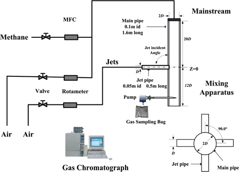
Schematic diagram of the experimental apparatus.

Figure 2:

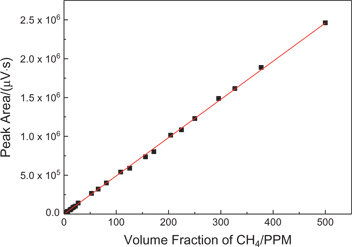
Relationship between volume fraction of methane and peak area.

3.1 Model description

The steady-state 3D simulations were performed with ANSYS FLUENT. The incompressible, dimensionless form of the Reynolds-averaged governing equations for continuity and momentum in Cartesian coordinates can be written as:

Although no difference exists between the simulation results of compressible and incompressible Navier-Stokes equations under the conditions of our experiments, i. e. relatively low gas velocity and no temperature difference between the jets and mainstream, the compressible form is used in consideration that the model will be further used to simulate the quenching process, in which high gas velocities and a large temperature gradient are involved and the compressible form is needed to predict correct results. The k-ε turbulence model was used because both the computational efficiency and accuracy are acceptable for simulation of industrial apparatus. The Boussinesq approximation was used to express the Reynolds stress term (Wilcox 1993):

where μt is the turbulent viscosity, k is the turbulent kinetic energy, and δ_ij is the Kronecker delta. Although k-ε model performs very well in many JICF cases (Hwang and Chiang 1995; Karvin and Ahlstedt 2005; Kartaev et al. 2014, 2015), it should be noted that Boussinesq hypothesis assumes turbulent viscosity is an isotropic scalar quantity, which is not strictly true.

In the k-ε model, the rate of dissipation ε is introduced and μt is expressed as the function of k and ε:

In the standard high Reynolds k-ε model, k and ε are determined from the following two transport equations:

The default values of the empirical constants in FLUENT are those recommended by Lauder and Spalding (1972), i. e.: C1ε=1.44, C2ε=1.92, Cμ=0.09, σk=1.0, σε=1.3. Those default values were used in this work. The transport equation for k is derived from exact equations. However, the transport equation for ε in the standard k-ε model is derived using physical reasoning, which relies on phenomenological considerations and empiricism. The dissipation of turbulence kinetic energy is essentially a second-rank tensor but in the k-ε model it is assumed to be locally isotropic, meaning that small-scale behaviors are independent of direction.

In the realizable k-ε model, the transport equation for k is the same as eq. (7); while the transport equation for ε is as follows:

where C1=max(0.43,ηη+5), η=Skε, S=2Sij. The mean strain rate is Sij=12∂uj∂xi+∂ui∂xj. The transport equation for ε in the realizable k-ε model is derived from an exact equation for the transport of the mean-square vorticity fluctuation, thus it satisfies mathematical constraints on Reynold stresses and it is consistent with the physics of turbulent flows.

The eddy viscosity μt in the realizable k-ε model is still based on eq. (6). However, C_μ is no longer a constant. Instead, it is a function of the mean strain and rotation rates, the angular velocity of system rotation as well as the turbulence fields. Further details can be seen in Fluent 6.3 user’s guide (2006). In comparison, the C_μ is only a function of strain rate in the RNG k-ε model, while in the standard k-ε model it is a constant. The realizable k-ε model has been validated for a wide range of flows and has been found to be substantially better than the standard k-ε model (Kim, Choudhury, and Patel 1997; Shih et al. 1995). The application of realizable k-ε model in the JICF also shows accurate predictions compared to experimental data (Li, Huai, and Qian 2012; Kartaev et al. 2014, 2015).

A steady segregated solver with implicit formulation was used. The Species Transport Model was used to simulate the mixing of air and methane. Considering that the k-ε models are primarily valid for the flow in a region far from walls, the Non-Equilibrium Wall Functions were used to model the flow in the near-wall region.

The unstructured tetrahedral mesh was used. A second-order upwind discretization scheme was used for all the governing equations, and the PRESTO! algorithm was used for pressure discretization. The SIMPLE algorithm was used for the pressure-velocity coupling and the relaxation factors were default values which showed a good convergence. The convergence criteria for velocity, turbulent kinetic energy, turbulence dissipation rate, energy equation, air concentration and methane concentration are 10^–5, 10^–5, 10^–5, 10^–7, 10^–6 and 10^–6, respectively.

3.2 Boundary conditions

The boundary conditions of the inlets were set based on the measurement of velocity, temperature and composition, except that the turbulent intensity was calculated using the equation given by Fluent 6.3 user’s guide (2006):

The calculation results for mainstream inlet (Re_m= 3.13×10⁴) and jet inlets (Re_j=1.57×10⁴) are 4.34 % and 4.73 %, respectively. Both of them are around 5 %; thus 5 % was used as the inlet turbulent intensity. It should be noticed that eq. (10) is only suitable for the core zone of fully developed turbulent flow in a smooth pipe. If the turbulent flow is not fully developed, the turbulent intensity should be smaller than the calculation result; while if the flow is disturbed, the turbulent intensity should be larger than the calculation result. The boundary conditions used in the calculations are listed in Table 1.

3.3 Mesh independence test

In order for the mesh independence test, five unstructured tetrahedral meshes of 10, 8, 6, 4 and 3 mm were investigated. A case of JICF with Re_m=3.13×10⁴ and VR=1 was simulated using the standard k-ε model. Figure 3 shows the influence of the grids on the simulated axial profiles of the methane mole fraction at different radial positions. The result of 4 mm mesh is very close to that of 3 mm mesh; therefore the 4 mm mesh was used for subsequent simulations. Prism layers were created in order to meet the requirement of wall Y⁺ when using the wall function.

Figure 3:

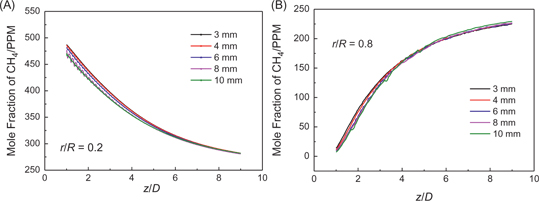
Effect of grid size on simulated axial profiles of methane fraction at (A) r/R=0.2 and (B) r/R=0.8.

3.4 Definition of mixedness

The intensity of segregation defined by Danckwerts (1952) was used to describe the mixedness of the mainstream and jets as follows:

where fA‾ and fB‾ are the average volume fraction of species A and B, respectively, and σfA is the standard deviation of f_A. According to eq. (11), the mixedness I_s equals to 0 when the two streams A and B are completely mixed, and equals to 1 when A and B are completely separated. A smaller I_s stands for a better mixing.

Some researchers (Kroll, Sowa, and Samuelsen 2000; Urson, Lightstone, and Thomson 2001) use the sample standard deviation s instead of standard deviation σ to calculate I_s. The definition of s is:

where A=∑ai is the cross-section area, f_i is the volume fraction measured at position i, and f‾ is the cross-sectional averaged value of f.

Strictly speaking, the intensity of segregation describes the unmixedness of mixing because normally the mixedness should be 1 when mixing is complete. Therefore, Fuller et al. (1998) use 1−I_s to describe the mixedness and a complete mixing is achieved when 1−I_s equals to 1. However, a drawback still exists because the variables mentioned above merely reflect the overall mixing effect but could not reflect the local mixing behavior. Considering that the spatial distribution of mixedness is very important to study the JICF for quenching in the POX process, the local mixedness η was defined in this work to describe the local mixing:

where fA∗ and fB∗ respectively represent the mole fraction of A and B when mixing is complete. When A and B are completely mixed, η=1; when A and B are completely separated, η=0. The cross-sectional averaged mixedness ηˉ can be calculated by the area-weighted method as follows:

where A is the cross-section area, a_i and η_i are respectively the cross-section area and mixedness of cell i. The mixedness for every cell and the cross-sectional averaged mixedness were calculated using user defined functions (UDF) and area-weighted average commands in FLUENT.

4.1 Experimental results and model validation

4.1.1 Effects of sucking and intrusion on measurements

Before the measurements, the effects of sucking flux and invasive measurements on experimental data were checked. Firstly an experiment was conducted to check the effect of sucking flux on the concentration measurements. Figure 4 shows the experimental data measured at different sucking fluxes at r/R=0 and z/D=4. It can be seen that the measured results become independent of the sucking flux when the sucking flux is smaller than 0.15 L·min^–1; therefore a sucking flux of 0.1 L·min^–1 is used, which is small enough to eliminate the deviation caused by sucking flow.

Figure 4:

Effect of sucking flux on concentration measurements at r/R=0, z/D=4 (θ=90°, Re_m=3.13×10⁴, VR=1).

Furthermore, the effect of invasive measurement on the experimental data was analyzed by CFD simulations. The simulation domain is the same as the mixing apparatus except that a sampling tube is placed in the mixing apparatus. The top of the sampling tube is set at r/R=0 and z/D=4 and it is simulated as a pressure-outlet. The lateral surface of the sampling tube is simulated as wall. With a sucking flux of 0.1 L·min^–1 and an internal diameter of 2 mm, the velocity component along the sampling tube is calculated to be 0.53 m·s^–1. By adjusting the pressure at the pressure-outlet of the sampling tube, the velocity component mentioned above is achieved; thus the invasive measurement is simulated. The simulated methane mole fraction at r/R=0 and z/D=4 is 1.5 PPM higher than the simulated methane mole fraction without sampling tube in the mixing apparatus. This difference is smaller than the standard deviation of the measured methane mole fraction at this sampling point (8 PPM). Thus the sampling tube would not cause a significant deviation of measurements.

4.1.2 Effect of turbulence models and model parameters

The simulation results with different k-ε models were firstly compared with the experimental data for model validation. Each sampling point was measured three times and the standard deviation of each point is shown in Figures. It can be seen that most of the standard deviations are within ±8 PPM, showing a good reliability of the experimental data. Figure 5 shows that the mixing rates predicted by the standard k-ε model and realizable k-ε model are much larger than that predicted by the RNG k-ε model. Among these three k-ε models, the realizable k-ε model has the best agreement with the experimental data. The main reason is that the realizable k-ε model is more suitable for high Reynolds number flow, rotational flow and pipe flow, and in this work the Reynolds number in the mixing zone is higher than 60000, which is large enough to use the high Re turbulent models.

Figure 5:

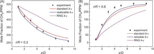
Comparison of axial methane mole fraction profiles of measurements and simulations with different k-ε models at (A) r/R=0.2 and (B) r/R=0.6 (Re_m=3.13×10⁴, VR=1, I=10 %).

With the realizable k-ε model, the effect of model parameters was further studied to improve the predictions. The primary value of inlet turbulent intensity used in the simulation was 5 %, which was estimated by eq. (10). Figure 6 shows that the simulated mixing with 5% inlet turbulent intensity is less intensive than the experimental results. The common approaches to enhance the mixing in simulations include increasing the inlet turbulent intensity and changing the value of the turbulent Schmidt number (Galezzo et al. 2011). The former approach was used since the turbulent intensity should be higher than the calculated value using eq. (10), as in our experiments both the mainstream and jets flowed through bellow tubes before entering the mixing apparatus. The axial profiles of the methane mole fraction simulated with inlet turbulent intensity of 5 %, 10 % and 15 % were compared. Figure 6 shows that the simulation results with inlet turbulent intensity of 10 % agree better with experimental data. The results also show that with the increase of turbulent intensity, the mixing between the mainstream and jets becomes more intensive. However, it is difficult to judge the value of inlet turbulent intensity only based on the simulation results and further measurements of inlet velocity fluctuation are needed.

Figure 6:

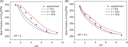
Comparison of measured and simulated axial profiles of methane fraction with different inlet turbulent intensities at (A) r/R=0 and (B) r/R=0.2 (Re_m =3.13×10⁴, VR=1, realizable k-ε model).

4.1.3 Model validation with different VR, θ and Re_m

The model and parameters were further validated by comparing simulation results with experimental data measured at different VR, θ and Re_m. Figure 7(A) and 7(B) show the comparison of the measured and simulated axial profiles of methane mole fraction at different radical positions with VR of 1 and 1.8. As we can see, the overall agreement of the simulations and experiments is satisfactory, confirming that using the realizable k-ε model is a computational efficient way to predict the mixing in JICF in the present work.

Figure 7:

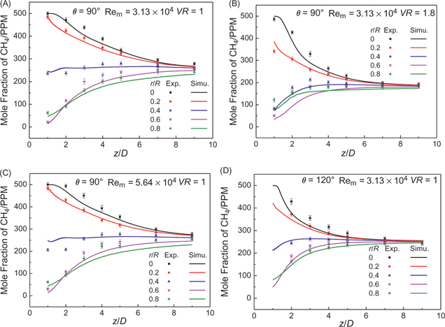
Comparison of measured and simulated axial methane mole fraction profiles at different radical positions for: (A) θ=90°, Re_m=3.13×10⁴ and VR=1, (B) θ=90°, Re_m =3.13×10⁴ and VR=1.8, (C) θ=90°, Re_m=5.64×10⁴ and VR=1 and (D) θ=120°, Re_m=3.13×10⁴ and VR=1.

Further study on the effect of gas velocity on mixing is needed because the Reynolds number of mainstream of experiments mentioned above is only 3.13×10⁴, while a Reynolds number of 3.13×10⁵–6.26×10⁵ will be used in the syngas quenching process. Limited by the flux of Roots blower in our lab, the highest Reynolds number of the mainstream could be achieved was 5.64×10⁴. Figure 7(C) shows the measured and simulated methane concentration profiles at Re_m=5.64×10⁴ and VR=1, which are quite like the profiles at Re_m=3.13×10⁴ and VR=1 shown in Figure 7(A). The good agreement between experimental and simulation data at both Re_m=3.13×10⁴ and Re_m=5.64×10⁴ confirms that the simulation results by realizable k-ε model could be used to study the effect of gas velocities.

A mixing apparatus with jet incident angle θ=120° was also built for further model validation. Figure 7(D) shows the comparison of the measured and simulated axial profiles at θ=120° and VR=1. The overall agreement of the simulations and experiments is acceptable, indicating that the realizable k-ε model has good predictions of the effect of jet incident angles on the mixing behaviors.

Although Figure 7 illustrates that the realizable k-ε model is able to predict concentration profiles in JICF, the agreement of the predicted and measured concentrations at the leeward side of the jets (i. e. r/R=0.6 and 0.8) is not as good as that at the windward side of the jets (i. e. r/R=0 and 0.2) in all four conditions shown in Figure 7. This phenomenon is also confirmed by Galeazzo et al. (2011). The reason for deviation of the simulations at the leeward side is because the simulations using k-ε model predict lower levels of Reynolds flux than the measurements. Consequently, the mixing at the leeward side of jets in measurements is more intensive than that in simulations.

4.2 Effect of velocity ratio

The gas densities of the mainstream and jets were kept constant in this work, thus the momentum-flux ratio J was proportional to the square of velocity ratio VR. Figure 7(A) and 7(B) show that with the increase of velocity ratio, the radial profile of the methane concentration becomes more uniform, indicating the mixing is enhanced.

Figure 8 shows the pseudo-color image of the spatial distribution of methane concentration in the plane through the central lines of the mainstream and jets. With the increase of VR, the jets penetrate deeper in the mainstream. No over-penetration is observed in the VR range of 1–1.8, and a further simulation with VR of 3 still shows no over-penetration. This indicates we can simply use the value of mixedness to optimize mixing in the VR range of 1–3 since in this case the mixing effect would monotonically change with the mixedness. It should be noted that Holdeman et al. (1997) and Holdeman, Liscinsky, and Bain (1999) found that if the VR was big enough to cause over-penetration, lower intensity of segregation (higher mixedness) could be obtained but actually over-penetration did cause an unfavorable effect on mixing.

Figure 8:

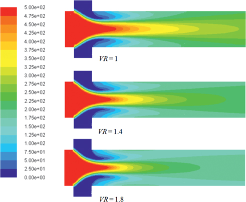
Comparison of spatial distributions of methane concentration (in PPM) at different VR values (θ=90°).

Figure 9 shows the pseudo-color image of the profile of local mixedness η in the plane through the central lines of the mainstream and jets. The results show that the jets initially mix with the mainstream at the windward side, and then the mixing zone expands to the near-wall region and the mainstream center. The increase of the velocity ratio VR enhances the jet penetration and reduces the length of unmixed core of mainstream, thus enhances the mixing. The ratio of velocities also significantly affects the profile of the cross-sectional averaged mixedness ηˉ. In addition, this effect strongly depends on the jet incident angle, as discussed later in Section 4.3.

Figure 9:

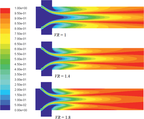
Comparison of spatial distributions of η at different VR values (θ=90°).

4.3 Effect of jet incident angle

The agreement between simulations and experiments allowed us to use the simulation results for studying the η spatial distribution. Figure 10 shows the cross-sectional averaged mixedness ηˉ at different axial positions with different VR and jet incident angles. Similar to the θ=90° configuration, the θ=120° configuration shows enhanced mixing with the increase of velocity ratio. Moreover, the ηˉ value in the θ=120° configuration is higher than that in the θ=90° for the same velocity ratio, indicating that the mixing can be enhanced by adjusting the jet incident angle.

Figure 10:

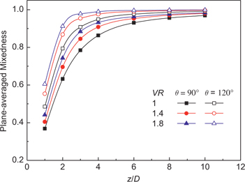
Effect of θ on cross-sectional averaged mixedness at different VR values.

Compared with the mixedness at the outlet, the mixing in the first few milliseconds, namely the initial mixing is more important for syngas quenching process to avoid acetylene consumption. An incident angle larger than 90° provides a velocity component against the mainstream, and the jets are more intensively sheared and broken up by the mainstream, thus the initial mixing is more rapid. However, because the velocity component perpendicular to the mainstream is smaller at a larger jet incident angle for the same jet inlet velocity, an inappropriate jet incident angle will lead to a decreased mixing efficiency at the main channel center. The plane at z/D=2 was selected and the cross-sectional averaged mixedness ηˉ was studied as a function of the velocity ratio VR and jet incident angle θ. The results are shown in Figure 11. It can be seen that at a small jet incident angle, the mixedness ηˉ monotonically increases with increasing velocity ratio in the VR range of 1–3. However, the tendency becomes different at larger jet incident angles. At jet incident angles larger than 120°, the mixedness ηˉ first increases and then decreases with the increase of velocity ratio, and the optimized velocity ratio is in the range of 1.8–2.4. Figure 11 also shows that the configuration with θ=145° gives the best mixing among the studied jet incident angles in the velocity range of 1–3. These simulation results are in consistent with the experimental data given by Fitzgerald and Holley (1981), which showed that 150° injection produced the most rapid mixing in the angle range of 90°–150°.

Figure 11:

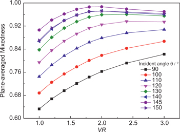
Effect of VR on cross-sectional averaged mixedness at different θ values (Axial position z/D=2, Re_m =3.13×10⁴).

4.4 Effect of Reynolds number

Further study on the effect of gas velocity on mixing is needed because the highest mainstream Reynolds number of experiments we conducted is only 5.64×10⁴, while a Reynolds number of 3.13×10⁵–6.26×10⁵ will be used in the syngas quenching process. The good agreement between experimental and simulation data at both Re_m=3.13×10⁴ and Re_m=5.64×10⁴ allowed us to use simulation to study mixing behavior at higher mainstream Reynolds number. Figure 12 shows the cross-sectional averaged mixedness ηˉ at different axial positions and Re_m of 6.26×10⁴, 1.88×10⁵, 3.13×10⁵ and 6.26×10⁵. Other operating parameters are θ=145° and VR=2. The profiles of ηˉ are similar for the four mainstream Reynolds numbers, indicating that the mixedness only slightly depends on the mainstream Reynolds number at a fixed velocity ratio VR. This is consistent with the works of Smith, Talpallikar, and Holdeman (1991) and Holdeman et al. (1997), who reported that the primary independent flow variables in the mixing of confined circular jets in a straight duct are jet-to-mainstream mass-flow ratio and momentum-flux ratio. At constant momentum-flux ratio, variation in Reynolds number has only a second-order effect on mixing. Since neither of mass-flow ratio nor momentum-flux ratio was changed in our simulations, the change of mixedness distribution should be insignificant.

Figure 12:

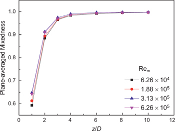
Effect of Re_m on cross-sectional averaged mixedness at different axial positions (VR=2, θ=145°).

It should be pointed out that increasing Reynolds number results in two opposing phenomena: one is the decrease in the residence time of gas in the mixing apparatus, causing a decrease in the mixing time of jets and mainstream; and the other is the increase in turbulent viscosity. Since the mixing process is caused by jet spreading, i. e. the entrainment of surrounding fluid by jets due to turbulent viscosity (Kandakure et al. 2009), the increase of turbulent viscosity leads to more intensive mixing. Those two opposing phenomena counterbalance and the spatial distribution of mixedness is almost independent of the Reynolds number. The independence on the Reynolds number suggests that the results obtained at a relatively low Reynolds number are also valuable for the design of a syngas quenching process operated at a high Reynolds number up to 6.26×10⁵.

References

1. Arora, P., Saha, A.K., 2011. Three-dimensional Numerical Study of Flow and Species Transport in an Elevated Jet in Crossflow. Int. J. Heat Mass Transfer 54, 92–105.10.1016/j.ijheatmasstransfer.2010.07.068Suche in Google Scholar
2. Bachtler, M., Schnur, R.R., Passler, P., Scheidsteger, O., Kastenhuber, W., Schlindwein, G., Konig, R., 1995. Process for the Production of Acetylene and Synthesis Gas. U.S. Patent 5824834.Suche in Google Scholar
3. Ben-Yakar, A., Mungal, M.G., Hanson, R.K., 2006. Time Evolution and Mixing Characteristics of Hydrogen and Ethylene Transverse Jets in Supersonic Crossflows. Phys. Fluids 18, 1131–1151.10.1063/1.2139684Suche in Google Scholar
4. Berg, C.H.O., 1950. Process and Apparatus for Acetylene Production. U.S. Patent 2679540.Suche in Google Scholar
5. Bixler, G.H., Coberly, C.W., 1953. Wulff Process Acetylene. Ind. Eng. Chem. 45, 2596–2606.10.1021/ie50528a018Suche in Google Scholar
6. Chai, X., Iyer, P.S., Mahesh, K., 2015. Numerical Study of High Speed Jets in Crossflow. J. Fluid Mech. 785, 152–188.10.1017/jfm.2015.612Suche in Google Scholar
7. Coletti, F., Benson, M.J., Ling, J., Elkins, C.J., Eaton, J.K., 2013. Turbulent Transport in an Inclined Jet in Crossflow. Int. J. Heat Fluid Flow 43, 149–160.10.1016/j.ijheatfluidflow.2013.06.001Suche in Google Scholar
8. Danckwerts, P.V., 1952. The Definition and Measurement of Some Characteristics of Mixtures. Appl. Sci. Res., Sect. A 3, 279–296.10.1016/B978-0-08-026250-5.50050-2Suche in Google Scholar
9. Earl, G.K., 1982. Calcium Carbide/Water Acetylene Gas Generator. U.S. Patent 4444159.Suche in Google Scholar
10. Elliott, J., McClure, H.H., 1958. Production of Acetylene by the Partial Oxidation of Hydrocarbons. U.S. Patent 2945074.Suche in Google Scholar
11. Erwin, L., Werner, A., Wilhelm, S.F., 1960. Production of Acetylene by Partial Oxidation of Hydrocarbons and Apparatus Therefor. U.S. Patent 2966533.Suche in Google Scholar
12. Esmaeili, M., Afshari, A., Jaberi, F.A., 2015. Turbulent Mixing in Non-Isothermal Jet in Crossflow. Int. J. Heat Mass Transfer 89, 1239–1257.10.1016/j.ijheatmasstransfer.2015.05.055Suche in Google Scholar
13. Fitzgerald, S.D., Holly, E.R., 1981. Jet Injections for Optimum Mixing in Pipe Flow. J. Hydraul. Div., Am. Soc. Civ. Eng. 107, 1179–1195.10.1061/JYCEAJ.0005741Suche in Google Scholar
14. Fluent, 2006. Fluent 6.3 User’s Guide, Fluent Inc., Lebanon, New Hampshire.Suche in Google Scholar
15. Fuller, R.P., Wu, P.K., Nejad, A.S., Schetz, J., 1998. Comparison of Physical and Aerodynamic Ramps as Fuel Injectors in Supersonic Flow. J. Propul. Power 14, 135–145.10.2514/2.5278Suche in Google Scholar
16. Galezzo. F.C.C., Donnert, G., Habisreuther, P., Zarzalis, N., Valdes, R.J., Krebs, W., 2011. Measurement and Simulations of Turbulent Mixing in a Jet in Crossflow. J. Eng. Gas Turbines Power 133, 061504–1.10.1115/GT2010-22709Suche in Google Scholar
17. Giorges, A.T.G., Forney, L.J., Wang, X., 2001. Numerical Study of Multi-jet Mixing. Chem. Eng. Res. Des. 79, 515–522.10.1205/02638760152424280Suche in Google Scholar
18. Gutmark, E.J., Ibrahim, I.M., Murugappan, S., 2008. Circular and Noncircular Subsonic Jets in Cross Flow. Phys. Fluids 20, 075110.10.1063/1.2946444Suche in Google Scholar
19. Gutmark, E.J., Ibrahim, I.M., Murugappan, S., 2011. Dynamics of Single and Twin Circular Jets in Cross Flow. Exp. Fluids 50, 653–663.10.1007/s00348-010-0965-2Suche in Google Scholar
20. Happel, J., Kramer, L., 1967. Acetylene and Hydrogen from the Pyrolysis of Methane. Ind. Eng. Chem. 59, 39–50.10.1021/ie50685a008Suche in Google Scholar
21. Hassan, E., Boles, J., Aono, H., Davis, D., Wei, S., 2013. Supersonic Jet and Crossflow Interaction: Computational Modeling. Prog. Aeronaut. Sci. 57, 1–24.10.1016/j.paerosci.2012.06.002Suche in Google Scholar
22. Holdeman, J.D., 1993. Mixing of Multiple Jets with a Subsonic Crossflow. Prog. Energy Combust. Sci. 19, 31–70.10.1016/0360-1285(93)90021-6Suche in Google Scholar
23. Holdeman, J.D., Liscinsky, D.S., Bain, D.B., 1999. Mixing of Multiple Jets with a Confined Subsonic Crossflow: Part II–Opposed Rows of Orifices in Rectangular Ducts. J. Eng. Gas Turbines Power 121, 551–562.10.1115/97-GT-439Suche in Google Scholar
24. Holdeman, J.D., Liscinsky, D.S., Oechsle, V.L., Samuelsen, G.S., Smith, C.E., 1997. Mixing of Multiple Jets with a Confined Subsonic Crossflow: Part I–Cylindrical Duct. J. Eng. Gas Turbines Power119, 852–862.10.1115/1.2817065Suche in Google Scholar
25. Holmen, A., Olsvik, O., Rokstad, O.A., 1995. Pyrolysis of Natural Gas: Chemistry and Process Concepts. Fuel Process. Technol. 42, 249–267.10.1016/0378-3820(94)00109-7Suche in Google Scholar
26. Hwang, R.R., Chiang, T.P., 1995. Numerical Simulation of Vertical Forced Plume in a Crossflow of Stably Stratified Fluid. J. Fluids Eng. 117, 696–705.10.1115/1.2817325Suche in Google Scholar
27. Issakhanian, E., Elkins, C.J., Eaton, J.K., 2012. In-Hole and Mainflow Velocity Measurements of Low-Momentum Jets in Crossflow Emanating from Short Holes. Exp. Fluids 53, 1765–1778.10.1007/s00348-012-1397-ySuche in Google Scholar
28. Ivanova, E., Noll, B., Aigner, M., Ivanova, E., Noll, B., Aigner, M., 2012. A Numerical Study on the Turbulent Schmidt Numbers in a Jet in Crossflow. ASME Turbo Expo 2012: Turbine Technical Conference and Exposition (Vol. 135, pp. 949–960). American Society of Mechanical Engineers.10.1115/GT2012-69294Suche in Google Scholar
29. Kalifa, R.B., Habli, S., Saïd, N.M., Bournot, H., Palec, G.L., 2014. Numerical and Experimental Study of a Jet in a Crossflow for Different Velocity Ratio. J. Braz. Soc. Mech. Sci. Eng. 36, 743–762.10.1007/s40430-014-0129-zSuche in Google Scholar
30. Kandakure, M.T., Patkar, V.C., Patwardhan, A.W., Patwardhan, J.A., 2009. Mixing with Jets in Cross-flow. Ind. Eng. Chem. Res. 48, 6820–6829.10.1021/ie801863aSuche in Google Scholar
31. Kartaev, E.V., Emel’Kin, V.А., Ktalkherman M.G., Kuz’Min, V.I., Aul’Chenko, S.М., Vashenko, S.P., 2014. Analysis of Mixing of Impinging Radial Jets with Crossflow in the Regime of Counter Flow Jet Formation. Chem. Eng. Sci. 119, 1–9.10.1016/j.ces.2014.07.062Suche in Google Scholar
32. Kartaev, E.V., Emelkin, V.А., Ktalkherman, M.G., Aulchenko, S.М., Vashenko, S.P., Kuzmin, V.I., 2015. Formation of Counter Flow Jet Resulting from Impingement of Multiple Jets Radially Injected in a Crossflow. Exp. Therm. Fluid Sci. 68, 310–321.10.1016/j.expthermflusci.2015.05.009Suche in Google Scholar
33. Karvinen, A., Ahlstedt, H., 2005. Comparison of Turbulence Models in Case of Jet in Crossflow using Commercial CFD Code. Eng. Turbul. Modell. Exp. 6, 399–408.10.1016/B978-008044544-1/50038-8Suche in Google Scholar
34. Kim S.E., Choudhury D., Patel B., 1997. Computations of Complex Turbulent Flows Using the Commercial Code FLUENT. In Proceedings of the ICASE/ LaRC/ AFOSR. Symposium on Modeling Complex Turbulent Flows, Hampton, Virginia.Suche in Google Scholar
35. Kolar, V., Takao, H., Todoroki, T., Savory, E., Okamoto, S., Toy, N., 2003. Vorticity Transport within Twin Jets in Crossflow. Exp. Therm. Fluid Sci. 27, 563–571.10.1016/S0894-1777(02)00270-4Suche in Google Scholar
36. Kroll, J.T., Sowa, W.A., Samuelsen, G.S., 2000. Optimization of Orifice Geometry for Crossflow Mixing in a Cylindrical Duct. J. Propul. Power 16, 929–938.10.2514/2.5669Suche in Google Scholar
37. Ktalkherman, M.G., Emelkin, V.A., Pozdnyakov, B.A., 2010. Influence of the Geometrical and Gasdynamic Parameters of a Mixer on the Mixing of Radial Jets Colliding with a Crossflow. J. Eng. Phys. Thermophys. 83, 539–548.10.1007/s10891-010-0375-6Suche in Google Scholar
38. Ktalkherman, M.G., Namyatov, I.G., 2008. Pyrolysis of Hydrocarbons in a Heat-carrier Flow with Fast Mixing of the Components. Combust. Explos. Shock Waves 44, 529–534.10.1007/s10573-008-0081-2Suche in Google Scholar
39. Launder, B.E., Spalding, D.B., 1972. Lectures in Mathematical Models of Turbulence, Academic Press, London.Suche in Google Scholar
40. Li, Q., (Ph.D. Thesis) 2013. Non-Catalytic Partial Oxidation of Methane to Produce Acetylene and Synthesis Gas, Tsinghua University. (in Chinese)Suche in Google Scholar
41. Li, Z.W., Huai, W.X., Qian, Z.D., 2012. Study on the Flow Field and Concentration Characteristics of the Multiple Tandem Jets in Crossflow. Sci. China Technol Sci. 55, 2778–2788.10.1007/s11431-012-4964-9Suche in Google Scholar
42. Liu, Y., Wang, T., Li, Q., Wang, D., 2011. A study of Acetylene Production by Methane Flaming in a Partial oxidation Reactor. Chin. J. Chem. Eng. 19, 424–433.10.1016/S1004-9541(11)60002-5Suche in Google Scholar
43. Mahesh, K., 2013. The Interaction of Jets with Crossflow. Annu. Rev. Fluid Mech. 45, 379–407.10.1146/annurev-fluid-120710-101115Suche in Google Scholar
44. Muppidi, S., Mahesh, K., 2008. Direct Numerical Simulation of Passive Scalar Transport in Transverse Jets. J. Fluid Mech. 598, 335–6010.1017/S0022112007000055Suche in Google Scholar
45. Naik-Nimbalkar, V.S., Suryawanshi, A.D., Patwardhan, A.W., Banerjee, I., Padmakumar, G., Vaidyanathan, G., 2011. Twin Jets in Cross-flow. Chem. Eng. Sci. 66, 2616–2626.10.1016/j.ces.2011.03.018Suche in Google Scholar
46. Russ, M., Grossschmidt, D., Renze, P., Vicari, M., Neuhauser, H., Ehrhardt, K.R., Weichert, C., 2013. Process and Apparatus for Preparing Acetylene and Synthesis Gas. U.S. Patent 8506924.Suche in Google Scholar
47. Russell, J.G., 1958. Oil Quench Process for Partial Oxidation of Hydrocarbon gases. U.S. Patent 3022148.Suche in Google Scholar
48. Samokhin, A.V., Alekseev, N.V., Kornev, S.A., Sinaiskii, M.A., Blagoveschenskiy, Y.V., Kolesnikov, A.V., 2013. Tungsten Carbide and Vanadium Carbide Nanopowders Synthesis in DC Plasma Reactor. Plasma Chem. Plasma Process 33, 605–61610.1007/s11090-013-9445-9Suche in Google Scholar
49. Santiago, J.G., Dutton, J.C., 1997. Velocity Measurements of a Jet Injected into a Supersonic Crossflow. J. Propul. Power 13, 264–273.10.2514/2.5158Suche in Google Scholar
50. Shih T.H., Liou W.W., Shabbir A., Yang Z., Zhu J., 1995. A New k-ε Eddy-Viscosity Model for High Reynolds Number Turbulent Flows – Model Development and Validation. Comput. Fluids 24, 227–238.10.1016/0045-7930(94)00032-TSuche in Google Scholar
51. Smith, C.E., Talpallikar, M.V., Holdeman, J.D., 1991. A CFD Study of Jet Mixing in Reduced Flow Areas for Lower Combustor Emissions. AIAA Pap. 90–2460.10.2514/6.1991-2460Suche in Google Scholar
52. Stapf, D., Passler, P., Bachtler, M., Scheidsteger, O., Bartenbach, B., 2002. Preparation of Acetylene and Synthesis gas. U.S. Patent 6365792.Suche in Google Scholar
53. Sundararaj, S., Selladurai, V., 2013. Flow and Mixing Pattern of Transverse Turbulent Jet in Venturi-Jet Mixer. Arabian J. Sci. Eng. 38, 3563–3573.10.1007/s13369-013-0643-9Suche in Google Scholar
54. Urson, H., Lightstone, M.F., Thomson, M.J., 2001. A Numerical Study of Jets in a Reacting Crossflow. Numer. Heat Transfer Part A 40, 689–714.10.1080/104077801753289800Suche in Google Scholar
55. Vranos, A., Liscinsky, D.S., True, B., Holdeman J.D., 1991. Experimental Study of Cross-Stream Mixing in a Cylindrical Duct. In AIAA, SAE, ASME, and ASEE, 27th Joint Propulsion Conference.10.2514/6.1991-2459Suche in Google Scholar
56. Wang, T., Li, Q., Wang, D., 2012. Method and device for quenching and heat recovery in partial oxidation process of natural gas. CN Patent CN102329189A. (in Chinese)Suche in Google Scholar
57. Wang, Z., Zheng, D., 2008. Energy Analysis and Retrofitting of Natural Gas-based Acetylene Process. Chin. J. Chem. Eng. 16, 812–818.10.1016/S1004-9541(08)60161-5Suche in Google Scholar
58. Wilcox, D.C., 1993. Turbulence Modeling for CFD, DCW Industries Inc., La Canada, California.Suche in Google Scholar
59. Willi, D., Otto, F., Erich, K., Ferdinand, M., Walter, T., 1966. Production of Acetylene. U.S. Patent 3242225.Suche in Google Scholar
60. Yao, S., Suzuki, E., Meng, N., Nakayama, A., 2001. A High-efficiency Reactor for the Pulsed Plasma Conversion of Methane. Plasma Chem. Plasma Process. 22, 225–237.10.1023/A:1014843425384Suche in Google Scholar
©2017 by De Gruyter
Artikel in diesem Heft
- Bubble Trajectory in a Bubble Column Reactor using Combined Image Processing and Artificial Neural Network
- Non-linear Radiation Effects in Mixed Convection Stagnation Point Flow along a Vertically Stretching Surface