POD-Galerkin Model for Incompressible Single-Phase Flow in Porous Media

Yi Wang; Bo Yu; Shuyu Sun

doi:10.1515/phys-2016-0061

Article Open Access

POD-Galerkin Model for Incompressible Single-Phase Flow in Porous Media

Yi Wang , Bo Yu and Shuyu Sun

Published/Copyright: December 30, 2016

Published by

Become an author with De Gruyter Brill

Submit Manuscript Author Information Explore this Subject

From the journal Open Physics Volume 14 Issue 1

Abstract

Fast prediction modeling via proper orthogonal decomposition method combined with Galerkin projection is applied to incompressible single-phase fluid flow in porous media. Cases for different configurations of porous media, boundary conditions and problem scales are designed to examine the fidelity and robustness of the model. High precision (relative deviation 1.0 × 10⁻⁴% ~ 2.3 × 10⁻¹%) and large acceleration (speed-up 880 ~ 98454 times) of POD model are found in these cases. Moreover, the computational time of POD model is quite insensitive to the complexity of problems. These results indicate POD model is especially suitable for large-scale complex problems in engineering.

Keywords: POD; Porous Media; Single-Phase Flow; Model Reduction

PACS: 47.56.+r

1 Introduction

Fluid flow in porous media is a very important physical phenomenon in many aspects of engineering, such as catalytic reaction in chemical engineering [1], transport of oil/gas/water in petroleum engineering [2], etc. Numerical simulation is needed to predict the flow details [3]. This usually leads to numerous simulations and long-time iterations of a large-partial-differential-equation system per simulation [4–9]. Therefore, the total computational time is usually very long and as a result this type of simulation is not practical for the demands of fast prediction in engineering.

Proper orthogonal decomposition (POD) is an efficient method for reducing the computational time through Galerkin projection with good precision [10]. It has been successfully used in wide range of physics and engineering problems, such as turbulent flow [11, 12], heat transfer [13, 14], oil transportation [15], etc. Thus, the utilization of POD-Galerkin method can be expected to greatly increase the efficiency of simulation in porous media. Although POD method for flow in subsurface porous media was discussed in reference, emphasis was mainly on precision [16–18] rather than acceleration. In this paper, we demonstrate high acceleration and precision of POD-Galerkin model for incompressible single-phase flow in porous media via a series of numerical cases. For statement convenience, we only discuss two-dimensional cases here.

2 Establishment of the POD-Galerkin Model

2.1 Description of the Original Governing Equations

Incompressible single-phase flow in porous media are described by the mass balance equation (Eq. (1)) and the Darcy’s law (Eq. (2)) as follows:

(1)∇⋅u=q

(2)u=−kμ∇p−ρg∇z

where u=ui→+vj→ is Darcy velocity, k=kxxkyy is permeability tensor, p is pressure, g is the gravitational acceleration, q is injection or production rate, ρ and µ are density and dynamic viscosity of fluid respectively, z is the depth. The components of Darcy velocity and permeability are u, k_xx in the x direction and v, k_yy in the y direction. Gravitational acceleration can be included into the piezometric head (Φ = p -ρgz) so that the treatment is the same as that without gravity. It is neglected here for convenience. Substituting Eq. (2) without gravity to Eq. (1), we can obtain:

(3)−∇⋅kμ∇p=q

Eq. (3) shows that computational time is primarily used in the computation of pressure, usually requiring long-time iterations for large systems. POD-Galerkin model is a good choice for greatly reducing the computational time of Eq. (3). The main procedure to establish the model will be stated below.

2.2 POD-Galerkin Model

POD method is data dependent so that the first step is collection of samples through computation of governing equations (Eq. (2) and Eq. (3)). Finite difference method (FDM) is used here to obtain discrete equations of the governing equations, which are solved via the Gauss-Seidel iteration method combined with the successive over relaxation method. The samples can be expressed as follows:

(4)S1=p11p21⋮pL1,S2=p12p22⋮pL2,S3=p13p23⋮pL3,…,SN=p1Np2N⋮pLN

where S₁, S₂, S₃, · · · , S_N represent the serials of samples, N is the number of samples, L is the number of grid points (including boundary). All the samples compose an L × N sample matrix:

(5)S=S1,S2,S3,⋯,SN

The number of grid points is usually much larger than the number of samples, i.e. L>>N. Thus, the snapshot POD [19, 20] should be used to obtain POD modes:

(6)ϕn=1σnSVn

where ϕ_n are referred to the POD modes (n = 1~ N), σ_n and V_n are the singular values and eigenvectors obtained from singular value decomposition (SVD) of matrix S^TS.

With the known singular values, we can define:

(7)en=σn/∑i=1Mσi×100%,En=∑j=1nσj/∑i=1Mσi×100%

where e_n is the energy contribution of the nth POD mode to the whole energy spectrum of POD, E_n is the cumulative energy contribution of the first n POD modes (ϕ₁ ~ ϕ_n) to the whole energy spectrum. The higher energy contributions indicate more features of samples captured by POD modes so as to more importance of these modes. This property will be used to determine the selection of POD modes in Section 3.

With the known modes ϕ_n, pressure can be reconstructed by the linear combination:

(8)p=∑n=1Mcnϕn

where M(≤ N) is the number of used POD modes, c_n are unknown coefficients, independent of space, to be calculated from the POD model. To derive this model, we substitute Eq. (8) to Eq. (3) and obtain:

(9)−∑n=1Mcn∂∂xkxxμ∂ϕn∂x+∂∂ykyyμ∂ϕn∂y=q

Project Eq. (9) onto the POD mode ϕ_m (m = 1~ M):

(10)−∑n=1Mcn∫0ly∫0lx∂∂xkxxμ∂ϕn∂x+∂∂ykyyμ∂ϕn∂yϕmdxdy=∫0ly∫0lxqϕmdxdy

Simplify Eq. (10) via the integration by part:

(11)−Δy∑j=1nyϕmkxxμ∂p∂xnx+1,j−ϕmkxxμ∂p∂x0,j+Δx∑i=1nxϕmkyyμ∂p∂yi,ny+1−ϕmkyyμ∂p∂yi,0−ΔxΔy∑n=1Mcn∑j=1ny∑i=1nxkxxμ∂ϕn∂x∂ϕm∂x+kyyμ∂ϕn∂y∂ϕm∂yi,j=ΔxΔy∑j=1ny∑i=1nxqϕmi,j

The undefined symbols in Eqs. (10) and (11) are illustrated in Fig. 1. Uniform mesh and staggered grid method are utilized with grid number of 100 × 100 and domain size of 100 m × 100 m in this paper.

Figure 1

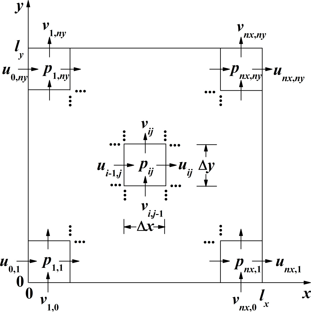
Domain and staggered grid

For a Dirichlet boundary condition (known boundary pressure), any one of the following equations could be used:

(12)∂p∂x0,j=∑n=1Mcnϕn1,j−p0,jΔx/2,∂p∂xnx+1,j=pnx+1,j−∑n=1Mcnϕnnx,jΔx/2,∂p∂yi,0=∑n=1Mcnϕni,1−pi,0Δy/2,∂p∂yi,ny+1=pi,ny+1−∑n=1Mcnϕni,nyΔy/2

For a Neumann boundary condition (known boundary velocity), any one of the following equations could be used:

(13)−kxxμ∂p∂x0,j=u0,j,−kxxμ∂p∂xnx+1,j=unx,j,−kyyμ∂p∂yi,0=vi,0,−kyyμ∂p∂yi,ny+1=vi,ny

Combining the Dirichlet and Neumann boundary conditions in Eq. (11), the final expression for POD-Galerkin model is:

(14)∑n=1MAm,ncn=bm

where

Am,n=∑j=1ny∑i=1nxkxxμ∂ϕn∂x∂ϕm∂x+kyyμ∂ϕn∂y∂ϕm∂yi,j+2Δx2∑j=1nyDirixnx+1,jϕnnx,jϕmkxxμnx+1,j+Dirix0,jϕn1,jϕmkxxμ0,j+2Δy2∑i=1nxDiriyi,ny+1ϕni,nyϕmkyyμi,ny+1+Diriyi,0ϕni,1ϕmkyyμi,0bm=∑j=1ny∑i=1nxqϕmi,j+2Δx2∑j=1nyDirixnx+1,jϕmkxxμnx+1,jpnx+1,j+Dirix0,jϕmkxxμ0,jp0,j+2Δy2∑i=1nxDiriyi,ny+1ϕmkyyμi,ny+1pi,ny+1+Diriyi,0ϕmkyyμi,0pi,0−1Δx∑j=1ny1−Dirixnx+1,j⋅ϕmnx+1,junx,j−1−Dirix0,jϕm0,ju0,j−1Δy∑i=1nx1−Diriyi,ny+1ϕmi,ny+1vi,ny−1−Diriyi,0ϕmi,0vi,0

Dirix and Diriy are 1 for Dirichlet boundaries and 0 for Neumann boundaries.

For a prediction case that is different from samples, the coefficients can be calculated from Eq. (14) so that the pressure under the prediction condition can be calculated directly from Eq. (14) instead of Eq. (3). From the above derivation, we know the dimension of Eq. (14) is much smaller than that of Eq. (3), i.e. M ≤ N ≪ L. Thus, computational time can be reduced largely via POD-Galerkin model.

3 Results and Discussion

In this section, the POD-Galerkin model obtained in Section 2 is applied to incompressible single-phase flow in different types of porous media to examine the precision and acceleration abilities of the model. Precision is measured by the relative deviation:

(15)ε=pPOD−pFDM/pFDM×100%

Acceleration is measured by the ratio:

(16)r=tFDM/tPOD

where p_FDM and p_POD are the pressure fields calculated from Eq. (3) via FDM and Eq. (14) & (8) via POD. t_FDM and t_POD are corresponding CPU time. ||·|| represents the L₁-norm.

3.1 A Homogeneous Isotropic Porous Medium

Firstly, a homogeneous isotropic porous medium is considered. Permeability components are the same over the whole domain with the value of 100 md (1 md = 9.869233 × 10⁻¹⁶ m²). The parameters and boundary conditions are shown in Fig. 2. Each boundary pressure takes two different values: p₁ = {50, 60} mH₂O, p₂ = {20, 40} mH₂O (1 mH₂O = 9800 Pa). Thus, the number of the samples is 2 × 2 = 4.

Figure 2

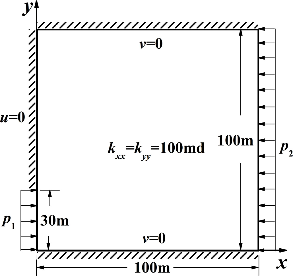
A homogeneous isotropic porous medium

According to Section 2, the maximum number of POD modes is equivalent to the number of samples, i.e. four in this case. The selection of the mode number depends on the actual precision of sample reconstruction. The precisions using different number of POD modes are shown in Table. 1. It is obvious that the optimal number of POD modes is two with the relative deviation as low as 0%~ 2 × 10⁻⁴%. The inclusion of ϕ₃ and ϕ₄ generates very large deviations. The reason is analyzed in Fig. 3 and Table. 2. In Fig. 3, the smooth distributions of modes ϕ₁ and ϕ₂ refect the sample distribution correctly (Fig. 3(a) & 3(b)) while the fluctuated distributions of modes ϕ₃ and ϕ₄ indicate the unphysical numerical errors because flows in porous media are low-speed laminar flow without fluctuations. This is further verified in Table. 2 that ϕ₃ and ϕ₄ do not contain any energy indicating that they do not contain any information about the samples. These two modes are only numerical errors produced by the SVD. The sole inclusion of ϕ₁ could not generate accurate enough reconstructed results (e = 2.82% ~ 10.11% in Table. 1) although its energy contribution is very high (e_n = 99.35%). The inclusion of ϕ₂ supplements a small energy contribution (e_n = 0.65%) to make the POD model capture the whole important information (E_n = 100%) and promote model precision largely (e = 0% ~ 2 × 10⁻⁴% in Table. 1). Thus, ϕ₂ cannot be neglected even if its energy contribution is quite lower than ϕ₁. The same situations also occur in Sections 3.2 ~ 3.5 according to the computational results so that the discussion on the selection of POD modes will not be repeated in the following sections and ϕ₁ and ϕ₂ will be used directly.

Figure 3

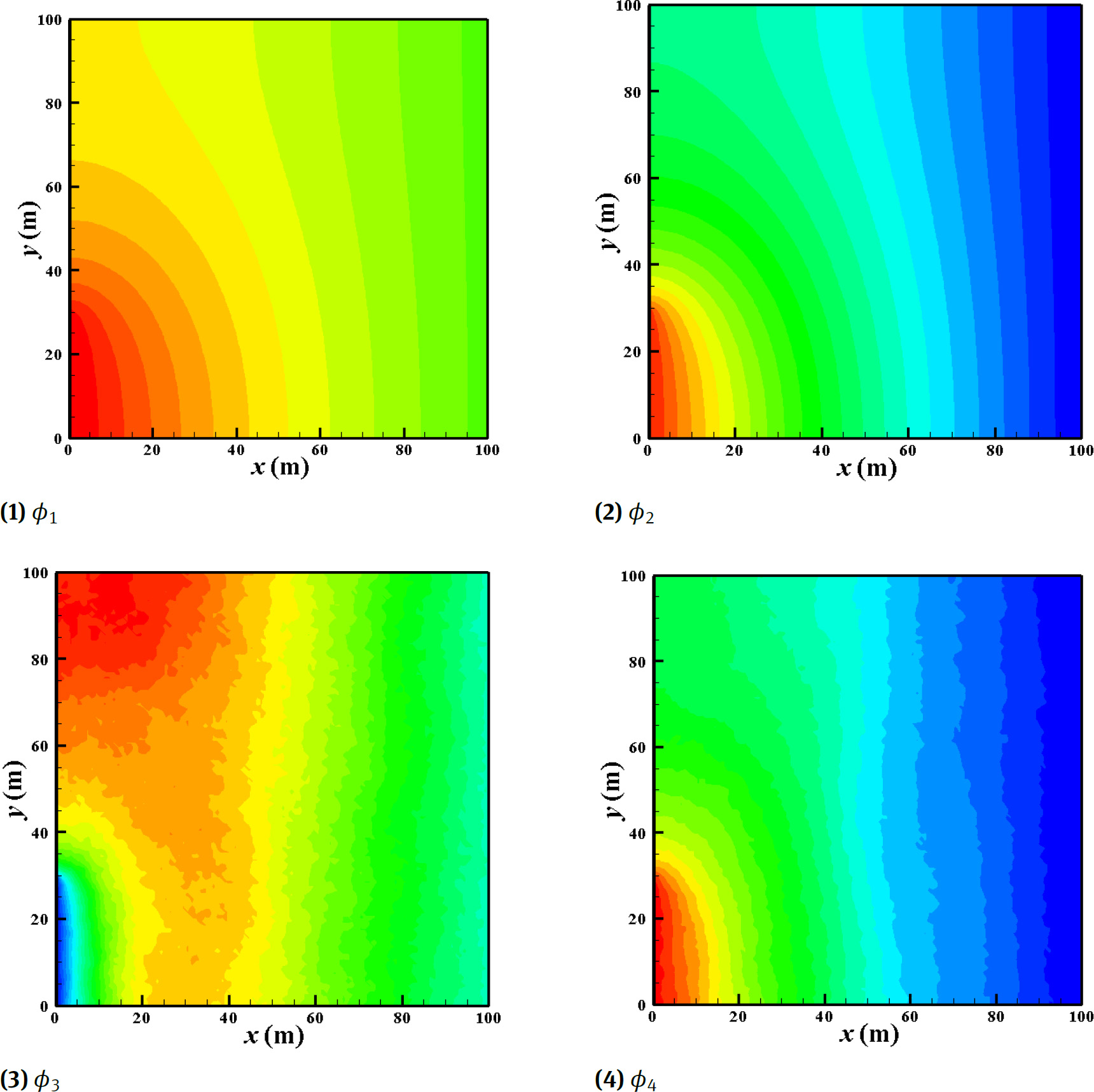
Distribution of POD modes

Table 1

Relative deviation of sample reconstruction

M	S₁	S₂	S₃	S₄
1	6.75%	6.13%	10.11%	2.82%
2	2 × 10⁻⁴%	0%	2 ×10⁻⁴%	1 × 10⁻⁴%
3	84.35%	70.00%	88.09%	73.69%
4	84.36%	70.04%	88.09%	73.72%

Table 2

Energy contribution of the POD modes

n	1	2	3	4
e_n	99.35%	0.65%	0%	0%
E_n	99.35%	100%	100%	100%

To validate the precision of POD model for predicting cases different from the samples, prediction conditions are designed as p₁ = {10, 20, 30, 40, 50, 60, 70, 80, 90, 100} mH₂O, p₂ = {5, 15, 25, 35, 45, 55, 65, 75, 85, 95} mH₂O so that the number of prediction cases is 10 × 10 = 100. The relative deviations of 100 cases are shown in Fig. 4 with the maximum value of 4.0 × 10⁻⁴% and the minimum value of 0%, indicating good performance of solutions globally. Three typical cases (a, b, c) are selected to show the local solutions of the flow field. The comparisons are shown in Fig. 5. Local solutions of p, u, v using POD coincide very well with those using FDM, no matter whether the boundary conditions fall within (a) or out of (b, c) the sample scope. Even if the boundary condition of case c (p₁ < p₂) is opposite to that of samples (p₁ > p₂), the deviation is also small enough. Therefore, the POD model is proved to be very accurate for the homogeneous isotropic porous medium.

Figure 4

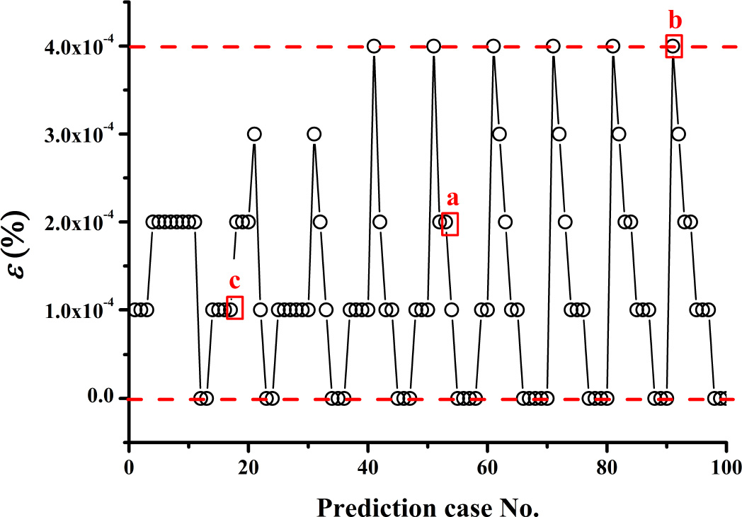
Relative deviation of the prediction cases for a homogeneous isotropic porous medium

Figure 5

Comparison of flow fields for 3 typical prediction cases for a homogeneous isotropic porous medium: from left to right are p, u, v respectively; black solid line-FDM, red dotted line-POD

To validate the computational speed of the POD model, computational time is compared in Table. 3. The computational time of the training stage (both the 4 sample cases and the SVD) only costs once for the POD model. Once the training stage is completed, we can use the POD model to predict any number of cases without further sampling and decomposition. Thus, the one-time cost of training time should not be considered into the acceleration ratio of POD model, even if it is small. For the 100 prediction cases, the computational times of FDM and POD are 678 s and 0.2s respectively. The acceleration ratio is high (3390), indicating excellent acceleration ability of POD model.

Table 3

Computational time comparison for a homogeneous isotropic porous medium

Training	Sampling Time (4 cases)	27s	One-time
Stage	Decomposition Time	3.6s	cost
Prediction	FDM (100 cases)	678s	r = 678/
Stage	POD (100 cases)	0.2s	0.2 = 3390

3.2 A Homogeneous Anisotropic Porous Medium

In this section, a homogeneous anisotropic porous medium is considered as shown in Fig. 6. The permeability tensor is unique all over the domain, but the component k_xx is 100 times larger than component k_yy. Different boundary conditions are adopted to avoid particularity. Four sample cases are taken with the same boundary pressures of Section 3.1. The 100 prediction cases are designed with the boundary pressures:

Figure 6

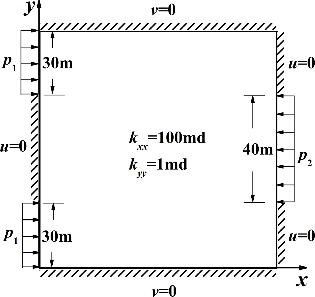
A homogeneous anisotropic porous medium

p₁ = {10, 20, 30, 40, 50, 60, 70, 80, 90, 100} mH₂O,

p₂ = {15, 25, 35, 45, 55, 65, 75, 85, 95, 105} mH₂O.

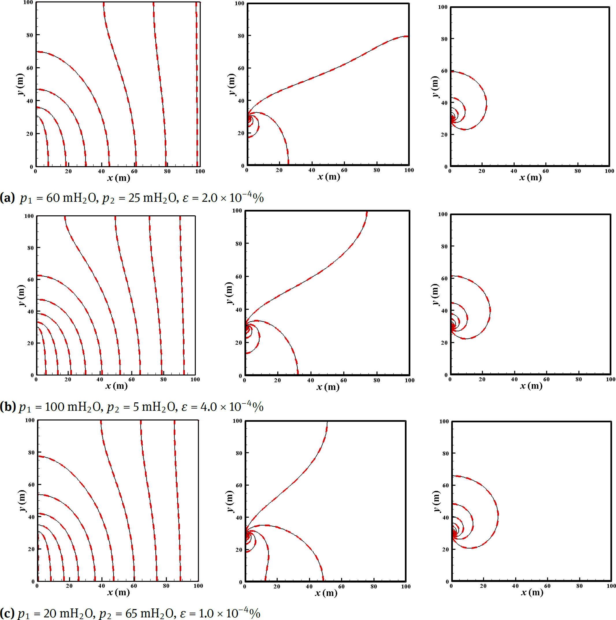
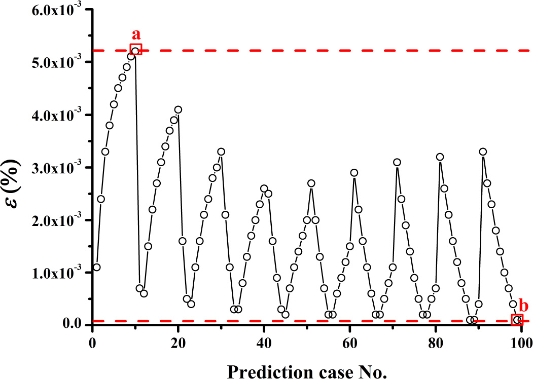
Fig. 7 shows the high precision of POD model for 100 cases. The relative deviations are low (1.0 × 10⁻⁴% ~ 5.2 × 10⁻³%). The precision is further examined using two cases (a, b) with the maximum and minimum deviations. For these cases, POD results agree very well with FDM results (as shown in Fig. 8). Thus, POD model is very accurate for homogeneous anisotropic porous medium.

Figure 7

Relative deviation of the prediction cases for a homogeneous anisotropic porous medium

Figure 8

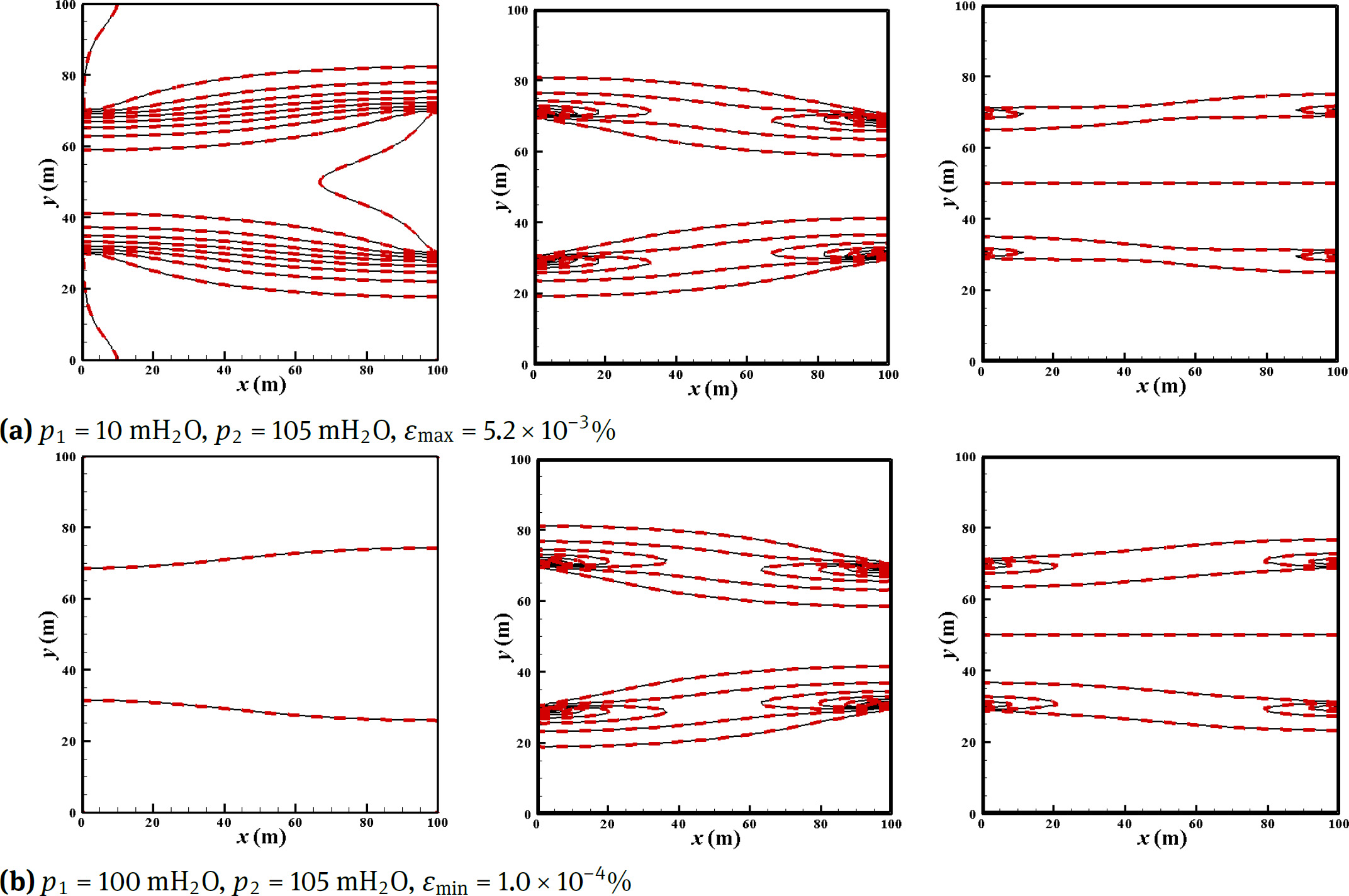
Comparison of flow fields for 2 typical prediction cases for a homogeneous anisotropic porous medium: from left to right are p, u, v respectively; black solid line-FDM, red dotted line-POD

For the 100 prediction cases, the computational times are compared in Table. 4 for FDM and POD. The acceleration ratio is still very high (r = 2300), showing the good acceleration ability of the POD model.

Table 4

Computational time comparison for a homogeneous anisotropic porous medium

Training	Sampling Time (4 cases)	26s	One-time
Stage	Decomposition Time	0.2s	cost
Prediction	FDM (100 cases)	621s	r = 621/
Stage	POD (100 cases)	0.27s	0.27 = 2300

3.3 An Inhomogeneous Isotropic Porous Medium

In this section, an inhomogeneous isotropic porous medium is designed as shown in Fig. 9. The distribution of permeability is not uniform with a small value in the “H”-shape zone and a large value in other zone, but the two components k_xx and k_yy are always equal to each other. Sample cases are designed as p₁ = {50, 55} mH₂O, p₂ = {60, 65} mH₂O. Prediction cases are designed as p₁ = {0, 10, 20, 30, 40, 50, 60, 70, 80, 90} mH₂O, p₂ = {10, 20, 30, 40, 50, 60, 70, 80, 90, 100} mH₂O. It should be noticed that there are no flows for the 9 cases when p₁ = p₂ so those are not discussed here. Therefore, the total effective prediction cases must be 10 × 10 - 9 = 91.

Figure 9

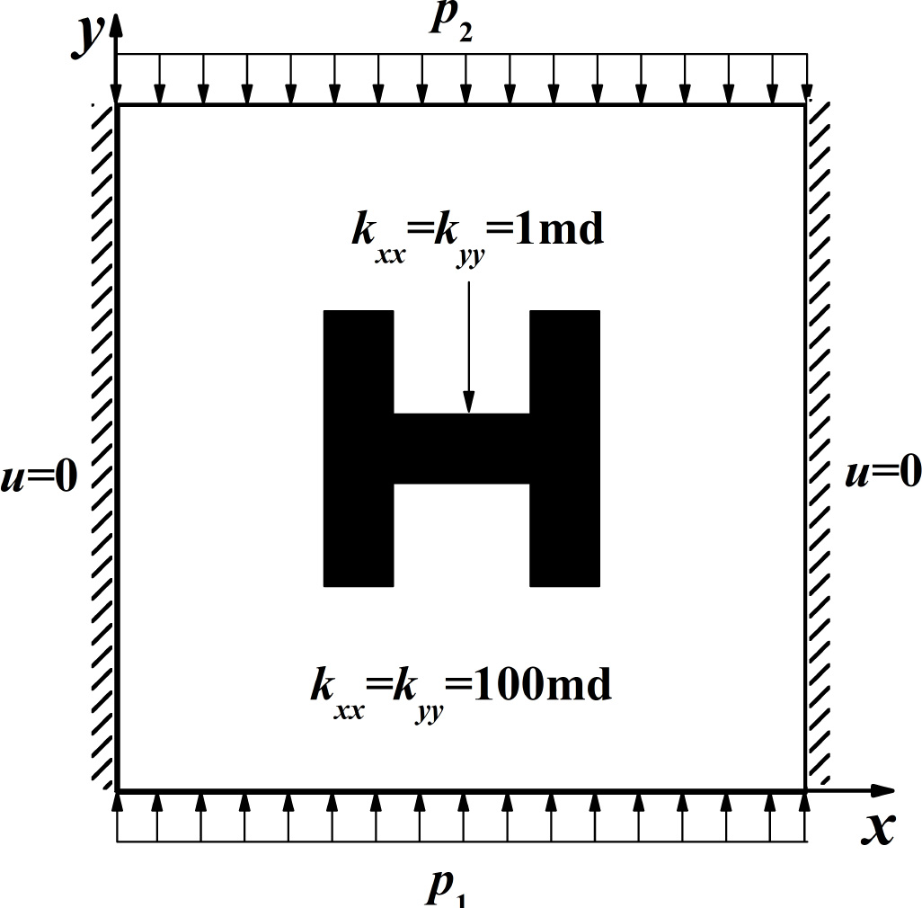
An inhomogeneous isotropic porous medium

With the 2 POD modes extracted from the 4 samples, predictions for 91 cases are made. The relative deviations are very low (7.0 × 10⁻⁴%~ 1.4 × 10⁻²%) as shown in Fig. 10. Pressure and velocity coincide very well with each other for both POD and FDM in the two cases with the maximum and minimum deviations (Fig. 11). Thus, POD model is again proven to be very accurate for inhomogeneous isotropic porous medium.

Figure 10

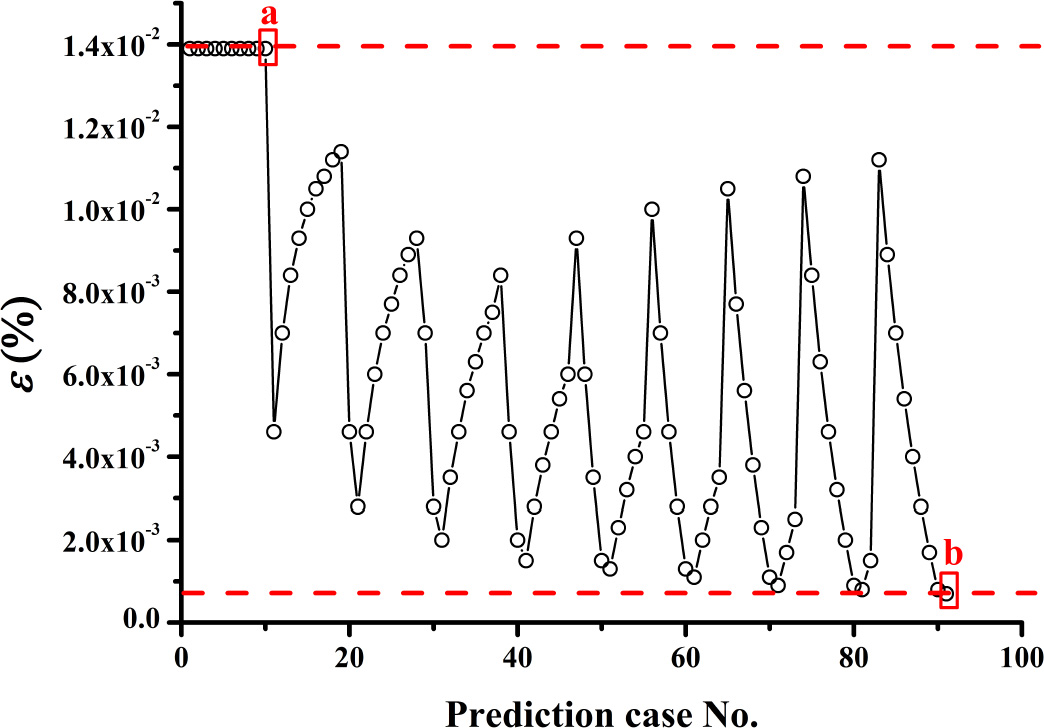
Relative deviation of the prediction cases for an inhomogeneous isotropic porous medium

Figure 11

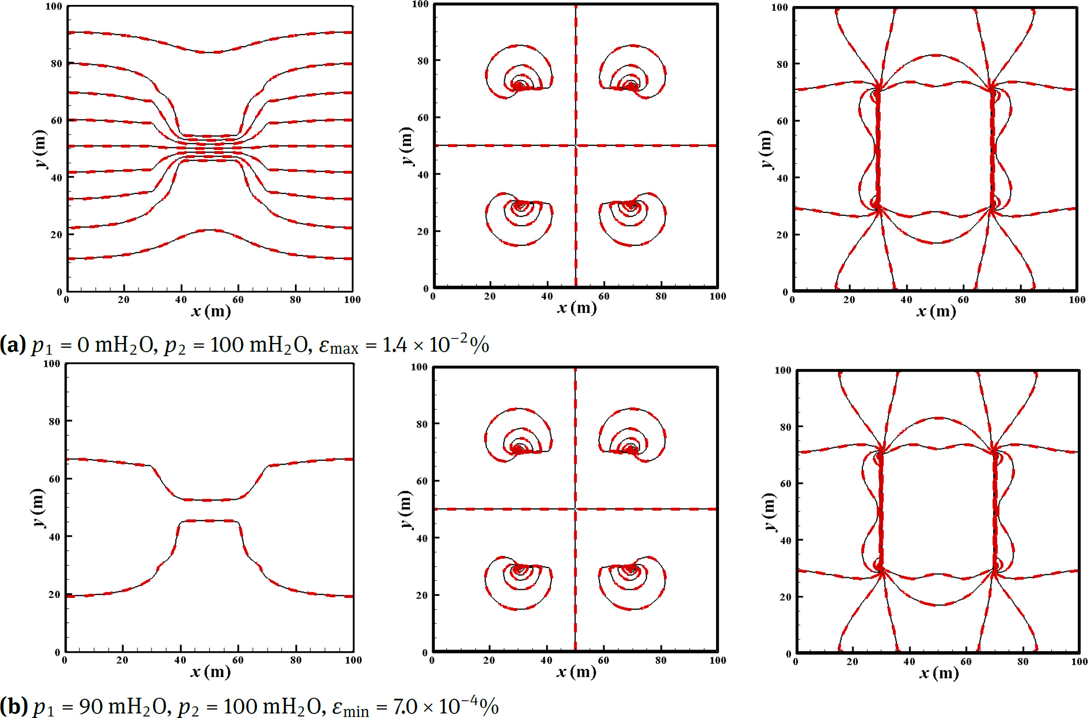
Comparison of flow fields for 2 typical prediction cases for an inhomogeneous isotropic porous medium: from left to right are p, u, v respectively; black solid line-FDM, red dotted line-POD

Table. 5 shows the acceleration ratio of the POD model decreases to 880. The decrease is due to the shorter computational time for FDM caused by different permeability field and boundary conditions. Nevertheless, the acceleration ratio is still attractive.

Table 5

Computational time comparison for an inhomogeneous isotropic porous medium

Training	Sampling Time (4 cases)	12s	One-time
Stage	Decomposition Time	3.2s	cost
Prediction	FDM (91 cases)	264s	r = 264/
Stage	POD (91 cases)	0.3s	0.3 = 880

3.4 An Inhomogeneous Anisotropic Porous Medium

To examine the POD model in a more complex case, we let k_xx > k_yy in the “H”-shape zone and k_xx < k_yy in the other zone so that an inhomogeneous anisotropic porous medium is designed as shown in Fig. 12. All other sampling and prediction conditions are the same as Section 3.3.

Figure 12

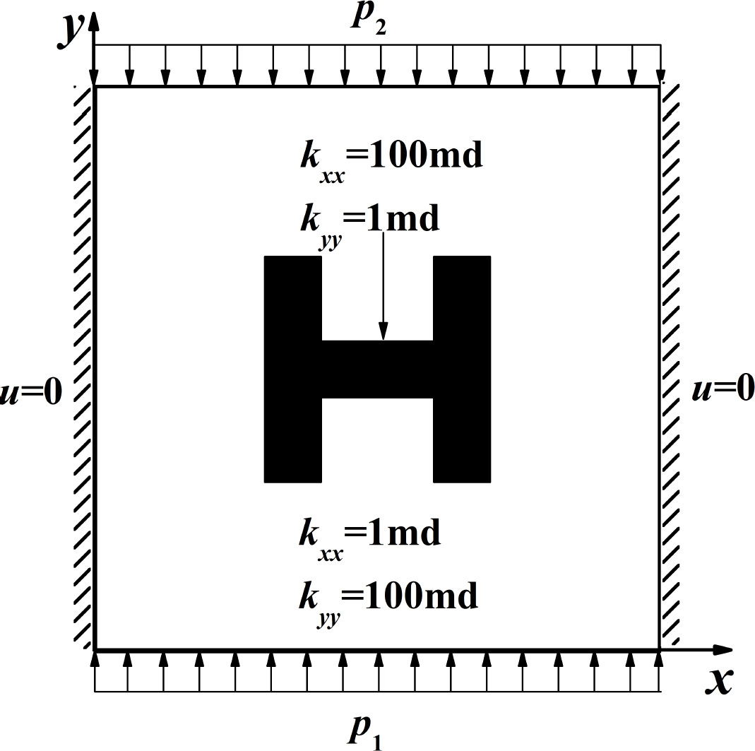
An inhomogeneous anisotropic porous medium

Figure 13

Relative deviation of the prediction cases for an inhomogeneous anisotropic porous medium

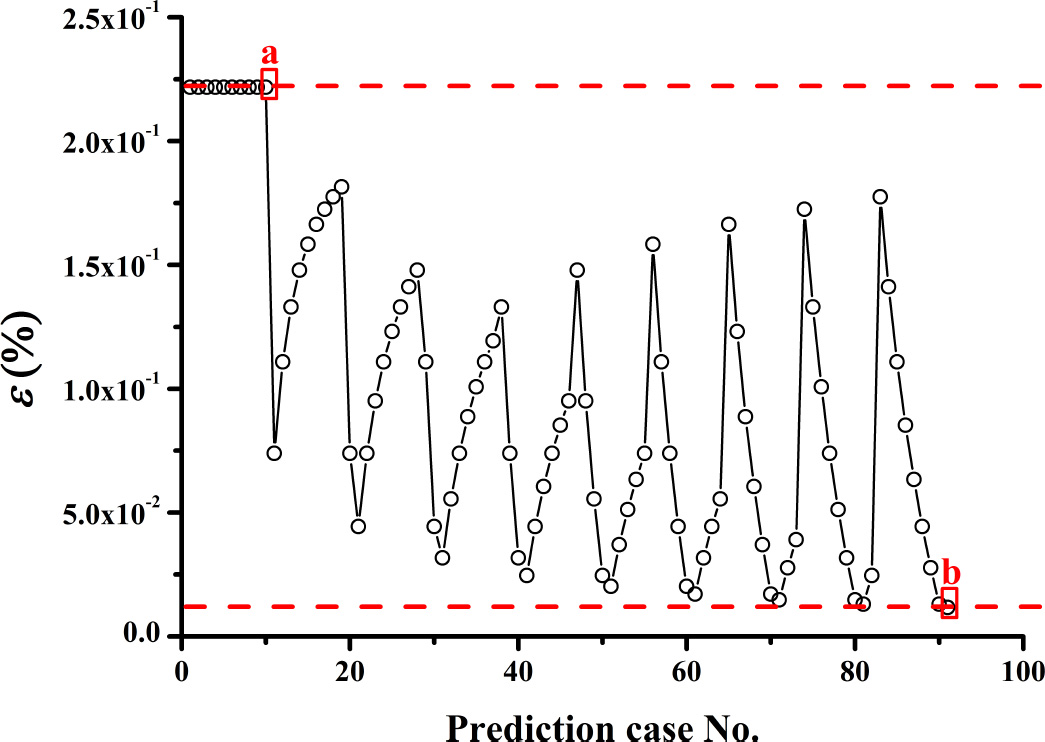
The relative deviations of the prediction cases are apparently larger than the previous situations, indicating that the precision of POD model may decrease along with the increasing complexity of the problems. However, the precision is still high (ɛ = 1.2 × 10⁻²% ~ 2.2 × 10⁻¹%) in Fig. 13. The flow fields still coincide with each other very well for both POD and FDM results, in the two cases with maximum and minimum deviations (Fig. 14). Thus, the POD model has also proven to be very accurate for inhomogeneous isotropic porous medium.

Figure 14

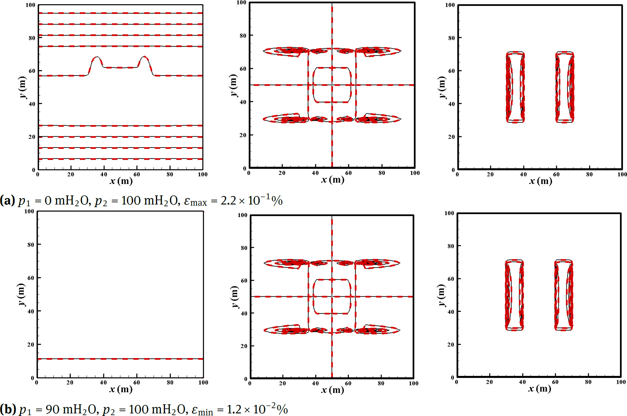
Comparison of flow fields for 2 typical prediction cases for an inhomogeneous anisotropic porous medium: from left to right are p, u, v respectively; black solid line-FDM, red dotted line-POD

Figure 15

A random porous medium

Table. 6 shows the acceleration ratio of the prediction cases. It is 98454, which exceeds all other cases in the above sections. The extremely high acceleration ratio is due to longer computational time for FDM due to much higher complexity of the problem.

Table 6

Computational time comparison for an inhomogeneous anisotropic porous medium

Training	Sampling Time (4 cases)	543s One-time
Stage	Decomposition Time	0.14s cost
Prediction	FDM (91 cases)	12799s r = 12799/
Stage	POD (91 cases)	0.13s 0.13 = 98454

3.5 A Random Porous Medium

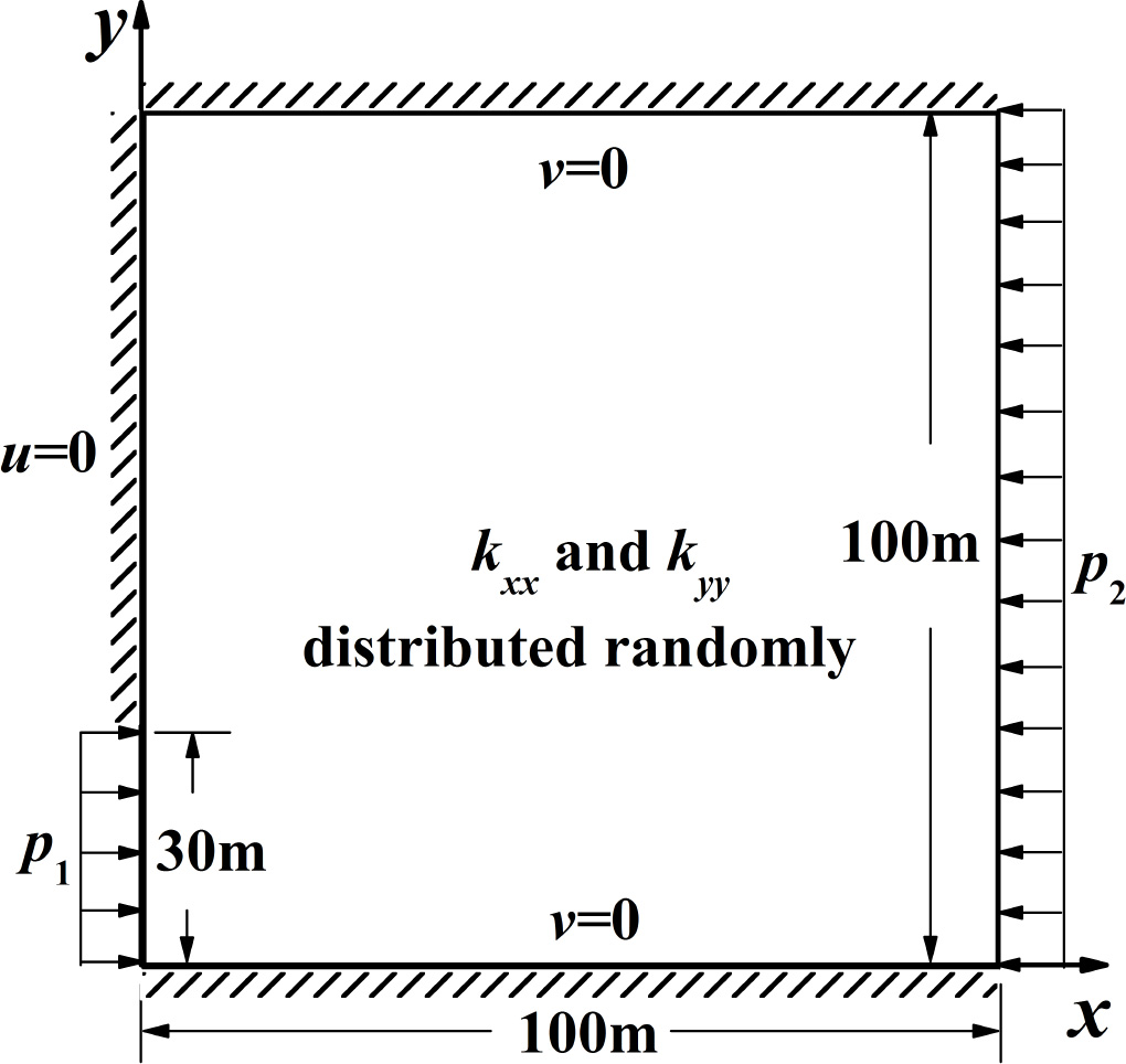
From the comparisons in Sections 3.1 ~ 3.4, we confirmed that POD model has high fidelity in precision and large acceleration in computational time for either homogeneous or inhomogeneous and either isotropic or anisotropic porous media. However, the computational settings are basically ideal, e.g. the “H”-shaped permeability distribution. Permeability fields in real engineering are more complex than these structures. In order to achieve stronger conclusions, we use randomly distributed, inhomogeneous and anisotropic permeability field and recall other settings in the case in Section 3.1. The domain and parameters are shown in Fig. 15 while the permeability fields are shown in Fig. 16.Two components of permeability are even in different ranges: k_xx for 1 md ~ 10 md and k_yy for 10 md ~ 100 md. The sampling conditions are: p₁ = {30, 60} mH₂O, p₂ = {20, 80} mH₂O. The prediction conditions are:

p₁ = {10, 20, 30, 40, 50, 60, 70, 80, 90, 100, 110} mH₂O,

p₂ = (0, 15, 30, 45, 60, 75, 90, 105, 120, 135) mH₂O.

Table 7

Computational time comparison for a random porous medium

Training	Sampling Time (4 cases)	109s	One-time
Stage	Decomposition Time	0.2s	cost
Prediction	FDM (107 cases)	3266s	r = 3266/
Stage	POD (107 cases)	0.23s	0.23 = 14200

Figure 16

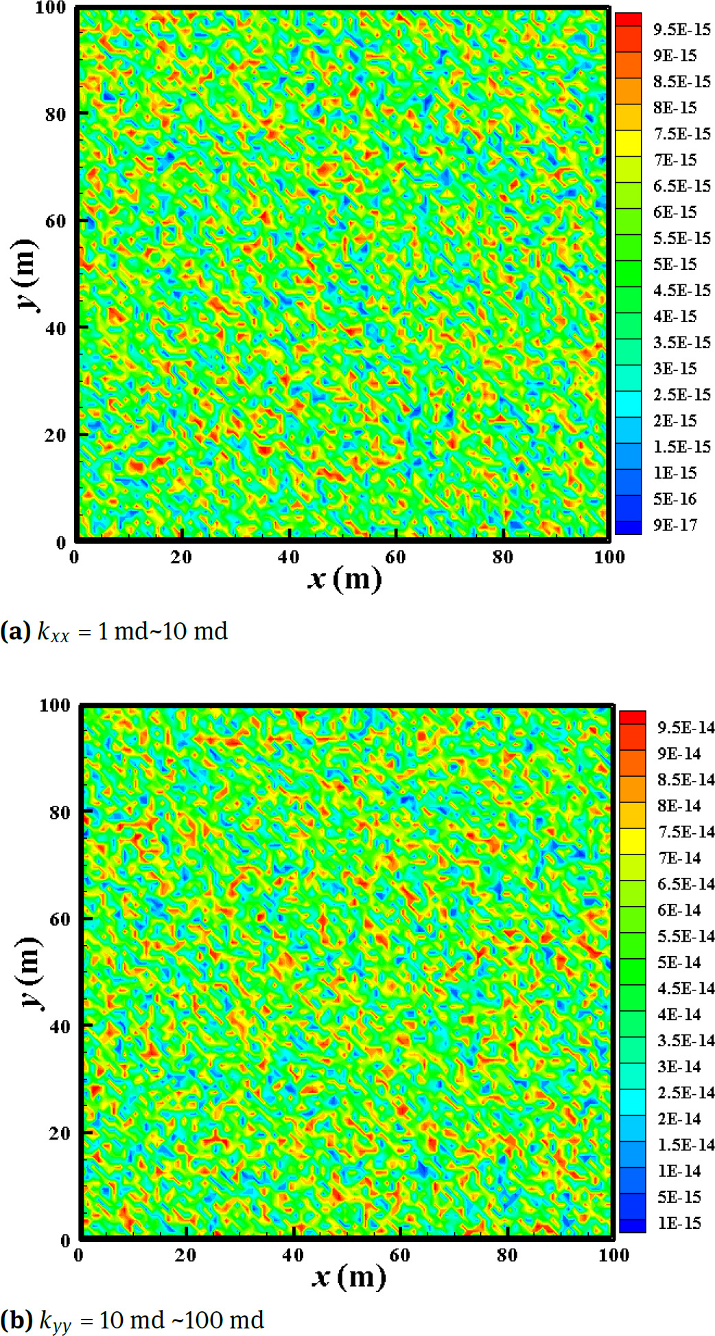
Random distribution of the inhomogeneous-anisotropic permeability field

As shown in Fig. 17, the relative deviations are 4.5 × 10⁻³% ~ 2.3 × 10⁻¹% even if 107 prediction cases are predicted by only 2 POD modes for the random permeability field. This overall precision is high enough to be accepted in engineering. To identify local precision, 4 typical cases (a, b, c, d) among these 107 cases are selected to compare the pressure field and the velocity field obtained by POD and FDM. If the same style of the previous comparison (e.g. style in Fig. 5, Fig. 8, Fig. 11, Fig. 14) is adopted, the local details cannot be recognized clearly. Therefore, we change to a new comparison style in Fig. 18, where the figures on the first row represent results by FDM while the figures on the second row represent the results by POD. The comparison shows that POD results agree very well with the FDM results, even though the prediction conditions of the 4 cases are quite different from the sampling conditions. Acceleration ratio on the computational time is also surprisingly high (r = 14200).

Figure 17

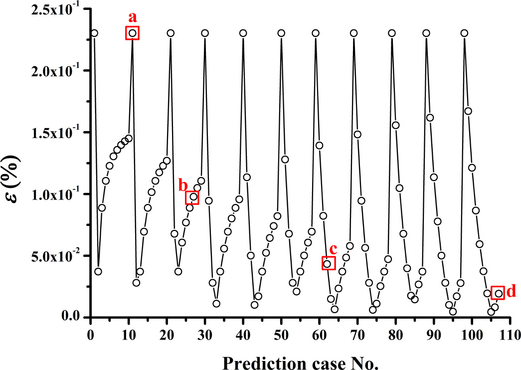
Relative deviation of the prediction cases for a random porous medium

Figure 18

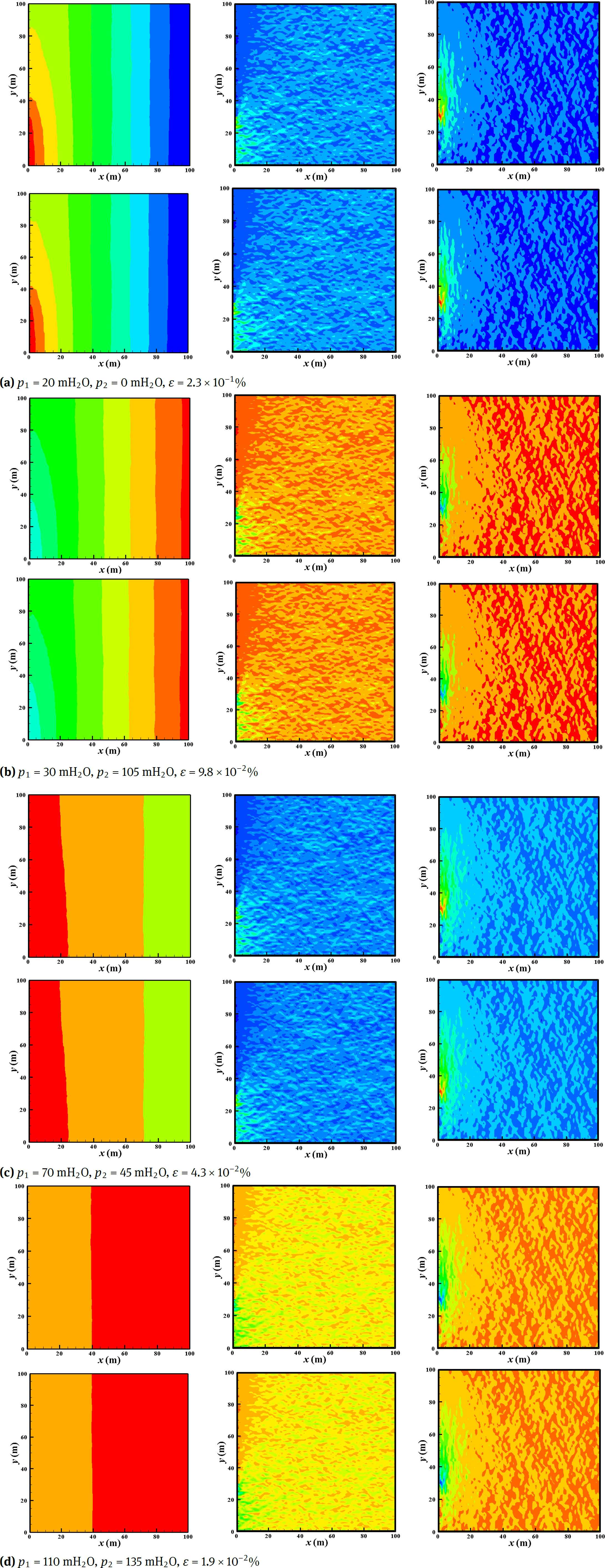
Comparison of flow fields for 4 typical prediction cases for a random porous medium: from left to right are p, u, v respectively; first row-FDM, second row-POD

4 Conclusion

POD-Galerkin modeling method is successfully applied to incompressible single-phase flow in porous media. Precision and acceleration of the model are discussed under different permeability and boundary settings. Our primary conclusions are as follows:

The acceleration ratio is very large with very high precision for fluid flows in different types of porous media (r = 880~ 98454 and ɛ = 1.0 × 10⁻⁴% ~ 2.3 × 10⁻¹%).
The computational time of FDM is very sensitive to complexity of problems such as configuration of permeability, the number of prediction cases, boundary conditions, etc. It is usually higher for more complex porous media (264 s ~ 12799 s). However, the computational time of POD is quite insensitive to the complexity of problems. It is only in a very narrow range (0.13 s ~ 0.3 s) for cases with configuration of permeability, the number of prediction cases and boundary condition quite different from each other. The reason for this phenomenon is that complexity strongly affects the iteration process of large equation systems in FDM (Eq. (3)) but the effects of complexity on much smaller equation systems in POD (Eq. (14)) is very weak.
According to (1) and (2), the POD-Galerkin model has potential to satisfy the demands of fast prediction in engineering where complex porous media are usually encountered.

Acknowledgement

The work presented in this paper has been supported by National Natural Science Foundation of China (NSFC) (No.51576210, No.51476073, No.51325603), Science Foundation of China University of Petroleum-Beijing (No.2462015BJB03, No.2462015YQ0409, No. C201602) and also supported in part by funding from King Abdullah University of Science and Technology (KAUST) through the grant BAS/1/1351-01-01.

References

[1] Li X., Chen J., Xu M., Huai X., Xin F., Cai J., Lattice Boltzmann simulation of catalytic reaction in porous media with buoyancy, Appl. Therm. Eng., 2014, 70, 586-592.10.1016/j.applthermaleng.2014.04.034Search in Google Scholar

[2] Salehi-Shabestari A., Ahmadpour A., Raisee M., Sadeghy K., Flow and displacement of waxy crude oils in a homogenous porous medium: a numerical study, J. Non-Newton. Fluid Mech., 2016, 235, 47-63.10.1016/j.jnnfm.2016.07.005Search in Google Scholar

[3] Chen J., Chen Z., Three-dimensional superconvergent gradient recoveryon tetrahedral meshes, Int.J.Numer. Meth. Eng., 2016, 10.1002/nme.5229.Search in Google Scholar

[4] Moortgat J., Sun S., Firoozabadi A., Compositional modeling of three-phase flow with gravity using higher-order finite element methods, Water Resour. Res., 2011, 47, W05511.10.1029/2010WR009801Search in Google Scholar

[5] Sun S., Liu J., A locally conservative finite element method based on piecewise constant enrichment of the continuous Galerkin method, SIAM J. Sci. Comput., 2009, 31(4), 2528-2548.10.1137/080722953Search in Google Scholar

[6] Sun S., Wheeler M.F., Analysis of discontinuous Galerkin methods for multicomponent reactive transport problems, Comput. Math. Appl., 2006, 52(5), 637-650.10.1016/j.camwa.2006.10.004Search in Google Scholar

[7] Sun S., Wheeler M.F., A dynamic, adaptive, locally conservative and nonconforming solution strategy for transport phenomena in chemical engineering, Chem. Eng. Commun., 2006, 193(12), 1527-1545.10.1080/00986440600584284Search in Google Scholar

[8] Sun S., Wheeler M.F., Discontinuous Galerkin methods for simulating bioreactive transport of viruses in porous media, Adv. Water Resour., 2007, 30(6-7), 1696-1710.10.1016/j.advwatres.2006.05.033Search in Google Scholar

[9] Wang Y., Sun S., Direct calculation of permeability by high-accurate finite difference and numerical integration methods, Commun. Comput. Phys., 2016, 20(2), 405-440.10.4208/cicp.210815.240316aSearch in Google Scholar

[10] Bergmann M., Bruneau C.H., Iollo A., Enablers for robust POD models, J. Comput. Phys., 2009, 228 (2), 516-538.10.1016/j.jcp.2008.09.024Search in Google Scholar

[11] Wang Y., Yu B., Wu X., Wang P., POD and wavelet analyses on the flow structures of a polymer drag-reducing flow based on DNS data, Int. J. Heat Mass Transf., 2012, 55(17-18), 4849-4861.10.1016/j.ijheatmasstransfer.2012.04.055Search in Google Scholar

[12] Podvin B.,A proper-orthogonal-decomposition-based model for the wall layer of a turbulent channel flow, Phys. Fluids, 2009, 21(1), 94-100.10.1063/1.3068759Search in Google Scholar

[13] Wang Y., Yu B., Cao Z., Zou W., Yu G., A comparative study of POD interpolation and POD projection methods for fast and accurate prediction of heat transfer problems, Int. J. Heat Mass Transf., 2012, 55(17-18), 4827-4836.10.1016/j.ijheatmasstransfer.2012.04.053Search in Google Scholar

[14] Wang Y., Yu B., Sun S., Fast prediction method for steady-state heat convection, Chem. Eng. Technol., 2012, 35(4): 668-678.10.1002/ceat.201100428Search in Google Scholar

[15] Han D., Yu B., Wang Y., Zhao Y„ Yu G., Fast thermal simulation of a heated crude oil pipeline with a BFC-based POD reduced-order model, Appl. Therm. Eng., 2015, 88, 217-229.10.1016/j.applthermaleng.2014.10.017Search in Google Scholar

[16] Ghommem M., Calo V.M., Efendiev Y., Mode decomposition methods for flows in high-contrast porous media. A global approach, J. Comput. Phys., 2014, 257, 400-413.10.1016/j.jcp.2013.09.031Search in Google Scholar

[17] Ghommem M., Presho M., Calo V.M., Efendiev Y., Mode decomposition methods for flows in high-contrast porous media. Global-local approach, J. Comput. Phys., 2013, 253, 226-238.10.1016/j.jcp.2013.06.033Search in Google Scholar

[18] Efendiev Y. Galvis J., Gildin E., Local-global multiscale model reduction for flows in high-contrast heterogeneous media, J. Comput. Phys., 2012, 231, 8100-8113.10.1016/j.jcp.2012.07.032Search in Google Scholar

[19] Sirovich L., Kirby M., Low-dimensional procedure for the characterization of human faces, J. Opt. Soc. Am. A-Opt. Image Sci. Vis., 1987, 4(3), 529-524.10.1364/JOSAA.4.000519Search in Google Scholar

[20] Sirovich L., Turbulent and dynamics of coherent structure: I-III, Q. Appl. Math., 1987, 45, 561-590.10.1090/qam/910462Search in Google Scholar

Received: 2016-8-29

Accepted: 2016-10-21

Published Online: 2016-12-30

Published in Print: 2016-1-1

This work is licensed under the Creative Commons Attribution-NonCommercial-NoDerivatives 3.0 License.