Exact solutions of the Biswas-Milovic equation, the ZK(m,n,k) equation and the K(m,n) equation using the generalized Kudryashov method
-
EL Sayed M.E. Zayed
 and
Abdul-Ghani Al-Nowehy
and
Abdul-Ghani Al-Nowehy

Abstract
In this article, we apply the generalized Kudryashov method for finding exact solutions of three nonlinear partial differential equations (PDEs), namely: the Biswas-Milovic equation with dual-power law nonlinearity; the Zakharov--Kuznetsov equation (ZK(m,n,k)); and the K(m,n) equation with the generalized evolution term. As a result, many analytical exact solutions are obtained including symmetrical Fibonacci function solutions, and hyperbolic function solutions. Physical explanations for certain solutions of the three nonlinear PDEs are obtained.
1 Introduction
The research area of nonlinear partial differential equations (PDEs) has been very active for the past few decades. There are many types of nonlinear PDEs that appear in various areas of the physical and mathematical sciences. Much effort has been expended on constructing exact solutions to these nonlinear PDEs, motivated by their important role in the study of nonlinear physical phenomena. Nonlinear phenomena appears in various scientific and engineering fields, such as fluid mechanics, plasma physics, optical fibers, biology, solid state physics, chemical kinematics, chemical physics, and geo-chemistry. In recent years, a number of powerful and efficient methods for finding analytic solutions to nonlinear equations have drawn a lot of interest by a diverse group of scientists. These include, for example: Hirota’s bilinear transformation method [1, 2]; the tanh-function method [3, 4]; the (G′/G)-expansion method [5–10]; the Exp-function method [11–14]; the multiple exp-function method [15–17]; the symmetry method [18, 19]; the modified simple equation method [20–22]; the improved (G′/G)-expansion method [23]; a multiple extended trial equation method [24]; the Jacobi elliptic function expansion method [25, 26]; the Bäcklund transform method [27, 28]; the generalized Riccati equation method [29]; the modified extended Fan sub equation method [30]; the auxiliary equation method [31, 32]; the first integral method [33, 34]; the modified Kudryashov method [35–42], and the soliton ansatz method [43–70].
The objective of this paper is to apply the generalized Kudryashov method [42] to find the exact solutions of the Biswas-Milovic equation with dual-power law nonlinearity [71, 72], the ZK(m,n,k) [73, 74], and the K(m,n) equation with the generalized evolution term [75].
This paper is organized as follows: in Sec. 2, the description of the generalized Kudryashov method is given. In Sec. 3, we use this method to solve the three aforementioned nonlinear PDEs. In Sec. 4, physical explanations of certain results are presented, and conclusions are discussed in Sec. 5.
2. Description of the generalized Kudryashov method
Starting with a nonlinear PDE in the following form:
where u = u(x, t) is an unknown function, F is a polynomial in u = u (x, t) and its partial derivatives, in which the highest order derivatives and nonlinear terms are involved.
The main steps of the generalized Kudryashov method are described as follows:
Step 1. First, we use the wave transformation:
where k and λ are arbitrary constants with k, λ ≠ 0, in order to reduce equation (2.1) into a nonlinear ordinary differential equation (ODE) with respect to the variable ζ of the form
where H is a polynomial in U(ζ) and its total derivatives U′, U″, U‴, ... such that
Step 2. We assume that the formal solution of the ODE (2.3) can be written in the following rational form:
where 
Taking into consideration (2.4), we obtain
and that similar solutions apply for higher order differentiation terms.
Step 3. Under the terms of the given method, we suppose that the solution of Eq. (2.3) can be written in the following form:
To calculate the values m and n in (2.9), i.e. the pole order for the general solution of Eq. (2.3), we progress as per the classical Kudryashov method by balancing the highest order nonlinear terms and the highest order derivatives of U() in Eq. (2.3). This allows us to derive a formula for m and n and determine their values.
Step 4. We substitute (2.4) into Eq. (2.3) to get a polynomial R (Q) of Q and equate all the coefficients of Qi, (i = 0, 1, 2, ...) to zero, to yield a system of algebraic equations for ai (i = 0, 1, ..., n) and bj (j = 0, 1, ..., m).
Step 5. We solve the algebraic equations obtained in Step 4 using Mathematica or Maple, to get k , and the coefficients of ai (i = 0, 1, ..., n) and bj (j = 0, 1, ..., m). In this way, we attain the exact solutions to Eq. (2.3).
The obtained solutions depended on the symmetrical hyperbolic Fibonacci functions given in [76]. The symmetrical Fibonacci sine, cosine, tangent, and cotangent functions are, respectively, defined as:
3. Applications
In this section we construct the exact solutions in terms of the symmetrical hyperbolic Fibonacci functions of the following three nonlinear PDEs using the generalized Kudryashov method described in Sec. 2:
3.1 Example 1. The Biswas-Milovic equation with dual-power law nonlinearity
In this subsection, we study the Biswas-Milovic equation with dual-power law nonlinearity [71, 72]
where a, b and k are constants, while m, n are positive integers.
If m = 1, then Eq. (3.1.1) becomes the nonlinear Schrödinger equation (NLSE) with dual-power law nonlinearity. In Eq. (3.1.1), the first term is the temporal evolution, while a is the coefficient of group-velocity dispersion (GVD), while b and k are the coefficients of the nonlinear terms. Let us now solve Eq. (3.1.1) using the method of Sec. 2. To this end, we use the wave transformation
where λ, w, μ and v are constants.
Substituting (3.1.2) into (3.1.1), we obtain the nonlinear ODE:
From Eq. (3.1.3) , we deduce that
and
Balancing (Um)″ and U4n + m in (3.1.5), then the following relation is attained:
Then we take into consideration the transformation
Substituting (3.1.7) into equation (3.1.5) we have the new equation
Balancing the vv″ and v4 in (3.1.8), then the following relation is obtained:
If we choose M = 1 and N = 2, then the formal solution of Eq. (3.1.8) has the form:
and consequently
Substituting (3.1.10), (3.1.11) and (3.1.12) into (3.1.8), collecting the coefficients of each power of Qi, (i = 0, 1, ..., 8) and setting each of the coefficients to zero, we obtain the following system of algebraic equations:
Solving the system of algebraic equations (3.1.13) by Maple or Mathematica, we obtain the following sets:
Set 1:
Substituting (3.1.14) into (3.1.10), we get the following solution:
From (3.1.7) and (3.1.15) we have
With the help of (2.10) and (2.11) the exact solution of Eq. (3.1.1) has the form:
or
where
set 2:
Substituting (3.1.21) into (3.1.10), we get the following solution:
From (3.1.7) and (3.1.122) we have
With the help of (2.10) and (2.11) the exact solution of Eq. (3.1.1) has the form:
or
where
set 3:
Consequently,we have the exact solutions of Eq. (3.1.1) in the form:
or
where
On comparing our result (3.1.24), with the result (18) obtained in [71], we conclude that the two results are equivalent with λ = −κ, while our results (3.1.18), (3.1.20), (3.1.25), (3.1.27) and (3.1.28) are new, and not discussed elsewhere.
3.2 Example 2. The Zakharov–Kuznetsov equation (ZK(m,n,k))
In this subsection, we apply the given method to solve the ZK(m,n,k) [73, 74]
where u = u (x, y, t) is a readily differentiable function, λ0, λ1 and λ2 are arbitrary constants while m, n and k are positive integers. The function governs the behaviour of weakly nonlinear ion acoustic waves in a plasma comprising cold ions and hot isothermal electrons in the presence of a uniform magnetic field [77]. Recently, Ma et al. [73] used the auxiliary equation method to find the solutions of the ZK(2,1,1) equation with
This work is concerned with two cases of Eq. (3.2.1):
3.2.1 Case 1: ZK(2,1,1)
In this case Eq. (3.2.1) becomes the form:
To seek travelling wave solutions, we use the wave transformation
where β and γ are arbitrary constants with β, γ ≠ 0, to reduce equation (3.2.2) to the ODE:
Integrating Eq. (3.2.4) with respect to ζ, with zero constant of integration, we get
Balancing the U˶ and U2 in (3.2.5), then we have N = M + 2. If we choose M = 1 and N = 3, then the formal solution of Eq. (3.2.5) has the form:
and consequently,
Substituting (3.2.6) and (3.2.8) into (3.2.5), and equating all the coefficients of Qi, (i = 0, 1, ..., 7) to zero, we get a system of algebraic equations, which can be solved using the Maple, to get the following sets:
Set 1:
Substituting (3.2.9) into (3.1.10), we get the following solution of Eq. (3.2.6):
With the help of (2.10) and (2.11) the exact solution of Eq. (3.2.2) in the form:
where
set 2:
Consequently, we have the exact solutions of Eq. (3.2.2) in the form:
where
If we choose
3.2.2 Case 2: ZK(m,1,1), m ⩾ 3
In this case Eq. (3.2.1) becomes the form:
Using the same wave transformation (3.2.3), to reduce equation (3.2.16) to the ODE:
Integrating Eq. (3.2.17) with respect to ζ, with zero constant of integration, we get
By balancing U″ with Um we have
Substituting (3.2.19) into equation (3.2.18) we have the new equation
Balancing the vv″ and v4 in (3.2.21), then we have N = M + 1. If we choose M = 1 and N = 2, then Eq. (3.2.20) has the same formal solution (3.1.10).
Substituting (3.1.10),(3.1.11) and (3.1.12) into (3.2.20), and equating all the coefficients of Qi,(i = 0, 1, ..., 8) to zero, we get a system of algebraic equations, which can be solved using the aid of Maple or Mathematica, to get the following result:
provided that
Substituting (3.2.21) into (3.1.10), we get the following solution of Eq. (3.2.20):
From (3.2.22) and (3.2.19) we have
With the help of (2.10) and (2.11) the exact solution of Eq. (3.2.16) in the form:
where
3.3 Example 3. The K(m,n) equation
The K(m,n) equation with the generalized evolution term [75, 78, 79] is given by
where, the first term is the generalized evolution term, the second term represents the nonlinearity, and the third term is the dispersion. Also, a , b ∈ R and are constants, while l, m and n ∈ Z+.
Eq. (3.3.1) is the generalized form of the KdV equation, where, in particular, the case l = m = n = 1 leads to the KdV equation. Eq. (3.3.1) appeared for the first time in [78] for l = 1. Thus, Eq. (3.3.1) reduces to the K(m,n) equation for l = 1. Therefore, for l = 1, K(1,1) is the KdV equation while K(2,1) is the mKdV equation. Eq. (3.3.1) has been discussed in [75] using the (G′/G)-expansion method and its exact solutions have been found.
In order to solve Eq. (3.3.1) using the method of section 2, we introduce the wave transformation
where µ and c are constants, to reduce Eq. (3.3.1) to the ODE:
Integrating Eq. (3.3.3) with respect to ζ, with zero constant of integration, we have
Let l = n, balancing (Un)′ and Um+1 in (3.3.4) yields
to reduce Eq. (3.3.4) into the ODE
Balancing the vv″ and v3 in (3.3.6), then we have N = M + 2. If we choose M = 1 and N = 3, then Eq. (3.3.6) has the same formal solution (3.2.6).
Substituting (3.2.6),(3.2.7) and (3.2.8) into (3.3.6), and equating all the coefficients of Qi,(i = 0, 1, ..., 10) to zero, we get a system of algebraic equations, which can be solved using the aid of Maple or Mathematica, to get the following result:
provided that bc>0.
Substituting (3.3.7) into (3.2.6), we get the following solution of Eq. (3.3.6):
From (3.2.8) and (3.2.5) we have
With the help of (2.10) and (2.11) the exact solution of Eq. (3.3.1) in the form:
or
where
4 Physical explanations for some of our solutions
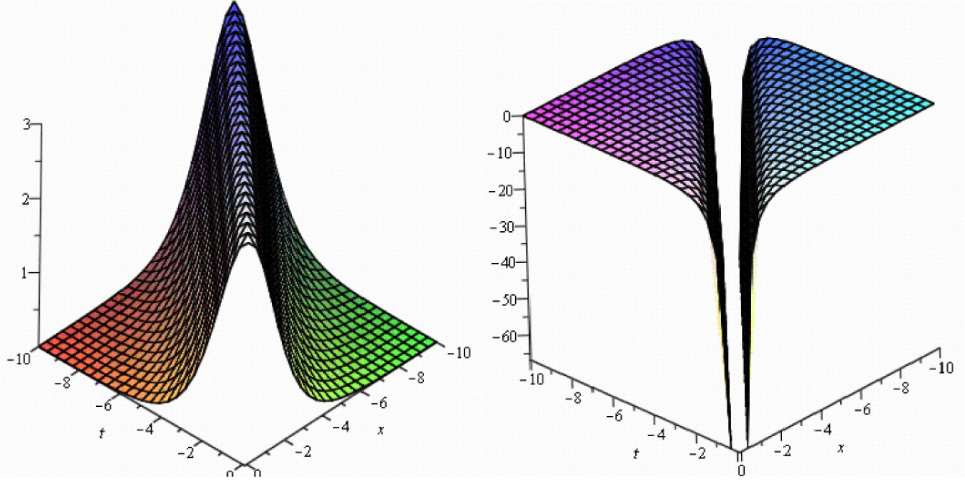
In this section, we will illustrate the application of the results established above. Exact solutions of the results describe different nonlinear waves. The established exact solutions with symmetrical hyperbolic Fibonacci functions are special kinds of solitary waves.
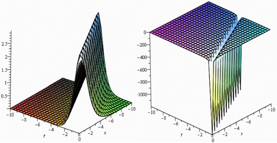
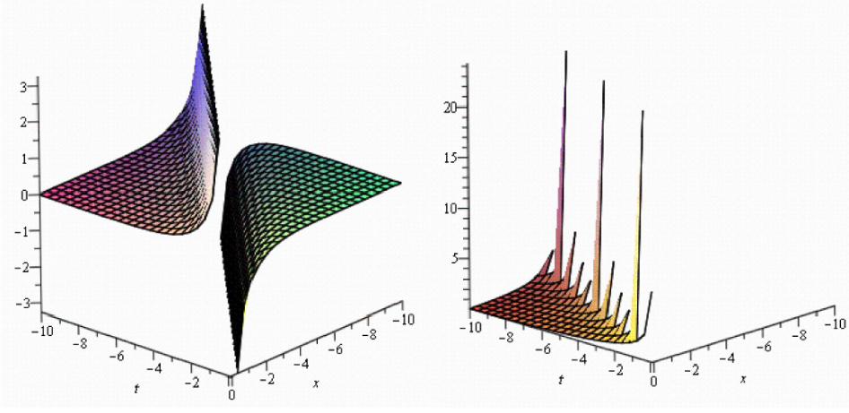
We now examine Figures (1–4) which illustrate a selection of the results obtained above. Specific parameter values are selected, for example: in some of the solutions (3.1.24) and (3.1.25) of the Biswas-Milovic equation with dual-power law nonlinearity with −10 < x, t < 10, solutions (3.2.11) and (3.2.12) of the ZK(2,1,1) with −10 < x, t < 10, solution (3.2.24) of the ZK(m,1,1) with −10 < x, t < 10, solutions (3.3.10) and (3.3.11) of the K(m,n) equation with the generalized evolution with −10 < x, t < 10.
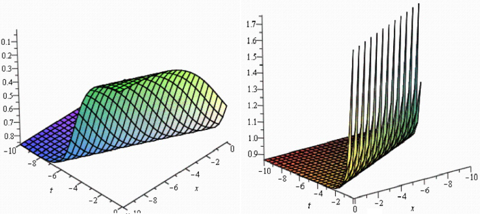
Symmetrical Fibonacci hyperbolic function solutions of the Biswas-Milovic equation with dual-power law nonlinearity when a = b = λ = n = m = 1, K = −1.
Symmetrical Fibonacci hyperbolic function solutions of the ZK(2,1,1) when λ0 = λ1 = λ2 = β = 1, a = e, y = 0.
Symmetrical Fibonacci hyperbolic function solutions of the ZK(m,1,1) when λ0 = −1, λ1 = λ2 = 1, β = 0, a = e.
Symmetrical Fibonacci hyperbolic function solutions of K(m,n) equation with the generalized evolution when a = b = c = m = n = 1.
5 Conclusions
In this paper we have shown that the symmetrical hyperbolic Fibonacci function solutions can be obtained for the general Expa- function by using generalized Kudryashov method. We have successfully extended the generalized Kudryashov method to solve three nonlinear partial differential equations. In terms of practical applications, we have obtained many new symmetrical hyperbolic Fibonacci function solutions for the Biswas-Milovic equation with dual-power law nonlinearity, the ZK(m,n,k) and the K(m,n) equation with the generalized evolution term. This demonstrates that the generalized Kudryashov method is powerful, effective and convenient for solving nonlinear PDEs. The physical explanation for certain solutions of such equations have been presented. The generalized Kudryashov method provides a powerful mathematical tool to obtain more general exact analytical solutions of many nonlinear PDEs in mathematical physics.
Acknowledgement
The authors wish to thank the referees for their comments on this paper.
References
[1] R. Hirota, Exact envelope soliton solutions of a nonlinear wave equation,, J. Math. Phys. 14, 805 (1973)10.1063/1.1666399Search in Google Scholar
[2] R. Hirota, J. Satsuma, Soliton solutions of a coupled KDV equation, Phys. Lett. A 85, 404 (1981)10.1016/0375-9601(81)90423-0Search in Google Scholar
[3] M.A. Abdou, The extended tanh-method and its applications for solving nonlinear physical models, Appl. Math. Comput. 190, 988 (2007)10.1016/j.amc.2007.01.070Search in Google Scholar
[4] E.G. Fan, Extended tanh-method and its applications to nonlinear equations, Phys. Lett. A 277, 212 (2000)10.1016/S0375-9601(00)00725-8Search in Google Scholar
[5] M.A. Akbar, N.H.M. Ali, E.M.E. Zayed, A generalized and improved (G″/G)-expanshon method for nonlinear evolution equations, Math. Probl. Eng. 22, 459879 (2012)10.1155/2012/459879Search in Google Scholar
[6] E.M.E. Zayed, S. Al-Joudi, Applications of an extended (G″/G)-expansion method to find exact solutions of nonlinear PDEs in mathematical physics, Math. Probl. Eng. 2010, 768573 (2010)10.1155/2010/768573Search in Google Scholar
[7] E.M.E. Zayed, New traveling wave solutions for higher dimensional nonlinear evolution equations using a generalized (G″/G)-expansion method, J. Phys. A: Math. Theor. 42, 195202 (2009)10.1088/1751-8113/42/19/195202Search in Google Scholar
[8] E.M.E. Zayed, Khaled A. Gepreel, Gepreel, Some applications of the (G″/G)-expansion method to non-linear partial differential equations, Appl. Math. Comput. 212, 1 (2009)10.1016/j.amc.2009.02.009Search in Google Scholar
[9] E.M.E. Zayed, The (G″/G)-expansion method combined with the Riccati equation for finding exactsolutions of nonlinear PDEs, J. Appl. Math. Inform. 29, 351 (2011)Search in Google Scholar
[10] E.M.E. Zayed, Traveling wave solutions for higher dimensional nonlinear evolution equations using the (G″/G)-expansion, J. Appl. Math. Inform. 28, 383 (2010)Search in Google Scholar
[11] M.A. Akbar, N.H.M. Ali, Exp-function method for duffing equation and new solutions of (2+1) dimensional dispersive long wave equations, Prog. Appl. Math. 1, 30 (2011)Search in Google Scholar
[12] J.H. He, X.H. Wu, Exp-function method for nonlinear wave equations, Chaos Soliton Fractals 30, 700 (2006)10.1016/j.chaos.2006.03.020Search in Google Scholar
[13] H. Naher, A.F. Abdullah, M.A. Akbar, New traveling wave solutions of the higher dimensional nonlinear partial differential equation by the Exp-function method, J. Appl. Math. 2012, 575387 (2012)10.1155/2012/575387Search in Google Scholar
[14] A.H. Bhrawy et al., New solutions for (1+1)-dimensional and (2+1)-dimensional Kaup- Kupershmidt equations, Results Math. 63, 675 (2013)10.1007/s00025-011-0225-7Search in Google Scholar
[15] W.X. Ma, T. Huang, Y. Zhang, A multiple exp-function method for nonlinear differential equations and its application, Phys. Script. 82, 065003 (2010)10.1088/0031-8949/82/06/065003Search in Google Scholar
[16] W.X. Ma, Z. Zhu, Solving the (3+1)-dimensional generalized KP and BKP by the multiple exp-function algorithm, Appl. Math. Comput. 218, 11871 (2012)10.1016/j.amc.2012.05.049Search in Google Scholar
[17] E.M.E. Zayed, Abdul-Ghani Al-Nowehy, The multiple exp-function method and the linear superposition principle for solving the (2+1)-Dimensional Calogero-Bogoyavlenskii-Schiff equation, Z. Naturforsch. 70a, 775 (2015)10.1515/zna-2015-0151Search in Google Scholar
[18] G.M. Moatimid, Rehab M. El-Shiekh, Abdul-Ghani A.A.H. Al-Nowehy, Exact solutions for Calogero-Bogoyavlenskii-Schiff equation using symmetry method, Appl. Math. Comput. 220, 455 (2013)10.1016/j.amc.2013.06.034Search in Google Scholar
[19] M.H.M. Moussa, Rehab M. El Shikh, Similarity reduction and similarity solutions of Zabolotskay-Khoklov equation with dissipative term via symmetry method, Physica A 371, 325 (2006)10.1016/j.physa.2006.04.044Search in Google Scholar
[20] A.J.M. Jawad, M.D. Petkovic, A. Biswas, Modified simple equation method for nonlinear evolution equations, Appl. Math. Comput. 217, 869 (2010)10.1016/j.amc.2010.06.030Search in Google Scholar
[21] E.M.E. Zayed, A note on the modified simple equation method applied to Sharma-Tasso-Olver equation, Appl. Math. Comput. 218, 3962 (2011)10.1016/j.amc.2011.09.025Search in Google Scholar
[22] E.M.E. Zayed, S.A.H. Ibrahim, Exact solutions of nonlinear evolution equations in mathematical physics using the modified simple equation method, Chinese Phys. Lett. 29, 060201 (2012)10.1088/0256-307X/29/6/060201Search in Google Scholar
[23] E.M.E. Zayed, Yasser A. Amer, Reham M.A. Shohib, Exact traveling wave solutions for nonlinear fractional partial differential equations using the improved (G″/G)-expansion method, Int. J. Eng. Appl. Scie. 7, 18 (2014)Search in Google Scholar
[24] Y. Pandir, Y. Gurefe, E. Misirli, A multiple extended trial equation method for the fractional Sharma-Tasso-Olver equation, Int. Conference Nume. Analy. Appl. Math. 1558, 1927 (2013)10.1063/1.4825910Search in Google Scholar
[25] Z. Yan, Abundant families of Jacobi elliptic function solutions of the (G″/G)-dimensional integrable Davey-Stewartson-type equation via a new method, Chaos, Solitons and Fractals 18, 299 (2003)10.1016/S0960-0779(02)00653-7Search in Google Scholar
[26] A.H. Bhrawy, M.A. Abdelkawy, A. Biswas, Cnoidal and snoidal wave solutions to coupled nonlinear wave equations by the extended Jacobi's elliptic function method, Commun. Nonlinear Sci. Nume. Simul. 18, 915 (2013)10.1016/j.cnsns.2012.08.034Search in Google Scholar
[27] M.R. Miura, Backlund Transformation (Springer, Berlin, Germany, 1978)Search in Google Scholar
[28] C. Rogers, W.F. Shadwick, Büacklund Transformations and Their Applications (Math. Sci. Eng., Academic Press, New York, NY, USA, 1982)Search in Google Scholar
[29] Z. Yan, H. Zhang, New explicit solitary wave solutions and periodic wave solutions for Whitham-Broer-Kaup equation in shallow water, Phys. Lett. A 285, 355 (2001)10.1016/S0375-9601(01)00376-0Search in Google Scholar
[30] E. Yomba, The modified extended Fan sub-equation method and its application to the (2+1)- dimensional Broer-Kaup-Kupershmidt equation, Chaos, Solitons and Fractals 27,187 (2006)10.1016/j.chaos.2005.03.021Search in Google Scholar
[31] Sirendaoreji, A new auxiliary equation and exact traveling wave solutions of nonlinear equations, Phys. Lett. A 356, 124 (2006)10.1016/j.physleta.2006.03.034Search in Google Scholar
[32] Sirendaoreji, Exact travelling wave solutions for four forms of nonlinear Klein-Gordon equations, Phys. Lett. A 363, 440 (2006)10.1016/j.physleta.2006.11.049Search in Google Scholar
[33] R.M. El-Shiekh, Abdul-Ghani Al-Nowehy, Abdul-Ghani Al-Nowehy, Integral methods to solve the variable coefficient NLSE, Z. Naturforsch. 68a, 255 (2013)10.5560/ZNA.2012-0108Search in Google Scholar
[34] G.M. Moatimid, Rehab M. El-Shiekh, Abdul-Ghani A.A.H. Al-Nowehy, New exact solutions for the variable coeficient two-dimensional Burger equation without restrictions on the variable coeficient, Nonlinear Sci. Lett. A 4, 1 (2013)10.5923/j.ajcam.20120201.03Search in Google Scholar
[35] M.M. Kabir, Modified Kudryashov method for generalized forms of the nonlinear heat conduction equation, Int. J. Phys. Sci. 6, 6061 (2011)Search in Google Scholar
[36] N.A. Kudryashov, One method for finding exact solutions of nonlinear differential equations, Comm. Nonl. Sci. Simul. 6, 6061 (2012)10.1016/j.cnsns.2011.10.016Search in Google Scholar
[37] J. Lee, R. Sakthivel, Exact travelling wave solutions for some important nonlinear physical models, Pramana-J. Phys. 80, 757 (2013)10.1007/s12043-013-0520-9Search in Google Scholar
[38] Y. Pandir, Symmetric Fibonacci function solutions of some nonlinear partial differantial equations, Appli. Math. Inf. Sci. 8, 2237 (2014)10.12785/amis/080518Search in Google Scholar
[39] P.N. Ryabov, D.I. Sinelshchikov, M. B. Kochanov, Application of the Kudryashov method for finding exact solutions of the high order nonlinear evolution equations, Appl. Math. Comput. 218, 3965 (2011)10.1016/j.amc.2011.09.027Search in Google Scholar
[40] Y.A. Tandogan, Y. Pandir, Y. Gurefe, Solutions of the nonlinear differential equations by use of modified Kudryashov method, Turkish J. Math. Computer Sci. 20130021 (2013)Search in Google Scholar
[41] G.M. Moatimid, Rehab M. El-Shiekh, Abdul-Ghani A.A.H. Al-Nowehy, Modified Kudryashov method for finding exact solutions of the (2+1)-dimensional modified Korteweg-de Vries equation and nonlinear Drinfeld-Sokolov system, American J. Comput. Appl. Math. 1,1 (2011)10.5923/j.ajcam.20110102.20Search in Google Scholar
[42] E.M.E. Zayed, G.M. Moatimid, Abdul-Ghani Al-Nowehy, The generalized Kudryashov method and its applications for solving nonlinear PDEs in mathematical physics, Scientific J. Math. Res. 5, 19 (2015)Search in Google Scholar
[43] A.H. Bhrawy et al., Solitons and other solutions to quantum Zakharov-Kuznetsov equation in quantum magneto-plasmas, Indian J. Phys. 87, 455 (2013)10.1007/s12648-013-0248-xSearch in Google Scholar
[44] A.H. Bhrawy, M.A. Abdelkawy, A. Biswas, Topological solitons and cnoidal waves to a few nonlinear wave equations in theoretical physics, Indian J. Phys. 87, 1125 (2013)10.1007/s12648-013-0338-9Search in Google Scholar
[45] A.H. Bhrawy et al., Solitons and other solutions to Kadomtsev-Petviashvili equation of B-type, Rom. J. Phys. 58, 729 (2013)Search in Google Scholar
[46] G. Ebadi et al., Solitons and other solutions to the (3+1)-dimensional extended Kadomtsev-Petviashvili equation with power law nonlinearity, Rom. Rep. Phys. 65, 27 (2013)Search in Google Scholar
[47] A.H. Bhrawy, M.A. Abdelkawy, A. Biswas, Optical solitons in (1 + 1) and (2 + 1) dimensions, Optik 125, 1537 (2014)10.1016/j.ijleo.2013.08.036Search in Google Scholar
[48] A. Biswas et al., Thirring optical solitons with Kerr law nonlinearity, Optik 125, 4946 (2014)10.1016/j.ijleo.2014.04.026Search in Google Scholar
[49] A.H. Bhrawy et al., Optical solitons in birefringent fibers with spatio-temporal dispersion, Optik 125, 4935 (2014)10.1016/j.ijleo.2014.04.025Search in Google Scholar
[50] A.H. Bhrawy et al., Optical soliton perturbation with spatio-temporal dispersion in parabolic and dual-power law media by semi-inverse variational principle, Optik 125, 4945 (2014)10.1016/j.ijleo.2014.04.024Search in Google Scholar
[51] A.H. Bhrawy et al., Bright and dark solitons in a cascaded system, Optik 125, 6162 (2014)10.1016/j.ijleo.2014.06.118Search in Google Scholar
[52] A.A. Alshaery et al., Bright and singular solitons in quadratic nonlinear media, J. Electromagnetic Waves Appl. 28, 275 (2014)10.1080/09205071.2013.861752Search in Google Scholar
[53] A.H. Bhrawy et al., Optical solitons with polynomial and triple-power law nonlinearities and spatio-temporal dispersion, Proc. Rom. Acad. Ser. A 15, 235 (2014)Search in Google Scholar
[54] M. Savescu et al., Optical solitons in birefringent fibers with four-wave mixing for Kerr law nonlinearity, Rom. J. Phys. 59, 582 (2014)Search in Google Scholar
[55] M. Savescu et al., Optical solitons in nonlinear directional couplers with spatio-temporal dispersion, J. Modern Optics 61, 442 (2014)10.1080/09500340.2014.894149Search in Google Scholar
[56] A.H. Bhrawy et al., Dispersive optical solitons with Schrödinger-Hirota equation, J. Nonlinear Optical Phys. Materials 23, 1450014 (2014)10.1142/S0218863514500143Search in Google Scholar
[57] M. Savescu et al., Optical solitons with quadratic nonlinearity and spatio-temporal dispersion, J. Optoelectronics and Advanced Materials 16, 619 (2014)Search in Google Scholar
[58] J.V. Guzman et al., Optical soliton perturbation in magneto-optic waveguides with spatio-temporal dispersion, J. Optoelectronics and Advanced Materials 16, 1063 (2014)Search in Google Scholar
[59] Q. Zhou et al., Solitons in optical metamaterials with parabolic law nonlinearity and spatio-temporal dispersion, J. Optoelectronics and Advanced Materials 16, 1221 (2014)Search in Google Scholar
[60] Q. Zhou et al., Bright-Dark combo optical solitons with non-local nonlinearity in parabolic law medium, Optoelectronics and Advanced Materials-Rapid Commun. 8, 837 (2014)Search in Google Scholar
[61] A. Biswas et al., Optical soliton perturbation with extended tanh function method, Optoelectronics and Advanced Materials-Rapid Commun. 8, 1029 (2014)Search in Google Scholar
[62] M. Savescu et al., Optical solitons in magneto-optic waveguides with spatio-temporal dispersion, Frequenz 68, 445 (2014)10.1515/freq-2013-0164Search in Google Scholar
[63] Q. Zhou et al., Bright, dark and singular optical solitons in a cascaded system, Laser Phys. 25, 025402 (2015)10.1088/1054-660X/25/2/025402Search in Google Scholar
[64] J.V. Guzman et al., Thirring optical solitons, with spatio-temporal dispersion Proc. Rom. Acad. Ser. A 16, 41 (2015)Search in Google Scholar
[65] Q. Zhou et al., Optical solitons with nonlinear dispersion in parabolic law medium, Proc. Rom. Acad. Ser. A 16, 152 (2015)Search in Google Scholar
[66] J.V. Guzman et al., Optical solitons in cascaded system with spatio-temporal dispersion, J. Optoelectronics and Advanced Materials 17, 74 (2015)Search in Google Scholar
[67] J.V. Guzman et al., Optical solitons in cascaded system with spatio-temporal dispersion by ansatz approach, J. Optoelectronics and Advanced Materials 17, 165 (2015)Search in Google Scholar
[68] M. Mirzazadeh et al., Optical solitons in DWDM system with spatio-temporal dispersion, J. Nonlinear Optical Phys. Materials 24, 1550006 (2015)10.1142/S021886351550006XSearch in Google Scholar
[69] Y. Xu et al., Bright solitons in optical metamaterials by traveling wave hypothesis, Optoelectronics and Advanced Materials-Rapid Commun. 9, 384 (2015)Search in Google Scholar
[70] M. Savescu et al., Optical solitons in DWDM system with four-wave mixing, Optoelectronics and Advanced Materials-Rapid Commun. 9, 14 (2015)Search in Google Scholar
[71] M. Mirzazadeh, M. Eslami, A.H. Arnous, Dark optical solitons of Biswas-Milovic equation with dual-power law nonlinearity, Eur. Phys. J. Plus 130, 4 (2015)10.1140/epjp/i2015-15004-xSearch in Google Scholar
[72] H. Trikia, A. Biswas, Dark solitons for a generalized nonlinear Schrödinger equation with parabolic law and dual-power law nonlinearities, Math. Meth. Appl. Sci. 34, 958 (2011)10.1002/mma.1414Search in Google Scholar
[73] H.C. Ma , Y.D. Yu, D.J Ge, The auxiliary equation method for solving the Zakharov Kuznetsov (ZK) equation, Comput. Math. Appl. 58, 2523 (2009)10.1016/j.camwa.2009.03.036Search in Google Scholar
[74] H.C. Ma , Y.D. Yu, D.J Ge, New exact travelling wave solutions for Zakharov-Kuznetsov equation, Commun. Theor. Phys. 51, 609 (2009)10.1088/0253-6102/51/4/07Search in Google Scholar
[75] G. Ebadi, A. Biswas, The (G″/G) method and topological soliton solution of the K(m,n) equation, Comm. Nonlinear Sci. Numer. Simul. 16, 2377 (2011)10.1016/j.cnsns.2010.09.009Search in Google Scholar
[76] A. Stakhov, B. Rozin, On a new class of hyperbolic functions, Chaos Solitons Fractals 23, 379 (2005)10.1016/j.chaos.2004.04.022Search in Google Scholar
[77] S. Monro, E.J. Parkes, he derivation of a modified Zakharov-Kuznetsov equation and the stat, J. Plasma Phys. 62, 305 (1999)10.1017/S0022377899007874Search in Google Scholar
[78] P. Rosenau, J.M. Hyman, Compactons: solitons with finite wavelength, Phys. Rev. Lett. 70, 564 (1993)10.1103/PhysRevLett.70.564Search in Google Scholar PubMed
[79] M.S. Bruzon, M.L. Gandarias, Classical potential symmetries of the K(m,n) equation with generalized evolution term, WSEAS Trans. Math. 9, 275 (2010)Search in Google Scholar
© 2016 EL Sayed M. E. Zaye and Abdul-Ghani Al-Nowehy, published by De Gruyter Open
This work is licensed under the Creative Commons Attribution-NonCommercial-NoDerivatives 3.0 License.
Articles in the same Issue
- Regular articles
- Speeding of α Decay in Strong Laser Fields
- Regular articles
- Multi-soliton rational solutions for some nonlinear evolution equations
- Regular articles
- Thin film flow of an Oldroyd 6-constant fluid over a moving belt: an analytic approximate solution
- Regular articles
- Bilinearization and new multi-soliton solutions of mKdV hierarchy with time-dependent coefficients
- Regular articles
- Duality relation among the Hamiltonian structures of a parametric coupled Korteweg-de Vries system
- Regular articles
- Modeling the potential energy field caused by mass density distribution with Eton approach
- Regular articles
- Climate Solutions based on advanced scientific discoveries of Allatra physics
- Regular articles
- Investigation of TLD-700 energy response to low energy x-ray encountered in diagnostic radiology
- Regular articles
- Synthesis of Pt nanowires with the participation of physical vapour deposition
- Regular articles
- Quantum discord and entanglement in grover search algorithm
- Regular articles
- On order statistics from nonidentical discrete random variables
- Regular articles
- Charmed hadron photoproduction at COMPASS
- Regular articles
- Perturbation solutions for a micropolar fluid flow in a semi-infinite expanding or contracting pipe with large injection or suction through porous wall
- Regular articles
- Flap motion of helicopter rotors with novel, dynamic stall model
- Regular articles
- Impact of severe cracked germanium (111) substrate on aluminum indium gallium phosphate light-emitting-diode’s electro-optical performance
- Regular articles
- Slow-fast effect and generation mechanism of brusselator based on coordinate transformation
- Regular articles
- Space-time spectral collocation algorithm for solving time-fractional Tricomi-type equations
- Regular articles
- Recent Progress in Search for Dark Sector Signatures
- Regular articles
- Recent progress in organic spintronics
- Regular articles
- On the Construction of a Surface Family with Common Geodesic in Galilean Space G3
- Regular articles
- Self-healing phenomena of graphene: potential and applications
- Regular articles
- Viscous flow and heat transfer over an unsteady stretching surface
- Regular articles
- Spacetime Exterior to a Star: Against Asymptotic Flatness
- Regular articles
- Continuum dynamics and the electromagnetic field in the scalar ether theory of gravitation
- Regular articles
- Corrosion and mechanical properties of AM50 magnesium alloy after modified by different amounts of rare earth element Gadolinium
- Regular articles
- Genocchi Wavelet-like Operational Matrix and its Application for Solving Non-linear Fractional Differential Equations
- Regular articles
- Energy and Wave function Analysis on Harmonic Oscillator Under Simultaneous Non-Hermitian Transformations of Co-ordinate and Momentum: Iso-spectral case
- Regular articles
- Unification of all hyperbolic tangent function methods
- Regular articles
- Analytical solution for the correlator with Gribov propagators
- Regular articles
- A New Algorithm for the Approximation of the Schrödinger Equation
- Regular articles
- Analytical solutions for the fractional diffusion-advection equation describing super-diffusion
- Regular articles
- On the fractional differential equations with not instantaneous impulses
- Topical Issue: Uncertain Differential Equations: Theory, Methods and Applications
- Exact solutions of the Biswas-Milovic equation, the ZK(m,n,k) equation and the K(m,n) equation using the generalized Kudryashov method
- Topical Issue: Uncertain Differential Equations: Theory, Methods and Applications
- Numerical solution of two dimensional time fractional-order biological population model
- Topical Issue: Uncertain Differential Equations: Theory, Methods and Applications
- Rotational surfaces in isotropic spaces satisfying weingarten conditions
- Topical Issue: Uncertain Differential Equations: Theory, Methods and Applications
- Anti-synchronization of fractional order chaotic and hyperchaotic systems with fully unknown parameters using modified adaptive control
- Topical Issue: Uncertain Differential Equations: Theory, Methods and Applications
- Approximate solutions to the nonlinear Klein-Gordon equation in de Sitter spacetime
- Topical Issue: Uncertain Differential Equations: Theory, Methods and Applications
- Stability and Analytic Solutions of an Optimal Control Problem on the Schrödinger Lie Group
- Topical Issue: Recent Developments in Applied and Engineering Mathematics
- Logical entropy of quantum dynamical systems
- Topical Issue: Recent Developments in Applied and Engineering Mathematics
- An efficient algorithm for solving fractional differential equations with boundary conditions
- Topical Issue: Recent Developments in Applied and Engineering Mathematics
- A numerical method for solving systems of higher order linear functional differential equations
- Topical Issue: Recent Developments in Applied and Engineering Mathematics
- Nonlinear self adjointness, conservation laws and exact solutions of ill-posed Boussinesq equation
- Topical Issue: Recent Developments in Applied and Engineering Mathematics
- On combined optical solitons of the one-dimensional Schrödinger’s equation with time dependent coefficients
- Topical Issue: Recent Developments in Applied and Engineering Mathematics
- On soliton solutions of the Wu-Zhang system
- Topical Issue: Recent Developments in Applied and Engineering Mathematics
- Comparison between the (G’/G) - expansion method and the modified extended tanh method
- Topical Issue: Recent Developments in Applied and Engineering Mathematics
- On the union of graded prime ideals
- Topical Issue: Recent Developments in Applied and Engineering Mathematics
- Oscillation criteria for nonlinear fractional differential equation with damping term
- Topical Issue: Recent Developments in Applied and Engineering Mathematics
- A new method for computing the reliability of consecutive k-out-of-n:F systems
- Topical Issue: Recent Developments in Applied and Engineering Mathematics
- A time-delay equation: well-posedness to optimal control
- Topical Issue: Recent Developments in Applied and Engineering Mathematics
- Numerical solutions of multi-order fractional differential equations by Boubaker polynomials
- Topical Issue: Recent Developments in Applied and Engineering Mathematics
- Laplace homotopy perturbation method for Burgers equation with space- and time-fractional order
- Topical Issue: Recent Developments in Applied and Engineering Mathematics
- The calculation of the optical gap energy of ZnXO (X = Bi, Sn and Fe)
- Special Issue: Advanced Computational Modelling of Nonlinear Physical Phenomena
- Analysis of time-fractional hunter-saxton equation: a model of neumatic liquid crystal
- Special Issue: Advanced Computational Modelling of Nonlinear Physical Phenomena
- A certain sequence of functions involving the Aleph function
- Special Issue: Advanced Computational Modelling of Nonlinear Physical Phenomena
- On negacyclic codes over the ring ℤp + uℤp + . . . + uk + 1 ℤp
- Special Issue: Advanced Computational Modelling of Nonlinear Physical Phenomena
- Solitary and compacton solutions of fractional KdV-like equations
- Special Issue: Advanced Computational Modelling of Nonlinear Physical Phenomena
- Regarding on the exact solutions for the nonlinear fractional differential equations
- Special Issue: Advanced Computational Modelling of Nonlinear Physical Phenomena
- Non-local Integrals and Derivatives on Fractal Sets with Applications
- Special Issue: Advanced Computational Modelling of Nonlinear Physical Phenomena
- On the solutions of electrohydrodynamic flow with fractional differential equations by reproducing kernel method
- Special issue on Information Technology and Computational Physics
- On uninorms and nullnorms on direct product of bounded lattices
- Special issue on Information Technology and Computational Physics
- Phase-space description of the coherent state dynamics in a small one-dimensional system
- Special issue on Information Technology and Computational Physics
- Automated Program Design – an Example Solving a Weather Forecasting Problem
- Special issue on Information Technology and Computational Physics
- Stress - Strain Response of the Human Spine Intervertebral Disc As an Anisotropic Body. Mathematical Modeling and Computation
- Special issue on Information Technology and Computational Physics
- Numerical solution to the Complex 2D Helmholtz Equation based on Finite Volume Method with Impedance Boundary Conditions
- Special issue on Information Technology and Computational Physics
- Application of Genetic Algorithm and Particle Swarm Optimization techniques for improved image steganography systems
- Special issue on Information Technology and Computational Physics
- Intelligent Chatter Bot for Regulation Search
- Special issue on Information Technology and Computational Physics
- Modeling and optimization of Quality of Service routing in Mobile Ad hoc Networks
- Special issue on Information Technology and Computational Physics
- Resource management for server virtualization under the limitations of recovery time objective
- Special issue on Information Technology and Computational Physics
- MODY – calculation of ordered structures by symmetry-adapted functions
- Special issue on Information Technology and Computational Physics
- Survey of Object-Based Data Reduction Techniques in Observational Astronomy
- Special issue on Information Technology and Computational Physics
- Optimization of the prediction of second refined wavelet coefficients in electron structure calculations
- Special Issue on Advances on Modelling of Flowing and Transport in Porous Media
- Droplet spreading and permeating on the hybrid-wettability porous substrates: a lattice Boltzmann method study
- Special Issue on Advances on Modelling of Flowing and Transport in Porous Media
- POD-Galerkin Model for Incompressible Single-Phase Flow in Porous Media
- Special Issue on Advances on Modelling of Flowing and Transport in Porous Media
- Effect of the Pore Size Distribution on the Displacement Efficiency of Multiphase Flow in Porous Media
- Special Issue on Advances on Modelling of Flowing and Transport in Porous Media
- Numerical heat transfer analysis of transcritical hydrocarbon fuel flow in a tube partially filled with porous media
- Special Issue on Advances on Modelling of Flowing and Transport in Porous Media
- Experimental Investigation on Oil Enhancement Mechanism of Hot Water Injection in tight reservoirs
- Special Issue on Research Frontier on Molecular Reaction Dynamics
- Role of intramolecular hydrogen bonding in the excited-state intramolecular double proton transfer (ESIDPT) of calix[4]arene: A TDDFT study
- Special Issue on Research Frontier on Molecular Reaction Dynamics
- Hydrogen-bonding study of photoexcited 4-nitro-1,8-naphthalimide in hydrogen-donating solvents
- Special Issue on Research Frontier on Molecular Reaction Dynamics
- The Interaction between Graphene and Oxygen Atom
- Special Issue on Research Frontier on Molecular Reaction Dynamics
- Kinetics of the austenitization in the Fe-Mo-C ternary alloys during continuous heating
- Special Issue: Functional Advanced and Nanomaterials
- Colloidal synthesis of Culn0.75Ga0.25Se2 nanoparticles and their photovoltaic performance
- Special Issue: Functional Advanced and Nanomaterials
- Positioning and aligning CNTs by external magnetic field to assist localised epoxy cure
- Special Issue: Functional Advanced and Nanomaterials
- Quasi-planar elemental clusters in pair interactions approximation
- Special Issue: Functional Advanced and Nanomaterials
- Variable Viscosity Effects on Time Dependent Magnetic Nanofluid Flow past a Stretchable Rotating Plate