Space-time spectral collocation algorithm for solving time-fractional Tricomi-type equations
-
M.A. Abdelkawy
 ,
Engy A. Ahmed
,
Engy A. Ahmed

Abstract
We introduce a new numerical algorithm for solving one-dimensional time-fractional Tricomi-type equations (T-FTTEs). We used the shifted Jacobi polynomials as basis functions and the derivatives of fractional is evaluated by the Caputo definition. The shifted Jacobi Gauss-Lobatt algorithm is used for the spatial discretization, while the shifted Jacobi Gauss-Radau algorithmis applied for temporal approximation. Substituting these approximations in the problem leads to a system of algebraic equations that greatly simplifies the problem. The proposed algorithm is successfully extended to solve the two-dimensional T-FTTEs. Extensive numerical tests illustrate the capability and high accuracy of the proposed methodologies.
1 Introduction
The fractional calculus is a mathematical tool was firstly mentioned by Riemann and Liouville about 300 years ago, and has been developed successively up to now. In different modeling, such as bioengineering [1], anomalous transport [2], economics [4], chemistry [3] and others [5, 6], fractional equations was introduced as a value tool in modeling various phenomena. The exact solutions of almost fractional differential equations can not be obtained, therefore, the development of numerical methods for solving fractional equations has received considerable attention in recently times [7–15].
Recently, spectral methods [16−20] are efficient and highly accurate schemes when compared with the local methods. The exponential rates of convergence and high level of accuracy are the more advantages of spectral methods. They have been used as powerful techniques to numerically solve several types of differential equations [21, 22] and fractional differential equations, see [23, 24]. The major step of all techniques of spectral methods is to write the approximate solution as a finite sum of specific basis functions, which may be orthogonal polynomials or combination of them, and then select the coefficients with a view to decay the difference between the approximate and exact solutions as possible as we can. The spectral collocation method is one of the most important of spectral methods, that is more applicable and frequently applied to obtain the numerical solution of the different types of the fractional integro-differential equations [25] and fractional partial differential equations [26, 27].
In early times, Tricomi [28] started the work on the linear partial differential equations of variable type with boundary condition. Frankl [29] mentioned that the gas flows with nearly sonic speeds can be modeled using the Tricomi problem. For more applications of the Tricomi equation, see [31–35]. The local discontinuous Galerkin finite element (LDG-FE) method has been used by Zhang et al. [30] for numerically solve the one-dimensional linear T-FTTE. The authors in [36], discussed the numerical solution of two-dimensional time-fractional tricomi-type equations using the finite element method.
The main goal of this paper is to introduce a new efficient spectral technique to numerically solve the T-FTTEs. The shifted Jacobi spectral collocation method by means of the Jacobi Gauss-Lobatto and Jacobi Gauss-Radau quadratures has been constructed in this paper. The proposed algorithm is successfully extended to solve the two-dimensional T-FTTEs. Finally, we apply this technique to numerically solve numerous examples to prove that this method is accurate and efficient compared with alternative methods.
Our paper is arranged as follows. Few facts of fractional calculus and shifted Jacobi polynomials are listed in the coming section. In Sections 3 and 4 the spectral collocation method is applied to solve the one- and two-dimensional T-FTTEs. In Section 5, several examples have been solved to show the accuracy and efficiency of the proposed method. Finally, Section 5 outlines the conclusions.
2 Mathematical preliminaries
2.1 Fractional calculus
The fractional integration definition of order ν > 0, can be expressed by several formulas and in general they are not equal to each other. The most used definitions are Caputo and Riemann-Liouville definitions.
The operator Jν of Riemann-Liouville fractional integral is defined as
where
The properties listed below are satisfied for the operator Jν
The next equation define Riemann-Liouville fractional derivative Dν of order ν
where m is the ceiling function of ν.
The Caputo fractional derivatives of order ν is defined as
where m is the ceiling function of ν.
2.2 Properties of shifted Jacobi polynomials
Some few properties of shifted Jacobi polynomials are presented in this subsection. In the following, few relations related to Jacobi polynomials are listed:
where θ, ϑ > −1, x ∈ [−1, 1] and
Moreover, the rth derivative (r is an intger) of
For the shifted Jacobi polynomial
Thus, we can derive the following properties for any integer r
Assuming that
The set of shifted Jacobi polynomials forms a complete
We used
The corresponding nodes and corresponding Christoffel numbers of the shifted Jacobi on the interval [0, L] can be given by
For any ϕ ∈ S2N + 1[0, L] and using quadrature property, we have
3 One-dimensional T-FTTEs
By means of the shifted Jacobi Gauss-Lobatto and shifted Jacobi Gauss-Radau quadrature formulaes, the shifted Jacobi spectral collocation method is applied to solve the T-FTTEs.
Consider the T-FTTEs in the following form
with the initial condition
and boundary conditions
where γ is real non-negative number and f(x, t), ϕ0(t), ϕ1(t), u0(x), u1(x) are given functions. Here, △ is the differential operator
We are ready to use the SJ-GL-C and SJ-GR-C methods to transform the above T-FTTEs into a system of algebraic equations. To do so, we approximate the independent space variable x using the SJ-GL-C method, while the independent temporal variable t was approximated by the SJ-GR-C method.
Now, we list the major steps of the mixed SJ-GL-C and SJ-GR-C methods for solving the T-FTTEs. The solution of Eq. (15) is approximated as
where
where
where
Consequently, we get
while the numerical treatment of initial and boundary conditions are
In the novel spectral collocation algorithm, the residual of (15) is set to zero at (N − 1) × (M − 1) of collocation points. Consequently, we find
This create a system of (M − 1) × (N − 1) algebraic equations in the unknown coefficients, aij, and the remainder of this system is acquired by the initial (16) and boundary (16) conditions, as
where
The combination of Eqs (24), (25) and (26) generate a system of (M + 1) × (N + 1) algebraic equations in the unknown coefficients ai, j, that can be easily solved. After the coefficients ai,j are determined, it is straight forward to compute the approximate solution uN, M(x, t) at any value of (x, t) in the given domain.
4 Two-dimensional T-FTTEs
In the current section, we extend the previous algorithm to numerically solve the two-dimensional T-FTTEs in the following form
related to the initial and boundary conditions
where H(x, y, t), g0(x, y), g1(x, y), g2(y, t), g3(y, t), g4(x, t) and g5(x, t) are given functions.
While, the differential operator △ is given by
Similar steps to that given in the previous section, enable one to write
where
where
Also, the second spatial partial derivatives
where
Moreover, the time fractional derivative
where
Therefore, adopting (29)-(35), enable one to write (27)-(28) in the form:
Moreover, the collocation treatment of the initial-boundary conditions immediately, gives
Setting the residual of (27) to be zero at (N − 1) × (M − 1) × (K − 1) of collocation points. We have (N − 1) × (M − 1) × (K − 1) algebraic equations for (M + 1) × (N + 1) × (K + 1) unknown expansion coefficients,
where
and from the initial conditions, we obtain (2(K(M + N) + MN + 1)) algebraic equations
The combination of (39) and (40) provides (M + 1) × (N + 1) × (K + 1) algebraic equations
The resulting system (24) can be easily solved.
5 Numerical results
In this section, we compare the new results with those obtained in the literature for revealing that our results are more accurate and effective.
The absolute difference between the approximate and exact solutions, namely absolute error, is given by
where u(x, y, t) and uN, M, K(x, y, t) are the exact and numerical solutions at the point (x, y, t), respectively. Moreover, the maximum absolute errors (MAEs) is computed by
Also we can denote to L2 by
We start with the following problem
with
The exact solution is given by u(x, t) = t3(x − x2)5.
Zhang et al. [30] used the LDG-FE method to numerically solve the previous problem. To show that the novel algorithm is more accurate than the LDG-FE [30], in Table 1, we give the L2-error with several choices of ν, N, M, θ1, ϑ1, θ2, and ϑ2 and compare the achieved results with those obtained using the LDG-FE [30]. While, Table 2 lists the L∞-error at ν, N, M, θ1, ϑ1, θ2, and ϑ2 and compare the achieved results with those obtained using the LDG-FE [30]. Moreover, we list the CPU time of problem (45) using the novel algorithm at θ1 = ϑ1 = θ2 = ϑ2 = 0 with several choices of ν, N, M, in Table 3.
Comparing the values of L2-error in Example 1.
| ν | N = M | Our method | LDG-FE in [ref30] | ||
|---|---|---|---|---|---|
| θ1 = ϑ1 = 0, θ2 = ϑ2 = 0, | θ1 = ϑ1 = 0, | θ2 = ϑ2 = 0 | |||
| 1.2 | 10 | 3.097 × 10⁻¹⁷ | 3.944 × 10⁻¹⁷ | 2.168 × 10⁻¹⁶ | 7.180 × 10⁻⁵ |
| 15 | 2.615 × 10⁻¹⁷ | 2.109 × 10⁻¹⁶ | 8.051 × 10⁻¹⁷ | 4.749 × 10⁻⁵ | |
| 20 | 8.386 × 10⁻¹⁷ | 4.357 × 10⁻¹⁶ | 2.404 × 10⁻¹⁶ | 3.552 × 10⁻⁵ | |
| 1.6 | 10 | 1.361 × 10⁻¹⁷ | 1.973 × 10⁻¹⁷ | 1.934 × 10⁻¹⁶ | 7.174 × 10⁻⁵ |
| 15 | 2.271 × 10⁻¹⁷ | 3.501 × 10⁻¹⁷ | 5.623 × 10⁻¹⁷ | 4.748 × 10⁻⁵ | |
| 20 | 3.021 × 10⁻¹⁷ | 2.271 × 10⁻¹⁷ | 2.129 × 10⁻¹⁶ | 3.552 × 10⁻⁵ | |
| 1.9 | 10 | 6.760 × 10⁻¹⁸ | 1.085 × 10⁻¹⁷ | 1.867 × 10⁻¹⁶ | 7.172 × 10⁻⁵ |
| 15 | 1.474 × 10⁻¹⁷ | 1.832 × 10⁻¹⁷ | 5.661 × 10⁻¹⁷ | 4.748 × 10⁻⁵ | |
| 20 | 3.133 × 10⁻¹⁷ | 6.136 × 10⁻¹⁷ | 2.073 × 10⁻¹⁶ | 3.553 × 10⁻⁵ | |
Comparing the values of L∞-error in Example 1.
| ν | N = M | Our method | LDG-FE in [30] | ||
|---|---|---|---|---|---|
| θ1 = ϑ1 = 0, θ2 = ϑ2 = 0, | θ1 = ϑ1 = 0, | θ2 = ϑ2 = 0 | |||
| 1.2 | 10 | 1.844 × 10⁻¹⁶ | 2.111 × 10⁻¹⁶ | 6.800 × 10⁻¹⁶ | 2.022 × 10⁻⁴ |
| 15 | 1.341 × 10⁻¹⁶ | 1.183 × 10⁻¹⁵ | 1.366 × 10⁻¹⁵ | 1.357 × 10⁻⁴ | |
| 20 | 7.526 × 10⁻¹⁶ | 4.932 × 10⁻¹⁵ | 2.156 × 10⁻¹⁵ | 1.018 × 10⁻⁴ | |
| 1.6 | 10 | 2.990 × 10⁻¹⁷ | 5.078 × 10⁻¹⁷ | 5.413 × 10⁻¹⁶ | 2.019 × 10⁻⁴ |
| 15 | 9.369 × 10⁻¹⁷ | 1.415 × 10⁻¹⁶ | 1.166 × 10⁻¹⁵ | 1.360 × 10⁻⁴ | |
| 20 | 1.551 × 10⁻¹⁶ | 9.369 × 10⁻¹⁷ | 2.349 × 10⁻¹⁵ | 1.020 × 10⁻⁴ | |
| 1.9 | 10 | 1.779 × 10⁻¹⁷ | 3.241 × 10⁻¹⁷ | 4.908 × 10⁻¹⁶ | 2.019 × 10⁻⁴ |
| 15 | 1.274 × 10⁻¹⁶ | 1.393 × 10⁻¹⁶ | 1.201 × 10⁻¹⁵ | 1.365 × 10⁻⁴ | |
| 20 | 1.576 × 10⁻¹⁶ | 4.901 × 10⁻¹⁶ | 2.517 × 10⁻¹⁵ | 1.020 × 10⁻⁴ | |
CPU time in seconds of Example 1.
| ν | 5 | 10 | 15 | 20 |
|---|---|---|---|---|
| 1.2 | 4.483 | 21.596 | 94.719 | 319.047 |
| 1.6 | 4.159 | 21.204 | 93.422 | 313.045 |
| 1.9 | 4.39 | 20.312 | 87.171 | 310.252 |
In Fig. 1, the numerical and exact solutions are compared with values of parameters listed in its caption. For the case of θ1 = ϑ1 = −0.5, θ2 = ϑ2 = 0, ν = 1.6 and N = M = 10, the absolute error curve in x-direction of problem (45) is shown in Fig. 2 in the interval [0, 1].

x-directional curves of exact and numerical solutions of Example 1 with

x-direction of absolute error of Example 1 with
Consider the following periodic boundary condition problem
with
The exact solution is given by u(x, t) = t3cos(2πx).
Table 4 and Table 5 display the L2-error and L∞-error using our method with several choices of N, M, θ1, ϑ1, θ2, ϑ2 and ν = 1.2. We see in these tables that the results are very accurate for small choice of N and M. Fig. 3 allows us to see the absolute error E(x, t) where
L2-error using our method for Example 2 at ν = 1.2 with different values of N and M.
| θ1 | ϑ1 | θ2 | ϑ2 | 8 | 12 | 16 | 20 |
|---|---|---|---|---|---|---|---|
| 0 | 0 | 0 | 0 | 7.936 × 10⁻⁶ | 7.726 × 10⁻⁹ | 1.084 × 10⁻¹³ | 2.660 × 10⁻¹⁶ |
| 0 | 0 | 1.251 × 10⁻⁵ | 2.201 × 10⁻⁹ | 1.361 × 10⁻¹³ | 3.901 × 10⁻¹⁶ | ||
| 0 | 0 | 2.357 × 10⁻⁵ | 5.997 × 10⁻⁹ | 5.022 × 10⁻¹³ | 2.134 × 10⁻¹⁵ | ||
L∞-error using our method for Example 2 with ν = 1.2 for different choose of N and M.
| θ1 | ϑ1 | θ2 | ϑ2 | 8 | 12 | 16 | 20 |
|---|---|---|---|---|---|---|---|
| 0 | 0 | 0 | 0 | 8.065 × 10⁻⁵ | 1.394 × 10⁻⁸ | 1.874 × 10⁻¹² | 3.663 × 10⁻¹⁵ |
| 0 | 0 | 9.572 × 10⁻⁵ | 2.319 × 10⁻⁸ | 2.164 × 10⁻¹² | 1.387 × 10⁻¹⁵ | ||
| 0 | 0 | 9.763 × 10⁻⁷ | 2.699 × 10⁻⁸ | 2.970 × 10⁻¹² | 1.632 × 10⁻¹⁴ | ||

The absolute error for Example 2 with

x-directional curves of exact and numerical solutions for Example 2 with

x-direction of absolute error of Example 2 with
Consider the following time-fractional wave equation
with the exact solution u(x, t) = sin(2πx)(sin(2πt) + cos(2πt)). Table 6 and Table 7 display L2-error and L∞-error using our method with several choices of N, M, θ1, ϑ1, θ2, and, ϑ2 with ν = 2 and compare the achieved results with those obtained using the LDG-FE [30].
Comparing the values of L2-error in Example 3.
| ν | N = M | Our method | LDG-FE in [30] | ||
|---|---|---|---|---|---|
| θ1 = ϑ1 = 0, θ2 = ϑ2 = 0, | θ1 = ϑ1 = 0, | θ2 = ϑ2 = 0 | |||
| 2 | 10 | 3.56888 × 10⁻⁵ | 6.50212 × 10⁻⁵ | 3.58118 × 10⁻⁵ | 1.51684 × 10⁻¹ |
| 15 | 6.39075 × 10⁻¹⁰ | 1.50546 × 10⁻⁹ | 5.39032 × 10⁻¹⁰ | 9.22909 × 10⁻² | |
| 20 | 7.32752 × 10⁻¹³ | 2.07878 × 10⁻¹³ | 9.7214 × 10⁻¹³ | 673199 × 10−2 | |
Comparing the values of L∞-error in Example 3.
| ν | N = M | Our method | LDG-FE in [30] | ||
|---|---|---|---|---|---|
| θ1 = ϑ1 = 0, θ2 = ϑ2 = 0, | θ1 = ϑ1 = 0, | θ2 = ϑ2 = 0 | |||
| 2 | 10 | 1.22063 × 10⁻⁴ | 2.3827 × 10⁻⁴ | 1.16581 × 10⁻⁴ | 3.19793 × 10⁻¹ |
| 15 | 3.08715 × 10⁻⁹ | 1.24299 × 10⁻⁸ | 2.27151 × 10⁻⁹ | 2.10735 × 10⁻¹ | |
| 20 | 4.6434 × 10⁻¹² | 1.62675 × 10⁻¹² | 1.02232 × 10⁻¹¹ | 1.57829 × 10⁻¹ | |
Finally, we will test the following two-dimensional T-FTTES
The exact solution is given by u(x, t) = t2sin(2πx)sin(2πy).
Table 8 displays L2-error using our method with θ0 = ϑ0 = θ1 = ϑ1 = θ2 = ϑ2 = 0, and several choices of N, M, and, ν. In this table, we compare the achieved results with those obtained using the finite element method [36].
Comparison the values of L2-error in Example 4.
| ν | Our method with N=M=K= | Finite element method [36] | ||||
|---|---|---|---|---|---|---|
| 4 | 6 | 8 | 5 | 15 | 25 | |
| 1.2 | 9.24221 × 10⁻³ | 1.90167 × 10⁻⁴ | 3.11384 × 10⁻⁶ | 1.17926 × 10⁻² | 1.82855 × 10⁻⁴ | 2.21322 × 10⁻⁵ |
| 1.5 | 9.12823 × 10⁻³ | 1.91155 × 10⁻⁴ | 3.13409 × 10⁻⁶ | 1.17629 × 10⁻² | 1.83819 × 10⁻⁴ | 2.33994 × 10⁻⁵ |
| 1.8 | 9.36705 × 10⁻³ | 1.95507 × 10⁻⁴ | 3.18883 × 10⁻⁶ | 1.176677 × 10⁻² | 1.73947 × 10⁻⁴ | 1.65217 × 10⁻⁵ |
In Fig. 6, we plot the curves of the exact u(x, y, t) and numerical u8,8,8(x, y, t) solutions of equation (48), where
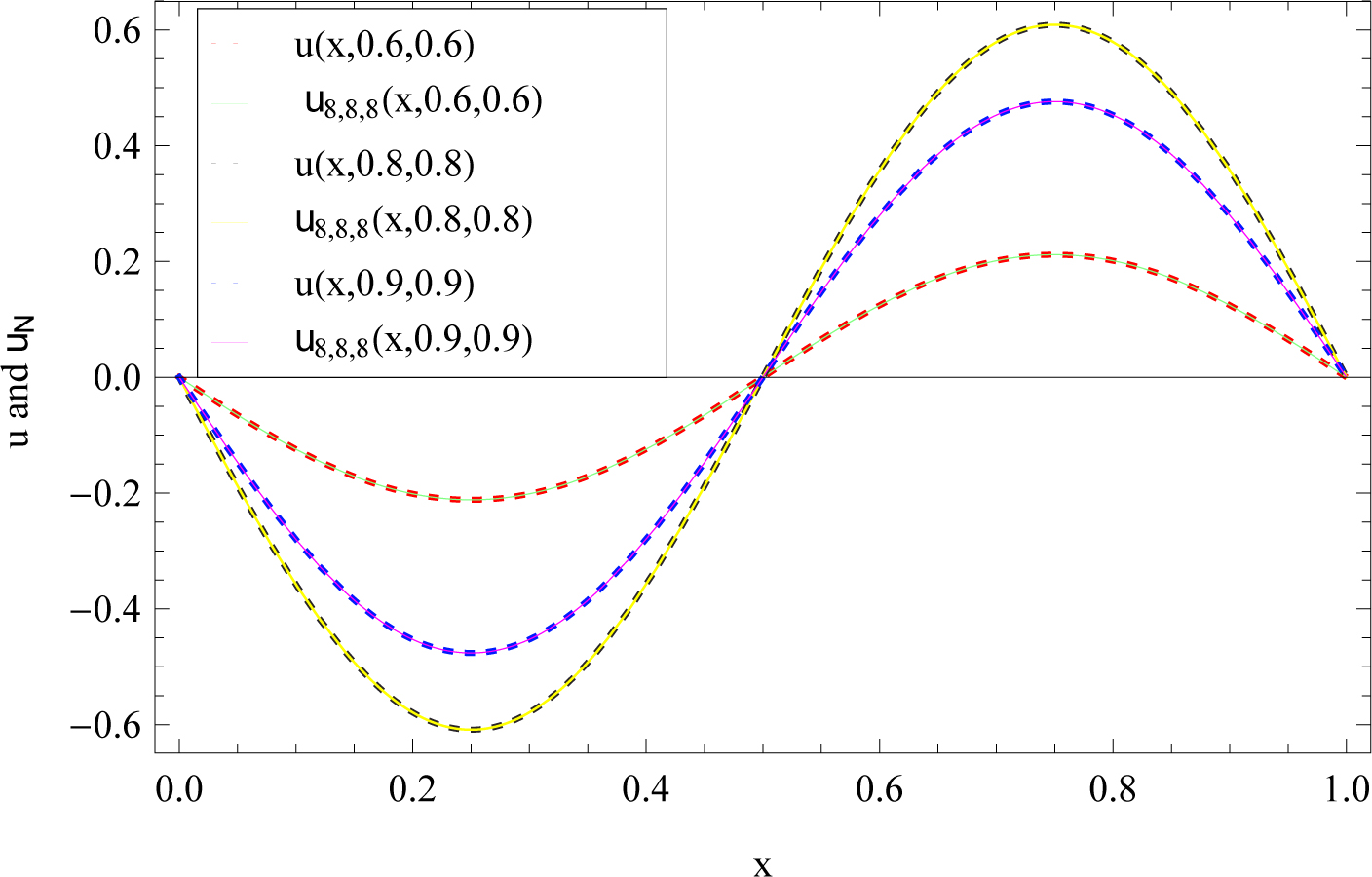
x-direction curves of exact and numerical solutions for Example 4 with
6 Conclusion
By means of SJ-GL-C and SJ-GR-C schemes, we have introduced a space-time spectral algorithm for solving T-FTTEs . According to the numerical results obtained above, we can concluded the high accuracy of our technique. Numerical examples were given to confirm the rightness and reliability of our method. The results display the accuracy of the novel method.
References
[1] Magin R.L., Fractional Calculus in Bioengineering, Begell House Publishers, 2006.Search in Google Scholar
[2] Metzler R., Klafter J., The restaurant at the end of the random walk: Recent developments in the description of anomalous transport by fractional dynamics, J. Phys. A, 2004, 37, 161–208.10.1088/0305-4470/37/31/R01Search in Google Scholar
[3] Kirchner J.W., Feng X., Neal C., Fractal stream chemistry and its implications for containant transport in catchments, Nature, 2000, 403, 524–526.10.1038/35000537Search in Google Scholar
[4] Baillie R.T., Long memory processes and fractional integration in econometrics, J. Econometrics, 1996, 73, 5–59.10.1016/0304-4076(95)01732-1Search in Google Scholar
[5] Kilbas A.A., Srivastava H.M., Trujillo J.J., Theory and Applications of Fractional Differential Equations, Elsevier, San Diego, 2006.Search in Google Scholar
[6] Podlubny I., Fractional Differential Equations, in: Mathematics in Science and Engineering, Academic Press Inc., San Diego, CA, 1999.Search in Google Scholar
[7] Wang L., Ma Y., Meng Z., Haar wavelet method for solving fractional partial differential equations numerically, Appl. Math. Comput., 2014 227, 66–76.10.1016/j.amc.2013.11.004Search in Google Scholar
[8] Ma J., Liu J., Zhou Z., Convergence analysis of moving finite element methods for space fractional differential equations, J. Comput. Appl. Math., 2014, 255, 661–670.10.1016/j.cam.2013.06.021Search in Google Scholar
[9] Doha E.H., Bhrawy A.H., Ezz-Eldien S.S., A new Jacobi operational matrix: An application for solving fractional differential equations, Appl. Math. Model., 2012, 36, 4931–4943.10.1016/j.apm.2011.12.031Search in Google Scholar
[10] Bhrawy A.H., Zaky M.A., A method based on the Jacobi tau approximation for solving multi-term time-space, J. Comput. Phys., 2015, 281, 876–895.10.1016/j.jcp.2014.10.060Search in Google Scholar
[11] Jiang Y.L., Ding X.L., Waveform relaxation methods for fractional differential equations with the Caputo derivatives, J. Comput. Appl. Math., 2013, 238, 51–67.10.1016/j.cam.2012.08.018Search in Google Scholar
[12] Wang H., Du N., Fast alternating-direction finite difference methods for three-dimensional space-fractional diffusion equations, J. Comput. Phys., 2014, 258, 305–318.10.1016/j.jcp.2013.10.040Search in Google Scholar
[13] Yin F., Song J., Leng H., Lu F., Couple of the variational iteration method and fractional-order Legendre functions method for fractional differential equations, Sci. World J., 2014, 928765-9.10.1155/2014/928765Search in Google Scholar PubMed PubMed Central
[14] Piret C., Hanert E., A radial basis functions method for fractional diffusion equations, J. Comput. Phys., 2012, 238, 71–81.10.1016/j.jcp.2012.10.041Search in Google Scholar
[15] Shen S., Liu F., Anh V., Turner I., Chen J., A characteristic difference method for the variable-order fractional advection-diffusion equation, Appl. Math. Comput., 2013, 42, 371–386.10.1007/s12190-012-0642-0Search in Google Scholar
[16] Canuto C., Hussaini M.Y., Quarteroni A., Zang T.A., Spectral Methods: Fundamentals in Single Domains. Springer-Verlag, New York 2006.10.1007/978-3-540-30726-6Search in Google Scholar
[17] Bhrawy A.H., A Jacobi spectral collocation method for solving multi-dimensional nonlinear fractional sub-diffusion equations, Numer. Algorithms, 2016, DOI:10.1007/s11075-015-0087-2.Search in Google Scholar
[18] Bhrawy A.H., Zaky M.A., Numerical algorithm for the variable-order Caputo fractional functional differential equation, Nonlinear Dynam., 2016, DOI:10.1007/s11071-016-2797-y.Search in Google Scholar
[19] Bhrawy A.H., Zaky M.A., Machado J.T., Numerical Solution of the Two-sided Space-Time Fractional Telegraph Equation via Chebyshev Tau Approximation, J. Optimiz Theory App., 2016, DOI:10.1007/s10957-016-0863-8.Search in Google Scholar
[20] Bhrawy A.H., Zaky M.A., Shifted fractional-order Jacobi orthogonal functions: Application to a system of fractional differential equations, Appl. Math. Modell., 2016, 40(2), 832–845.10.1016/j.apm.2015.06.012Search in Google Scholar
[21] Bhrawy A.H., An efficient Jacobi pseudospectral approximation for nonlinear complex generalized Zakharov system, Appl. Math. Comput., 2014, 247, 30–46.10.1016/j.amc.2014.08.062Search in Google Scholar
[22] Doha E.H., Bhrawy A.H., Abdelkawy M.A., Gorder R.A.V., Jacobi-Gauss-Lobatto collocation method for the numerical solution of 1 + 1 nonlinear Schrödinger equations, J. Comput. Phys., 2014, 261, 244–255.10.1016/j.jcp.2014.01.003Search in Google Scholar
[23] Xu Q., Hesthaven J.S., Stable multi-domain spectral penalty methods for fractional partial differential equations, J. Comput. Phys., 2014, 257, 241–258.10.1016/j.jcp.2013.09.041Search in Google Scholar
[24] Bhrawy A.H., Zaky M.A., Baleanu D., New numerical approximations for space-time fractional Burgers’ equations via a Legendre spectral-collocation method, Rom. Rep. Phys., 2015, 67(2), 340–349.Search in Google Scholar
[25] Ma X., Huang C., Spectral collocation method for linear fractional integro-differential equations, Appl. Math. Modell., 2014, 38, 1434–1448.10.1016/j.apm.2013.08.013Search in Google Scholar
[26] Bhrawy A.H., Doha E.H., Ezz-Eldien S.S., R.A.V. Gorder, A new Jacobi spectral collocation method for solving 1+1 fractional Schrödinger equations and fractional coupled Schrödinger systems, Eur. Phys. J. Plus, 2014, 129, 260.10.1140/epjp/i2014-14260-6Search in Google Scholar
[27] Bhrawy A.H., Doha E.H., Ezz-Eldien S.S. and Abdelkawy M.A., A numerical technique based on the shifted Legendre polynomials for solving the time-fractional coupled KdV equation, Calcolo, 2015, DOI: 10.1007/s10092-014-0132-x.Search in Google Scholar
[28] Tricomi F., Sulle equazioni lineari alle derivate parziali di secondo ordine, di tipomisto. Rend. R. Accad. Lincei, Cl. Sci. Fis. Mat. Natur., 1923, 5, 134–247.Search in Google Scholar
[29] Frankl F., On the problems of Chaplygin for mixed sub- and supersonic flows. Bull. Acad. Sci. USSR Ser. Math., 1945, 9, 121–143.Search in Google Scholar
[30] Zhang X., Liu J., Wen J., Tang B., He Y., Analysis for one-dimensional time-fractional Tricomi-type equations by LDG methods, Numer. Algor., 2013, 63, 143–164.10.1007/s11075-012-9617-3Search in Google Scholar
[31] Bers L., Mathematical aspects of subsonic and transonic gas dynamics. In: Surveys in Applied Mathematics, vol. 3. Wiley/Chapman & Hall, New York, London 1958.Search in Google Scholar
[32] Cole J.D., Cook L.P., Transonic Aerodynamics. Elsevier/North-Holland, Amsterdam/New York, 1986.Search in Google Scholar
[33] Germain P., The Tricomi equation, its solutions and their applications in fluid dynamics. In: Tricomi’s Ideas and Contemporary Applied Mathematics, Rome/Turin (1997). In: Atti Convegni Lincei, Accad. Naz. Lincei, Rome, 1998, 147, 7–26.Search in Google Scholar
[34] Morawetz C., Mixed equations and transonic flow. J. Hyperbol Differ. Eq., 2004, 1, 1–26.10.1142/S0219891604000081Search in Google Scholar
[35] Nocilla S., Applications and developments of the Tricomi equation in the transonic aerodynamics. In: Mixed Type Equations, Teubner-Texte Math., Teubner, Leipzig, 1986, 90, 216–241.Search in Google Scholar
[36] Zhang X., Huang P., Feng X., Wei L., Finite element method for two-dimensional time-fractional tricomi-type equations, Numer. Meth. Part. D.E., 2013, 29(4), 1081–1096.10.1002/num.21745Search in Google Scholar
© 2016 M.A. Abdelkawy et al., published by De Gruyter Open
This work is licensed under the Creative Commons Attribution-NonCommercial-NoDerivatives 3.0 License.
Articles in the same Issue
- Regular articles
- Speeding of α Decay in Strong Laser Fields
- Regular articles
- Multi-soliton rational solutions for some nonlinear evolution equations
- Regular articles
- Thin film flow of an Oldroyd 6-constant fluid over a moving belt: an analytic approximate solution
- Regular articles
- Bilinearization and new multi-soliton solutions of mKdV hierarchy with time-dependent coefficients
- Regular articles
- Duality relation among the Hamiltonian structures of a parametric coupled Korteweg-de Vries system
- Regular articles
- Modeling the potential energy field caused by mass density distribution with Eton approach
- Regular articles
- Climate Solutions based on advanced scientific discoveries of Allatra physics
- Regular articles
- Investigation of TLD-700 energy response to low energy x-ray encountered in diagnostic radiology
- Regular articles
- Synthesis of Pt nanowires with the participation of physical vapour deposition
- Regular articles
- Quantum discord and entanglement in grover search algorithm
- Regular articles
- On order statistics from nonidentical discrete random variables
- Regular articles
- Charmed hadron photoproduction at COMPASS
- Regular articles
- Perturbation solutions for a micropolar fluid flow in a semi-infinite expanding or contracting pipe with large injection or suction through porous wall
- Regular articles
- Flap motion of helicopter rotors with novel, dynamic stall model
- Regular articles
- Impact of severe cracked germanium (111) substrate on aluminum indium gallium phosphate light-emitting-diode’s electro-optical performance
- Regular articles
- Slow-fast effect and generation mechanism of brusselator based on coordinate transformation
- Regular articles
- Space-time spectral collocation algorithm for solving time-fractional Tricomi-type equations
- Regular articles
- Recent Progress in Search for Dark Sector Signatures
- Regular articles
- Recent progress in organic spintronics
- Regular articles
- On the Construction of a Surface Family with Common Geodesic in Galilean Space G3
- Regular articles
- Self-healing phenomena of graphene: potential and applications
- Regular articles
- Viscous flow and heat transfer over an unsteady stretching surface
- Regular articles
- Spacetime Exterior to a Star: Against Asymptotic Flatness
- Regular articles
- Continuum dynamics and the electromagnetic field in the scalar ether theory of gravitation
- Regular articles
- Corrosion and mechanical properties of AM50 magnesium alloy after modified by different amounts of rare earth element Gadolinium
- Regular articles
- Genocchi Wavelet-like Operational Matrix and its Application for Solving Non-linear Fractional Differential Equations
- Regular articles
- Energy and Wave function Analysis on Harmonic Oscillator Under Simultaneous Non-Hermitian Transformations of Co-ordinate and Momentum: Iso-spectral case
- Regular articles
- Unification of all hyperbolic tangent function methods
- Regular articles
- Analytical solution for the correlator with Gribov propagators
- Regular articles
- A New Algorithm for the Approximation of the Schrödinger Equation
- Regular articles
- Analytical solutions for the fractional diffusion-advection equation describing super-diffusion
- Regular articles
- On the fractional differential equations with not instantaneous impulses
- Topical Issue: Uncertain Differential Equations: Theory, Methods and Applications
- Exact solutions of the Biswas-Milovic equation, the ZK(m,n,k) equation and the K(m,n) equation using the generalized Kudryashov method
- Topical Issue: Uncertain Differential Equations: Theory, Methods and Applications
- Numerical solution of two dimensional time fractional-order biological population model
- Topical Issue: Uncertain Differential Equations: Theory, Methods and Applications
- Rotational surfaces in isotropic spaces satisfying weingarten conditions
- Topical Issue: Uncertain Differential Equations: Theory, Methods and Applications
- Anti-synchronization of fractional order chaotic and hyperchaotic systems with fully unknown parameters using modified adaptive control
- Topical Issue: Uncertain Differential Equations: Theory, Methods and Applications
- Approximate solutions to the nonlinear Klein-Gordon equation in de Sitter spacetime
- Topical Issue: Uncertain Differential Equations: Theory, Methods and Applications
- Stability and Analytic Solutions of an Optimal Control Problem on the Schrödinger Lie Group
- Topical Issue: Recent Developments in Applied and Engineering Mathematics
- Logical entropy of quantum dynamical systems
- Topical Issue: Recent Developments in Applied and Engineering Mathematics
- An efficient algorithm for solving fractional differential equations with boundary conditions
- Topical Issue: Recent Developments in Applied and Engineering Mathematics
- A numerical method for solving systems of higher order linear functional differential equations
- Topical Issue: Recent Developments in Applied and Engineering Mathematics
- Nonlinear self adjointness, conservation laws and exact solutions of ill-posed Boussinesq equation
- Topical Issue: Recent Developments in Applied and Engineering Mathematics
- On combined optical solitons of the one-dimensional Schrödinger’s equation with time dependent coefficients
- Topical Issue: Recent Developments in Applied and Engineering Mathematics
- On soliton solutions of the Wu-Zhang system
- Topical Issue: Recent Developments in Applied and Engineering Mathematics
- Comparison between the (G’/G) - expansion method and the modified extended tanh method
- Topical Issue: Recent Developments in Applied and Engineering Mathematics
- On the union of graded prime ideals
- Topical Issue: Recent Developments in Applied and Engineering Mathematics
- Oscillation criteria for nonlinear fractional differential equation with damping term
- Topical Issue: Recent Developments in Applied and Engineering Mathematics
- A new method for computing the reliability of consecutive k-out-of-n:F systems
- Topical Issue: Recent Developments in Applied and Engineering Mathematics
- A time-delay equation: well-posedness to optimal control
- Topical Issue: Recent Developments in Applied and Engineering Mathematics
- Numerical solutions of multi-order fractional differential equations by Boubaker polynomials
- Topical Issue: Recent Developments in Applied and Engineering Mathematics
- Laplace homotopy perturbation method for Burgers equation with space- and time-fractional order
- Topical Issue: Recent Developments in Applied and Engineering Mathematics
- The calculation of the optical gap energy of ZnXO (X = Bi, Sn and Fe)
- Special Issue: Advanced Computational Modelling of Nonlinear Physical Phenomena
- Analysis of time-fractional hunter-saxton equation: a model of neumatic liquid crystal
- Special Issue: Advanced Computational Modelling of Nonlinear Physical Phenomena
- A certain sequence of functions involving the Aleph function
- Special Issue: Advanced Computational Modelling of Nonlinear Physical Phenomena
- On negacyclic codes over the ring ℤp + uℤp + . . . + uk + 1 ℤp
- Special Issue: Advanced Computational Modelling of Nonlinear Physical Phenomena
- Solitary and compacton solutions of fractional KdV-like equations
- Special Issue: Advanced Computational Modelling of Nonlinear Physical Phenomena
- Regarding on the exact solutions for the nonlinear fractional differential equations
- Special Issue: Advanced Computational Modelling of Nonlinear Physical Phenomena
- Non-local Integrals and Derivatives on Fractal Sets with Applications
- Special Issue: Advanced Computational Modelling of Nonlinear Physical Phenomena
- On the solutions of electrohydrodynamic flow with fractional differential equations by reproducing kernel method
- Special issue on Information Technology and Computational Physics
- On uninorms and nullnorms on direct product of bounded lattices
- Special issue on Information Technology and Computational Physics
- Phase-space description of the coherent state dynamics in a small one-dimensional system
- Special issue on Information Technology and Computational Physics
- Automated Program Design – an Example Solving a Weather Forecasting Problem
- Special issue on Information Technology and Computational Physics
- Stress - Strain Response of the Human Spine Intervertebral Disc As an Anisotropic Body. Mathematical Modeling and Computation
- Special issue on Information Technology and Computational Physics
- Numerical solution to the Complex 2D Helmholtz Equation based on Finite Volume Method with Impedance Boundary Conditions
- Special issue on Information Technology and Computational Physics
- Application of Genetic Algorithm and Particle Swarm Optimization techniques for improved image steganography systems
- Special issue on Information Technology and Computational Physics
- Intelligent Chatter Bot for Regulation Search
- Special issue on Information Technology and Computational Physics
- Modeling and optimization of Quality of Service routing in Mobile Ad hoc Networks
- Special issue on Information Technology and Computational Physics
- Resource management for server virtualization under the limitations of recovery time objective
- Special issue on Information Technology and Computational Physics
- MODY – calculation of ordered structures by symmetry-adapted functions
- Special issue on Information Technology and Computational Physics
- Survey of Object-Based Data Reduction Techniques in Observational Astronomy
- Special issue on Information Technology and Computational Physics
- Optimization of the prediction of second refined wavelet coefficients in electron structure calculations
- Special Issue on Advances on Modelling of Flowing and Transport in Porous Media
- Droplet spreading and permeating on the hybrid-wettability porous substrates: a lattice Boltzmann method study
- Special Issue on Advances on Modelling of Flowing and Transport in Porous Media
- POD-Galerkin Model for Incompressible Single-Phase Flow in Porous Media
- Special Issue on Advances on Modelling of Flowing and Transport in Porous Media
- Effect of the Pore Size Distribution on the Displacement Efficiency of Multiphase Flow in Porous Media
- Special Issue on Advances on Modelling of Flowing and Transport in Porous Media
- Numerical heat transfer analysis of transcritical hydrocarbon fuel flow in a tube partially filled with porous media
- Special Issue on Advances on Modelling of Flowing and Transport in Porous Media
- Experimental Investigation on Oil Enhancement Mechanism of Hot Water Injection in tight reservoirs
- Special Issue on Research Frontier on Molecular Reaction Dynamics
- Role of intramolecular hydrogen bonding in the excited-state intramolecular double proton transfer (ESIDPT) of calix[4]arene: A TDDFT study
- Special Issue on Research Frontier on Molecular Reaction Dynamics
- Hydrogen-bonding study of photoexcited 4-nitro-1,8-naphthalimide in hydrogen-donating solvents
- Special Issue on Research Frontier on Molecular Reaction Dynamics
- The Interaction between Graphene and Oxygen Atom
- Special Issue on Research Frontier on Molecular Reaction Dynamics
- Kinetics of the austenitization in the Fe-Mo-C ternary alloys during continuous heating
- Special Issue: Functional Advanced and Nanomaterials
- Colloidal synthesis of Culn0.75Ga0.25Se2 nanoparticles and their photovoltaic performance
- Special Issue: Functional Advanced and Nanomaterials
- Positioning and aligning CNTs by external magnetic field to assist localised epoxy cure
- Special Issue: Functional Advanced and Nanomaterials
- Quasi-planar elemental clusters in pair interactions approximation
- Special Issue: Functional Advanced and Nanomaterials
- Variable Viscosity Effects on Time Dependent Magnetic Nanofluid Flow past a Stretchable Rotating Plate