Quantum chemistry – from the first steps to linear-scaling electronic structure methods

The birth of quantum chemistry

Understanding the reason why atoms form molecules, the maximum number of groups that a given atom may attach to itself, and further the geometrical arrangement of these groups has kept scientists struggling for many decades. In the early 19th century, John Dalton’s pioneering atomic theory provided a quantitative foundation by showing that elements combine in fixed integer ratios. ^{1 , 2} Building on these insights, Jöns J. Berzelius utilized a huge body of analytical data to validate and extend the findings of Dalton. ³ Berzelius’ work was crucial in manifesting the concept that atoms bond in fixed stoichiometric ratios, giving rise to the idea of valency – the bonding capacity of an atom. It took until the middle of the century when August Kekulé proposed in 1857 that carbon is able to form four bonds ⁴ and one year later that carbon atoms can form long chains. ⁵ Independently, Archibald Scott Couper went a step further in his theory published in 1858 by drawing bonds as lines between atomic symbols, explicitly depicting the chemical bond for the first time. ⁶ In 1861, Aleksandr M. Butlerov formalized the concept of chemical structure, declaring that the properties of a compound are determined not just by the types of atoms it contains but also by how these atoms are arranged and connected. ⁷ A further milestone was achieved another 13 years later in 1874, when Jacobus van’t Hoff ⁸ and Joseph Le Bel ⁹ independently proposed that a compound containing a single carbon atom with four different substituents could exist in two forms that are mirror images of each other when the four carbon bonds are oriented at the corners of a tetrahedron, which can be seen as the beginning of stereochemistry.

Up to this point, very little was known about the nature of the chemical bond; however, this began to change in 1897 when J. J. Thomson discovered the electron. Thomson showed that atoms contain tiny negatively charged particles (electrons) ¹⁰ and by 1904 he proposed the “plum pudding” model of the atom – a positive sphere studded with electrons – in which electrostatic forces hold the electrons in place, manifesting the idea that the nature of a chemical bond is essentially electronic. ¹¹ Indeed, in 1916 Gilbert N. Lewis conceptualized chemical bonds via shared electron pairs (“electron pair bond”), known today as covalent bonds. ¹² Furthermore, he formulated the “octet rule”, the idea that atoms gain chemical stability by achieving an electron configuration resembling noble gases (usually eight electrons in the valence shell). Although simplistic, this provided remarkable predictive power, especially for organic molecules and main-group compounds and the concepts became foundational for modern chemical bonding and electronic structure theory.

However, these static electron-pair models faced serious theoretical issues. From a classical physics standpoint, if electrons are simply point charges, two electrons held between two positive nuclei should not remain fixed in space. Earnshaw’s theorem ¹³ states that it is impossible to maintain a stable equilibrium of static electric charges under electrostatic forces alone. In other words, modeling a bond as two stationary electrons shared between atoms would be unstable – the electrons should either collapse onto the nuclei or fly apart. Furthermore, this model was a purely formal description and did not tell anything about what the sharing of electrons means and how it arises.

The birth of quantum mechanics in the early 20th century, with the pioneering works of Max Planck, ¹⁴ Albert Einstein, ¹⁵ Niels Bohr, ^{16 , 17 , 18} Werner Heisenberg, ^{19 , 20 , 21 , 22} Erwin Schrödinger, ^{23 , 24 , 25 , 26} Paul A. M. Dirac, ^{27 , 28 , 29 , 30} Wolfgang Pauli, ^{31 , 32} among others, marked a turning point in this regard. Niels Bohr’s description of the atom was the first one to mix classical mechanics, describing the electrons as point charges orbiting the nucleus, with quantum mechanical conditions, so that the angular momentum of the electrons could only take discrete (quantized) values, leading to orbits with definite energies. ^{16 , 17 , 18} Although it was a great advancement that successfully explained the spectrum of the hydrogen atom, it suffered from severe inadequacies. It struggled with multi-electron atoms and offered no rigorous explanation for chemical bonding between atoms. Furthermore, the concept of fixed electron orbits is inconsistent with classical mechanics, which would suggest that moving charges, such as electrons, should radiate energy and eventually spiral into the nucleus. It was hence soon recognized that Bohr’s approach, while revolutionary, was not the final answer: it needed the full machinery of the emerging quantum theory.

A purely quantum mechanical description, famously introduced by Erwin Schrödinger in 1926, which describes the electrons as waves, solved that problem, and quantum mechanics for the first time allowed for a coherent and inclusive theory of molecular structure. ^{23 , 24 , 25 , 26} In 1927, Walter Heitler and Fritz London published a landmark quantum-mechanical study of the hydrogen molecule, demonstrating that a stable bound state emerges from the quantum-mechanical treatment. ³³ This was the first ab initio (first-principles) explanation of a covalent bond and marked the beginning of quantum chemistry (QC). In 1929, Paul A. M. Dirac famously stated “The underlying physical laws necessary for the mathematical theory of a large part of physics and the whole of chemistry are thus completely known, and the difficulty is only that the exact application of these laws leads to equations much too complicated to be soluble”. ³⁰ Therefore, the challenge shifted from uncovering the fundamental laws of chemistry to developing feasible new approaches for their approximation.

Approximating the electronic Schrödinger equation

Traditionally, quantum chemistry focuses on solving the time-independent Schrödinger equation ³⁴ within the Born-Oppenheimer approximation ³⁵

with the molecular Hamiltonian H ̂ , the electronic wavefunction Ψ, the total energy of the chemical system E, the set of electronic coordinates r e ≡ ( r 1 , … , r N el ) , and the set of fixed nuclear coordinates R n ≡ ( R 1 , … , R N at ) . The fundamental importance of the total energy is evident from its central role in the Schrödinger equation; however, its physical meaning remains rather abstract, as it represents the energy released when the electrons and nuclei are brought together from infinity to form the molecule. From a chemical perspective, energy differences are of greater practical relevance, as they play the dominant role in nearly all molecular phenomena. Chemical bonds form as a result of a decrease in the total energy relative to that of the separated atoms, and molecular geometries – bond angles and bond lengths – adjust to minimize the energy. Accordingly, the theory of molecular structure can, in broad terms, be regarded as a theory of calculating energies and, more importantly, their differences.

Early approximations to the Schrödinger equation were pioneered by Hartree in 1928. ³⁶ However, as was pointed out independently by J. C. Slater ³⁷ and V. A. Fock ³⁸ in 1930, the Hartree method did not account for the antisymmetry requirement of fermionic wavefunctions, ^{20 , 28} violating the Pauli exclusion principle introduced in 1925, which states that two electrons cannot share the same set of quantum numbers. ^{31 , 32} Fock solved the problem of fulfilling the antisymmetry requirement of the wavefunction by approximating it with a single Slater determinant ^{20 , 28 , 37} built from one-particle wavefunctions – the molecular orbitals – resulting in the Hartree–Fock (HF) method. ^{36 , 38} Yet, due to the complexity of the first formulation, the HF method was rarely employed initially, with simpler empirical methods dominating. A major breakthrough came with the algebraization of the problem in 1951, resulting in the Roothaan–Hall equations ^{39 , 40}

where F denotes the Fock matrix, S the overlap matrix, C the matrix of coefficients to expand the molecular orbitals in a fixed basis of atomic orbitals, and ϵ denotes the matrix of orbital energies. These equations, solved by diagonalizing the Fock matrix in an orthogonolized basis, transformed the HF method into a practically viable computational approach and, combined with the advent of digital computers, dramatically increased the accessibility and popularity of the HF method, laying the foundation of modern ab initio quantum chemistry.

The HF method was a milestone in the development of quantum chemistry, however, it was still far away from an exact theory. Although same-spin electrons are “correlated” to some extent in the HF method due to the antisymmetry of the employed wavefunction, opposite-spin electrons are completely uncorrelated. To account for these missing correlation effects, which are crucial for the accurate description of the electronic structure, many so-called post-HF methods have been developed. Although the accuracy of these methods can, in principle, be systematically increased even up to numerical exactness in the full configuration interaction (FCI) or the coupled-cluster (CC) method, as illustrated in Fig. 1, the increase of the computational cost is extremely steep, ⁴¹ limiting the applicability of highly accurate wavefunction methods to molecular systems on the few-atom scale.

Fig. 1:

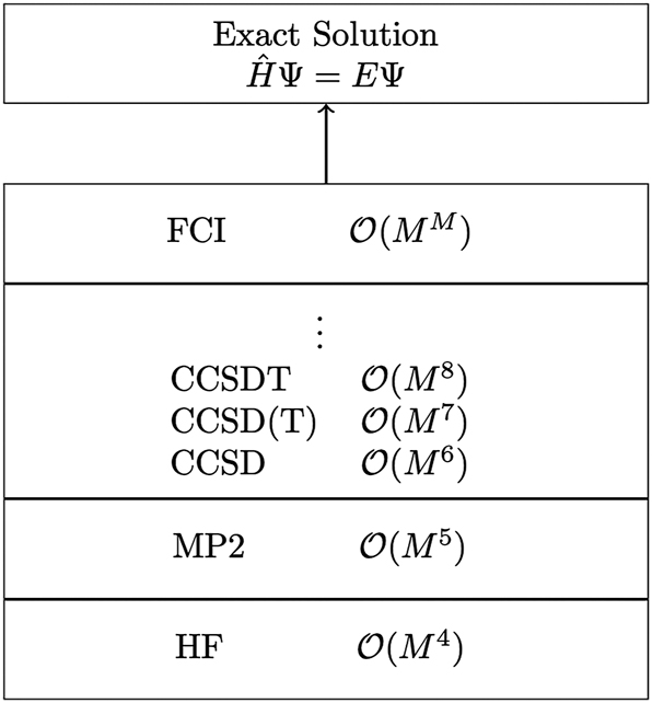
Schematic illustration of a modern hierarchy of wavefunction-based methods, along with the formal scaling behavior of their computational cost with respect to system size M.

The primary reason why these post-HF methods are so computationally expensive can be rationalized by the fact that they rely on approximating the electronic wavefunction – a highly complex function depending on the spatial- and spin-coordinates of all electrons in the system. From a mathematical perspective, representing an antisymmetric function with N variables exactly, requires a linear combination of all unique N-variable Slater determinants formed from a complete set of one-variable functions. Even for a finite set of one-variable functions the number of unique Slater determinants scales combinatorially, making such an approach computationally extremely expensive. Still, this is precisely what is done in the FCI method (within a finite basis), where the name originates from the fact that each Slater determinant formed from a specific set of molecular orbitals is called a configuration.

An alternative approach to solving the Schrödinger equation emerged in 1964 and 1965, when P. Hohenberg, W. Kohn, and L. J. Sham developed (Kohn–Sham) density functional theory ((KS-)DFT). ^{42 , 43} DFT circumvents the complexity of the many-electron wavefunction by employing the electron density as the central quantity – a significantly simpler quantity that depends only on three spatial variables. Although the initial adoption of DFT within the quantum chemistry community was slow, it has since evolved into the most successful electronic structure approach in most areas of quantum chemistry due to its excellent cost to performance ratio.

The balance between accuracy and efficiency is a decisive factor in the success of any quantum chemical method and, therefore, reducing the computational cost of a given quantum chemical method while retaining its accuracy is of central importance for its applicability. A crucial metric in this respect is the so-called scaling behavior, which relates the increase in the computational cost with the growth of the system size. The next section is dedicated to illustrating some techniques to reduce this scaling behavior to linear.

Linear-scaling electronic structure methods

The development of linear-scaling methods represents a crucial advancement in quantum chemistry, enabling the treatment of large molecular systems. As mentioned earlier, the scaling behavior of a quantum chemical method relates the increase in computational cost with the growth of the system size. For example, in conventional formulations of HF and DFT the computational cost scales formally quartic, M ⁴, with M being a measure of the system size. This means that increasing the system size by a factor of 10 results in a 10 000-fold increase in computational effort. In contrast, a linear-scaling formulation results only in a 10-fold increase – a notable reduction of the computational cost and a crucial step when aiming for large systems. But where does the scaling behavior of a quantum chemical method come from? And what scaling behavior should be expected?

To answer that question, the molecular Hamiltonian of a given system in atomic units within the Born-Oppenheimer approximation should be considered:

with the nuclear charges Z _A , the total number of electrons N _el, and the total number of atoms N _at. The first term of the Hamiltonian describes the kinetic energy of the electrons, the second term the electrostatic interaction between all the electrons, the third term the electrostatic interaction between the electrons and the nuclei, and finally, the last term the electrostatic interaction between the different nuclei. Since the nuclei are considered as fixed charges within the Born-Oppenheimer approximation, the by far most complicated contribution is the electron-electron interaction. On first sight, this interaction does not seem too complicated since it is based on a two-particle operator. The problem is, however, that (in principle) all electrons within the system are correlated with each other, meaning that the interaction of any two electrons also affects all other electrons, leading to a combinatorial complexity of the electronic structure problem with O ( M M ) scaling. Still, it feels only natural that for increasingly large molecules the interactions between individual electrons far apart from each other should become negligibly weak, leading to a constant number of interaction partners for each electron and hence a linear scaling of complexity. Having successfully worked with concepts like localized functional groups and bonds for decades, most organic chemists would likely affirm this statement without hesitation. Therefore, at least in principle and for large enough systems, the development of linear scaling QC methods should be possible. But why do conventional QC methods not account for this? And how can we account for it?

The main problem with conventional QC methods is that their formulations are based on canonical molecular orbitals. These orbitals are delocalized over the entire systems and hence prevent efficient exploitation of locality in the electronic structure. Over the years, many approaches have been proposed and refined to achieve linear scaling, see, e.g. refs. [44], [45], [46 for an overview. Here, we do not aim to provide a full account, but rather focus on approaches that are based on local atomic orbitals – and, in particular, atom-centered Gaussian functions – and the so-called one-particle density matrix P. Although generally applicable, we will illustrate the underlying concepts using the example of DFT.

The equations that need to be solved in (KS-)DFT are analogous to the HF equations and are given by

with the KS-matrix F _KS replacing the Fock matrix F in HF theory. The elements of the overlap matrix S are given by

with the atomic orbitals denoted as χ _μ (r). As the standard choice for the atomic orbital basis is to employ local Gaussian functions, their overlap decreases exponentially and becomes negligible very quickly. This, in turn, leads to a constant number of atomic orbitals χ _ν overlapping with a given atomic orbital χ _μ and hence a linear-scaling number of non-negligible elements in S.

The computationally costly part of Eq. (4) is the formation of the KS-matrix, which is given by

with the one-electron contributions – the kinetic energy and the electron-nuclei interaction – h _core, the Coulomb matrix J, the (HF) exchange matrix K, and exchange-correlation matrix V _xc. Here, γ = 1 for pure KS-DFT and 0 < γ < 1 for hybrid schemes. Further, note that the HF method is obtained if γ = 0 and correlation is neglected; hence, the following discussion is also valid for the HF method.

As mentioned earlier, the main complexity of the electronic structure problem lies in the electron-electron interaction described by J[P], K[P], and V _xc[γ, P]. Let us start with the Coulomb part, which is given by

with the total number of basis functions N _bas and the two-electron four-center integrals

The evaluation of these integrals formally scales as M ⁴, but an asymptotic O ( M 2 ) scaling is easily obtained by accounting for the exponentially decreasing overlap of the atomic orbital pairs with techniques like, e.g., Schwarz screening. ⁴⁷ However, the two atomic orbital pairs μν and λσ are coupled by the slowly decaying 1 r 12 operator, necessitating more sophisticated strategies to further lower the scaling behavior.

The first and nowadays established linear-scaling method for the computation of the Coulomb matrix is the continuous fast-multipole method (CFMM) by White et al. ^{48 , 49} The key idea of this approach is to divide the molecule into small regions or “boxes” that group nearby charge distributions. Interactions are then classified based on distance: nearby charges form the “near field” (NF) and are calculated using standard methods, while distant charges make up the “far field” (FF) and are efficiently approximated using multipole expansions:

In essence, fine grains are used for the description of close interactions and coarse grains for distant ones. Because each region only directly interacts with a limited number of neighbors, both near- and far-field calculations can be performed with an effort that grows only linearly with system size. In this respect, evaluating the NF part is typically by far the most demanding; thus, various methods have been proposed to reduce the prefactor of the evaluation. The J-engine method developed by White et al., ⁵⁰ for instance, sums the density matrix directly into the Gaussian formulas of the four-center two-electron integrals, constructing the Coulomb matrix without explicitly forming the full set of two-electron integral intermediates. Another widely used approach, known as RI-J, ⁵¹ employs the resolution-of-the-identity approximation to factorize the four-center two-electron integrals into two- and three-center terms, thereby speeding up the computation of the Coulomb matrix. Both methods can also be applied outside the CFFM approach; however, in that case, they scale as O ( M 2 ) .

Let us now turn to the evaluation of the exchange matrix which is given by

(10)

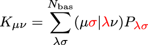
Compared to the evaluation of the Coulomb matrix, the only difference is that now the two atomic orbital pairs μσ and λν are coupled by the one-particle density matrix (highlighted in red). The downside is that the CFMM technique outlined above is not applicable anymore. The advantage, however, is that the one-particle density matrix can be interpreted as a measure for the delocalization of a given system: it is dense for delocalized electronic structures, but it is sparse, i.e., scales linearly for local electronic structures. Thus, for local electronic structures, the number of significant elements within the exchange matrix naturally scales linearly with the system size.

Today, one of the most established methods to exploit this sparsity in the one-particle density matrix and to achieve a linear-scaling computation of the exchange matrix is the so-called LinK method, introduced by Ochsenfeld et al. in 1998. ⁵² The LinK method is designed in such a way that it minimizes the screening overhead, making it competitive with conventional approaches even for small systems. To further reduce the prefactor of the K-matrix computation, several seminumerical approaches have been developed, where one integral of the two-electron integrals is computed numerically on a grid, and the other one is evaluated analytically. For example, Friesner et al. developed the pseudospectral method, ⁵³ Neese et al. introduced the “chains-of-spheres exchange” (COSX) method, ⁵⁴ and Laqua et al. proposed a seminumerical counterpart to the LinK method, the linear-scaling sn-LinK approach. ⁵⁵ An illustrative comparison of the computational cost of the conventional, LinK, seminumerical, and sn-LinK approaches is shown in Fig. 2.

Fig. 2:

Execution time for a single exchange-matrix build using analytical integration (red) with [squares] and without [circles] screening, and seminumerical integration (green) with [triangles] and without [diamonds] screening. Note that the exponentially decreasing overlap of the atomic orbital pairs was accounted for in all algorithms (shell-pair screening). Calculations were performed for DNA systems of increasing length with the def2-TZVP basis set on two AMD EPYC 7302 CPUs (32 cores, 3.0 GHz). The data point marked with an asterisk was extrapolated due to memory limitations.

Besides extremely efficient exchange matrix builds with fully controlled accuracy, the sn-LinK method further enables gradient evaluations at almost no additional cost. ⁵⁶ Combined with graphics processing unit (GPU) acceleration, the sn-LinK method was shown to enable ab initio molecular dynamics (AIMD) simulations with speedups of up to three orders of magnitude compared to conventional approaches, ⁵⁶ opening the door for investigations of large and complex systems.

The final contribution to the electron-electron interaction is the exchange-correlation matrix V _xc. It is the matrix representation of the exchange-correlation potential, which, in turn, is the derivative of the exchange-correlation energy with respect to the electron density ρ(r)

The exchange-correlation energy lies at the heart of KS-DFT and tries to approximate all the unknowns of the system. For the most common functionals leading to a KS-matrix of the form shown in Eq. (6), the exchange-correlation energy is a (semi-)local functional of the electron density ρ(r) and its first (and sometimes also its second) derivative. The important point is that the integration shown in Eq. (11) is typically performed numerically, using a molecular grid built from separate atomic grids, making the total number of grid points scale linearly with system size. To evaluate the functional, the electron density (and also its derivatives) is calculated for each grid point according to

Due to the locality of the Gaussian-type atomic orbitals χ _μ (r), the electron density remains local even for dense one-particle density matrices P, enabling a linear scaling evaluation of V _xc.

Having dealt with all the electron-electron contributions entering the KS-matrix (Eq. (6)), only the one-electron contributions remain. The kinetic part only includes overlap-type integrals, which readily enables a linear-scaling evaluation due to the local nature of the atomic orbitals. The electrostatic interactions between the electrons and the nuclei show the slow 1 r decay just like the interactions between the electrons do, leading to a quadratic scaling behavior. However, the scaling can be reduced to linear using the same strategies described earlier for the Coulomb matrix.

In this section, we presented approaches that enable efficient, linear-scaling computations of DFT and HF energies, allowing for the description of systems that were previously out of reach. We note again, that DFT was chosen merely as an illustrative example, owing to its importance in the quantum chemistry community; however, similar challenges and solutions to those discussed here also arise in other quantum-chemical approaches aiming at exact solutions of the Schrödinger equation.

Furthermore, it should be noted that the presented techniques are not limited to energy computations, but can also be applied to, e.g., the evaluation of molecular properties, typically computed as energy derivatives with respect to one or more perturbations. Such properties include nuclear gradients, ^{57 , 58 , 59 , 60 , 61 , 62} hyperfine coupling constants, ⁶¹ or higher order properties ^{63 , 64} like g-tensors. ⁶⁵ Another important example of such molecular properties are nuclear magnetic resonance (NMR) shielding constants, which can be computed as the mixed second derivative of the energy with respect to the nuclear magnetic moments and the external magnetic field. The development of accurate and efficient computational methods for predicting NMR parameters is essential, as these methods provide an invaluable link to experiment. Here, linear-scaling NMR formulations based on DFT and HF have allowed for the computation of molecular systems with over 1000 atoms. ^{66 , 67} However, in some cases the accuracy obtained with HF or DFT is not sufficient and one has to turn to more advanced QC methods. As mentioned above, such high level methods come with a significant computational cost, which makes the development of low-scaling techniques especially important. One method we would like to mention in this context is the random phase approximation, a post-KS method that has recently been shown to combine high accuracy with computational efficiency for the computation of NMR shieldings. ^{68 , 69}

Bridging theory and experiment is crucial and ultimately determines the practical value of a theoretical approach. In the following section, we briefly introduce the emerging field of autonomous reaction network exploration, which holds great promise in this respect but, due to its substantial computational demands, critically relies on highly efficient, low-scaling methods as, e.g., the ones discussed in the present section.

A new challenge: autonomous reaction network exploration

Over the past decades, quantum chemistry has established itself as an essential tool of modern chemical research, providing detailed insights into molecular processes. It serves as an invaluable complement to experimental work, validating or extending experimental findings. This is particularly true for the investigation of reaction mechanisms, where experimental methods are constrained by limitations in temporal and spatial resolution. Nevertheless, the traditional approach where one hypothesizes a mechanism, computes its energy profile, and then compares it to experimental observations, carries intrinsic limitations and biases. Specifically, such an approach often overlooks the complexity of real systems, including the presence of multiple competing reactions and dynamic equilibria among intermediates. Consequently, computational studies focusing only on a single reaction pathway may provide an incomplete or even misleading view. Addressing this shortcoming requires a more comprehensive strategy: an extensive exploration of the full reaction network, encompassing both productive and non-productive pathways.

At the heart of every reaction network lies a complex potential energy surface (PES), or, when accounting for finite-temperature effects its thermodynamic counterpart, the free energy surface. This multidimensional hypersurface represents the total energy of the system as a function of nuclear coordinates, where local minima and first-order saddle points correspond to reactants, intermediates, products, and transition states, respectively. Elementary steps are defined as transitions between such minima via a single transition state. ⁷⁰ Since chemical compounds are typically represented by different conformers, each elementary step represents only a part of a broader ensemble of transitions linking different structural arrangements of the compounds. This ensemble, taken together, constitutes a chemical transformation or reaction. ⁷⁰ Reaction pathways on such free energy surfaces are then described by one or more chemical transformations and are characterized not only by their thermodynamics involving the free energy differences between reactants and products, but also by their kinetics as described by transition state theory, ⁷¹ relating reaction rates to activation barriers. As the number of possible reaction pathways grows fast with the size of the investigated molecular system, low-scaling methods become indispensable, especially when exploring the PES by AIMD, where thousands of energy and force evaluations are needed.

The field of autonomous reaction network exploration is still in its infancy and the challenge presented by extensively exploring the N _at-dimensional PES is truly enormous; however, building on the achievements of quantum chemists in the last decades, several promising approaches have been put forward in recent years, including CHEMOTON, ⁷² AutoMeKin, ⁷³ the artificial force induced reaction method by Maeda et al., ⁷⁴ the metadynamics-based approach by Grimme, ⁷⁵ the ab initio Nanoreactor, ⁷⁶ and the hyperreactor dynamics (HRD) method ⁷⁷ developed in our group. Taking the reactor-based approaches as an example, the general principle is to enhance reactivity within the system, or in other words, to accelerate exploration of the PES on achievable timescales at ab initio level, which is desired for an accurate description of the underlying molecular processes. In our HRD approach, this is achieved through the combination of two key concepts: The first concept involves a controlled “boosting” of the PES using so-called hyperdynamics potentials, ^{78 , 79 , 80} which help to prevent the system from becoming trapped in deep energy minima during the exploration process. The second concept employs an external, pressure-inducing piston that increases the probability of interatomic collisions. As the system is compressed, entirely new regions of the PES become accessible and can subsequently be explored. The two concepts are illustrated schematically in Fig. 3.

Fig. 3:

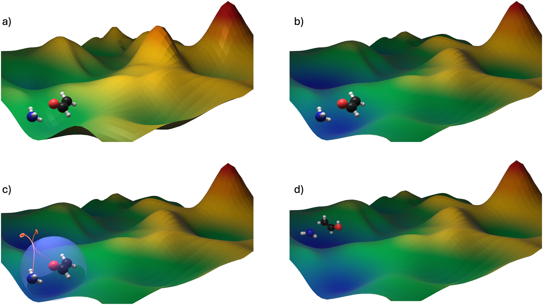
Schematic illustration of (a) the original PES with two reactants forming a local minium (b) the boosted PES (c) the pressure-inducing confinement, enforcing movement on the PES (d) the system in a new local minimum on the boosted PES. Although we typically explore the reactive behavior of larger molecular ensembles, here we focus on visualizing the transition of just two reactants to maintain clarity.

We demonstrated the potential of our HRD approach by simulating the interstellar glycinal and acetamide syntheses at 10 K, ⁷⁷ both regarded as essential precursors for peptide formation. ⁸¹ In these simulations, the expected target molecules were successfully generated. Furthermore, several new reaction pathways were identified, and the formation of N-methylformamide and carbamic acid was observed. Notably, carbamic acid is recognized as the simplest precursor to amino acids, potentially playing a crucial role in chemical evolution. ⁸²

Although there is still a long way to go in the field of autonomous reaction network exploration, this brief example illustrates the predictive power of these new developments and their potential to inform and guide experiments, offering a glimpse of what the near future of quantum chemistry may hold for us.

References

1. Dalton, J. A New System of Chemical Philosophy, Part 1, Vol. 1; S. Russell, 1808.10.5479/sil.324338.39088000885681Search in Google Scholar
2. Dalton, J. A New System of Chemical Philosophy, Part 2, Vol. 2; S. Russell, 1810.Search in Google Scholar
3. Berzelius, J. J. Ann. Philos. 1814, 4, 401.Search in Google Scholar
4. Kekulé, A. Liebigs Ann. 1857, 104, 129.10.1002/jlac.18571040202Search in Google Scholar
5. Kekulé, A. Liebigs Ann. 1858, 106, 129.10.1002/jlac.18581060202Search in Google Scholar
6. Couper, A. S. Lond. Edinb. Dubl. Phil. Mag. 1858, 16, 104; https://doi.org/10.1080/14786445808642541.Search in Google Scholar
7. Butlerov, A. M. Zeitschrift für Chemie 1861, 4, 549.Search in Google Scholar
8. van’t Hoff, J. H. Arch. Neerl. Sci. Exactes Nat. 1874, 9, 445.Search in Google Scholar
9. Le Bel, J. A. Bull. Soc. Chim. Fr. 1874, 22, 337.Search in Google Scholar
10. Thomson, J. J. Lond. Edinb. Dubl. Phil. Mag. 1897, 44, 293; https://doi.org/10.1080/14786449708621070.Search in Google Scholar
11. Thomson, J. J. Lond. Edinb. Dubl. Phil. Mag. 1904, 7, 237.Search in Google Scholar
12. Lewis, G. N. J. Am. Chem. Soc. 1916, 38, 762; https://doi.org/10.1021/ja02261a002.Search in Google Scholar
13. Earnshaw, S. Tran. Camb. Phil. Soc. 1848, 7, 97.Search in Google Scholar
14. Planck, M. Ann. Phys. 1901, 309, 553; https://doi.org/10.1002/andp.19013090310.Search in Google Scholar
15. Einstein, A. Ann. Phys. 1905, 17, 132.10.1086/121638Search in Google Scholar
16. Bohr, N. Lond. Edinb. Dubl. Phil. Mag. 1913, 26, 1.10.1515/crll.1913.143.203Search in Google Scholar
17. Bohr, N. Lond. Edinb. Dubl. Phil. Mag. 1913, 26, 476; https://doi.org/10.1080/14786441308634993.Search in Google Scholar
18. Bohr, N. Lond. Edinb. Dubl. Phil. Mag. 1913, 26, 857; https://doi.org/10.1080/14786441308635031.Search in Google Scholar
19. Heisenberg, W. Z. Phys. 1925, 33, 879; https://doi.org/10.1007/bf01328377.Search in Google Scholar
20. Heisenberg, W. Z. Phys. 1926, 38, 411; https://doi.org/10.1007/bf01397160.Search in Google Scholar
21. Born, M.; Heisenberg, W.; Jordan, P. Z. Phys. 1926, 35, 557; https://doi.org/10.1007/bf01379806.Search in Google Scholar
22. Heisenberg, W. Z. Phys. 1927, 43, 172; https://doi.org/10.1007/bf01397280.Search in Google Scholar
23. Schödinger, E. Ann. Phys. 1926, 79, 361.Search in Google Scholar
24. Schödinger, E. Ann. Phys. 1926, 79, 489.10.1007/978-3-642-90885-9_13Search in Google Scholar
25. Schödinger, E. Ann. Phys. 1926, 80, 437.10.1002/mmnd.192619260108Search in Google Scholar
26. Schödinger, E. Ann. Phys. 1926, 81, 109.Search in Google Scholar
27. Dirac, P. A. M. Proc. R. Soc. Lon. Ser. Math. Phys. Sci. 1925, 109, 642.10.1098/rspa.1925.0150Search in Google Scholar
28. Dirac, P. A. M.; Fowler, R. H. Proc. R. Soc. Lon. Ser. Math. Phys. Sci. 1926, 112, 661.Search in Google Scholar
29. Dirac, P. A. M. Proc. R. Soc. Lon. Ser. Math. Phys. Sci. 1928, 117, 610.10.1098/rspa.1928.0023Search in Google Scholar
30. Dirac, P. A. M. Proc. R. Soc. Lon. Ser. Math. Phys. Sci. 1929, 123, 714.10.1098/rspa.1929.0094Search in Google Scholar
31. Pauli, W. Z. Phys. 1925, 31, 765; https://doi.org/10.1007/bf02980631.Search in Google Scholar
32. Pauli, W. Z. Phys. 1925, 31, 373; https://doi.org/10.1007/bf02980592.Search in Google Scholar
33. Heitler, W.; London, F. Z. Phys. 1927, 44, 455; https://doi.org/10.1007/bf01397394.Search in Google Scholar
34. Schrödinger, E. Phys. Rev. 1926, 28, 1049.10.1103/PhysRev.28.1049Search in Google Scholar
35. Born, M.; Oppenheimer, R. Ann. Phys. 1927, 389, 457; https://doi.org/10.1002/andp.19273892002.Search in Google Scholar
36. Hartree, D. R. Math. Proc. Camb. Phil. Soc. 1928, 24, 111; https://doi.org/10.1017/s0305004100011920.Search in Google Scholar
37. Slater, J. C. Phys. Rev. 1930, 35, 210; https://doi.org/10.1103/physrev.35.210.2.Search in Google Scholar
38. Fock, V. Z. Phys. 1930, 61, 126; https://doi.org/10.1007/bf01340294.Search in Google Scholar
39. Roothaan, C. C. J. Rev. Mod. Phys. 1951, 23, 69; https://doi.org/10.1103/revmodphys.23.69.Search in Google Scholar
40. Hall, G. G.; Lennard-Jones, J. E. Proc. R. Soc. Lon. Ser. Math. Phys. Sci. 1951, 205, 541.Search in Google Scholar
41. Pople, J. A. Angew. Chem. Int. Ed. 1999, 38, 1894; https://doi.org/10.1002/(sici)1521-3773(19990712)38:13/14<1894::aid-anie1894>3.0.co;2-h.10.1002/(SICI)1521-3773(19990712)38:13/14<1894::AID-ANIE1894>3.0.CO;2-HSearch in Google Scholar
42. Hohenberg, P.; Kohn, W. Phys. Rev. 1964, 136, B864; https://doi.org/10.1103/physrev.136.b864.Search in Google Scholar
43. Kohn, W.; Sham, L. J. Phys. Rev. 1965, 140, A1133; https://doi.org/10.1103/physrev.140.a1133.Search in Google Scholar
44. Kussmann, J.; Beer, M.; Ochsenfeld, C. Wiley Interdiscip. Rev.: Comput. Mol. Sci. 2013, 3, 614; https://doi.org/10.1002/wcms.1138.Search in Google Scholar
45. Werner, H.-J.; Knizia, G.; Krause, C.; Schwilk, M.; Dornbach, M. J. Chem. Theory Comput. 2015, 11, 484; https://doi.org/10.1021/ct500725e.Search in Google Scholar PubMed
46. Schwilk, M.; Ma, Q.; Köppl, C.; Werner, H.-J. J. Chem. Theory Comput. 2017, 13, 3650.10.1021/acs.jctc.7b00554Search in Google Scholar PubMed
47. Häser, M.; Ahlrichs, R. J. Comput. Chem. 1989, 10, 104; https://doi.org/10.1002/jcc.540100111.Search in Google Scholar
48. White, C. A.; Head-Gordon, M. J. Chem. Phys. 1994, 101, 6593; https://doi.org/10.1063/1.468354.Search in Google Scholar
49. White, C. A.; Johnson, B. G.; Gill, P. M.; Head-Gordon, M. Chem. Phys. Lett. 1994, 230, 8; https://doi.org/10.1016/0009-2614(94)01128-1.Search in Google Scholar
50. White, C. A.; Head-Gordon, M. J. Chem. Phys. 1996, 104, 2620; https://doi.org/10.1063/1.470986.Search in Google Scholar
51. Weigend, F. Phys. Chem. Chem. Phys. 2002, 4, 4285; https://doi.org/10.1039/b204199p.Search in Google Scholar
52. Ochsenfeld, C.; White, C. A.; Head-Gordon, M. J. Chem. Phys. 1998, 109, 1663; https://doi.org/10.1063/1.476741.Search in Google Scholar
53. Friesner, R. A. Chem. Phys. Lett. 1985, 116, 39; https://doi.org/10.1016/0009-2614(85)80121-4.Search in Google Scholar
54. Neese, F.; Wennmohs, F.; Hansen, A.; Becker, U. Chem. Phys. 2009, 356, 98; https://doi.org/10.1016/j.chemphys.2008.10.036.Search in Google Scholar
55. Laqua, H.; Kussmann, J.; Ochsenfeld, C. J. Chem. Theory Comput. 2018, 14, 3451; https://doi.org/10.1021/acs.jctc.8b00062.Search in Google Scholar PubMed
56. Laqua, H.; Dietschreit, J. C. B.; Kussmann, J.; Ochsenfeld, C. J. Chem. Theory Comput. 2022, 18, 6010; https://doi.org/10.1021/acs.jctc.2c00509.Search in Google Scholar PubMed
57. Ochsenfeld, C. Chem. Phys. Lett. 2000, 327, 216; https://doi.org/10.1016/s0009-2614(00)00865-4.Search in Google Scholar
58. Shao, Y.; White, C. A.; Head-Gordon, M. J. Chem. Phys. 2001, 114, 6572; https://doi.org/10.1063/1.1357441.Search in Google Scholar
59. Larsen, H.; Helgaker, T.; Olsen, J.; Jørgensen, P. J. Chem. Phys. 2001, 115, 10344; https://doi.org/10.1063/1.1415082.Search in Google Scholar
60. Reine, S.; Krapp, A.; Iozzi, M. F.; Bakken, V.; Helgaker, T.; Pawłowski, F.; Sałek, P. J. Chem. Phys. 2010, 133; https://doi.org/10.1063/1.3459061.Search in Google Scholar PubMed
61. Vogler, S.; Ludwig, M.; Maurer, M.; Ochsenfeld, C. J. Chem. Phys. 2017, 147; https://doi.org/10.1063/1.4990413.Search in Google Scholar PubMed
62. Pinski, P.; Neese, F. J. Chem. Phys. 2019, 150; https://doi.org/10.1063/1.5086544.Search in Google Scholar PubMed
63. Coriani, S.; Høst, S.; Jansík, B.; Thøgersen, L.; Olsen, J.; Jørgensen, P.; Reine, S.; Pawłowski, F.; Helgaker, T.; Sałek, P. J. Chem. Phys. 2007, 126; https://doi.org/10.1063/1.2715568.Search in Google Scholar PubMed
64. Beer, M.; Ochsenfeld, C. J. Chem. Phys. 2008, 128; https://doi.org/10.1063/1.2940731.Search in Google Scholar PubMed
65. Glasbrenner, M.; Vogler, S.; Ochsenfeld, C. J. Chem. Phys. 2019, 150; https://doi.org/10.1063/1.5066266.Search in Google Scholar PubMed
66. Ochsenfeld, C.; Kussmann, J.; Koziol, F. Angew. Chem. 2004, 116, 4585; https://doi.org/10.1002/ange.200460336.Search in Google Scholar
67. Kussmann, J.; Ochsenfeld, C. J. Chem. Phys. 2007, 127, 054103; https://doi.org/10.1063/1.2749509.Search in Google Scholar PubMed
68. Drontschenko, V.; Bangerter, F. H.; Ochsenfeld, C. J. Chem. Theory Comput. 2023, 19, 7542; https://doi.org/10.1021/acs.jctc.3c00542.Search in Google Scholar PubMed
69. Drontschenko, V.; Ochsenfeld, C. J. Phys. Chem. A 2024, 128, 7950; https://doi.org/10.1021/acs.jpca.4c02773.Search in Google Scholar PubMed PubMed Central
70. Unsleber, J. P.; Reiher, M. Ann. Rev. Phys. Chem. 2020, 71, 121; https://doi.org/10.1146/annurev-physchem-071119-040123.Search in Google Scholar PubMed
71. Eyring, H. J. Chem. Phys. 1935, 3, 107; https://doi.org/10.1063/1.1749604.Search in Google Scholar
72. Unsleber, J. P.; Grimmel, S. A.; Reiher, M. J. Chem. Theory Comput. 2022, 18, 5393; https://doi.org/10.1021/acs.jctc.2c00193.Search in Google Scholar PubMed PubMed Central
73. Martínez-Núñez, E.; Barnes, G. L.; Glowacki, D. R.; Kopec, S.; Peláez, D.; Rodríguez, A.; Rodríguez-Fernández, R.; Shannon, R. J.; Stewart, J. J. P.; Tahoces, P. G.; Vazquez, S. A. J. Comput. Chem. 2021, 42, 2036.10.1002/jcc.26734Search in Google Scholar PubMed
74. Maeda, S.; Harabuchi, Y.; Takagi, M.; Taketsugu, T.; Morokuma, K. Chem. Rec. 2016, 16, 2232; https://doi.org/10.1002/tcr.201600043.Search in Google Scholar PubMed
75. Grimme, S. J. Chem. Theory Comput. 2019, 15, 2847; https://doi.org/10.1021/acs.jctc.9b00143.Search in Google Scholar PubMed
76. Wang, L. P.; Titov, A.; McGibbon, R.; Liu, F.; Pande, V. S.; Martínez, T. J. Nat. Chem. 2014, 6, 1044; https://doi.org/10.1038/nchem.2099.Search in Google Scholar PubMed PubMed Central
77. Stan-Bernhardt, A.; Glinkina, L.; Hulm, A.; Ochsenfeld, C. ACS Cent. Sci. 2024, 10, 302; https://doi.org/10.1021/acscentsci.3c01403.Search in Google Scholar PubMed PubMed Central
78. Miao, Y.; Feher, V. A.; McCammon, J. A. J. Chem. Theory Comput. 2015, 11, 3584; https://doi.org/10.1021/acs.jctc.5b00436.Search in Google Scholar PubMed PubMed Central
79. Zhao, Y.; Zhang, J.; Zhang, H.; Gu, S.; Deng, Y.; Tu, Y.; Hou, T.; Kang, Y. J. Phys. Chem. Lett. 2023, 14, 1103; https://doi.org/10.1021/acs.jpclett.2c03688.Search in Google Scholar PubMed
80. Hamelberg, D.; Mongan, J.; McCammon, J. A. J. Chem. Phys. 2004, 120, 11919; https://doi.org/10.1063/1.1755656.Search in Google Scholar PubMed
81. Marks, J. H.; Wang, J.; Kleimeier, N. F.; Turner, A. M.; Eckhardt, A. K.; Kaiser, R. I. Angew. Chem. Int. Ed. 2023, 62, e202218645; https://doi.org/10.1002/anie.202218645.Search in Google Scholar PubMed
82. Marks, J. H.; Wang, J.; Sun, B.-J.; McAnally, M.; Turner, A. M.; Chang, A. H.-H.; Kaiser, R. I. ACS Cent. Sci. 2023, 9, 2241; https://doi.org/10.1021/acscentsci.3c01108.Search in Google Scholar PubMed PubMed Central
© 2025 IUPAC & De Gruyter
Articles in the same Issue
- Frontmatter
- IUPAC Recommendations
- Experimental methods and data evaluation procedures for the determination of radical copolymerization reactivity ratios from composition data (IUPAC Recommendations 2025)
- IUPAC Technical Reports
- Kinetic parameters for thermal decomposition of commercially available dialkyldiazenes (IUPAC Technical Report)
- FAIRSpec-ready spectroscopic data collections – advice for researchers, authors, and data managers (IUPAC Technical Report)
- Review Articles
- Are the Lennard-Jones potential parameters endowed with transferability? Lessons learnt from noble gases
- Quantum mechanics and human dynamics
- Quantum chemistry and large systems – a personal perspective
- The organic chemist and the quantum through the prism of R. B. Woodward
- Relativistic quantum theory for atomic and molecular response properties
- A chemical perspective of the 100 years of quantum mechanics
- Methylene: a turning point in the history of quantum chemistry and an enduring paradigm