Clifford Gaussians as Atomic Orbitals for periodic systems: one and two electrons in a Clifford Torus

Introduction

The use of first-principle formalisms, Quantum Mechanics in particular, in order to investigate the behavior of atoms, molecules and clusters is nowadays a well established practice in science. The resulting field is Quantum Chemistry, a very successful branch of Science. Therefore, it would be tempting to apply the same philosophy to crystals and other “infinite” periodic systems. In principle, one could consider a crystal as a large molecular system, and apply the powerful Quantum-Chemistry machinery to the study of its properties. Two main obstacles make this strategy not straightforward at all:

1. The long-range nature of the Coulomb interaction: The decrease of the inter-charge potential as the inverse of their distance implies that an enormous number of atoms should be considered before the effect of the interaction between a distant pair of them could be neglected.

2. The presence of surface effects: The surface of a cluster has properties that are totally different from its interior. The use of dangling atoms to terminate a crystal fragment does not completely remove the surface effects.

For this reason, the application of Quantum Chemistry to the study of extended systems is not trivial, and presents problems that are far from being totally solved. ^{1 , 2 , 3 , 4 , 5 , 6 , 7 , 8 , 9 , 10 , 11 , 12 , 13} Things are relatively simple in the case of mean-field methods, like Hartree–Fock (HF) or Density-Functional Theory (DFT). In this case, the Bloch Theorem can be used in order to take advantage of the periodicity of the system, and reduce the calculation to the elementary unit cell only. On the other hand, the situation becomes much more problematic if the electron-electron repulsion is explicitly taken into account, in order to include the effects of the electron correlation in the description of the system.

In recent years, in order to eliminate the surface effects and the problems with the Coulomb interaction, we investigated the possibility of changing the topology of the cluster, and give the system the structure of a Clifford Torus, because of the reasons that will become clear in the following. ^{14 , 15 , 16 , 17 , 18 , 19 , 20 , 21 , 22 , 23 , 24 , 25} For this reason, we named our approach as based on Clifford Boundary Conditions. Notice that the use of a somehow similar topology was propose by J. Noga and coworkers, working on semi-empirical Hamiltonians. ²⁶ They called their approach as the “Cyclic Cluster” formalism. In their work, however, the connection with the Clifford-Torus topology was not explicitly stated. Moreover, the distance involved in the Coulomb interaction was not modified.

A Clifford Torus (CT) is a border-less and flat surface having a finite-extension. It was first conceived and discussed by William Kingdon Clifford in 1873. Although originally proposed as a 2D manifold, a CT can be straightforwardly generalized to any number of dimension n. We report here part of the introduction of Klaus Volkert’s historical article on the Bulletin of the Manifold Atlas: ^{27 , 28}

Clifford-Klein space forms entered the history of mathematics in 1873 during a talk which was delivered by W. K. Clifford at the meeting of the British Association for the Advancement of Sciences (Bradford, in September 1873) and via an article he published in June 1873. ²⁹ The title of Clifford’s talk was ‘On a surface of zero curvature and finite extension’, the proceedings of the meeting only provide this title. But we know a bit more about it from F. Klein who attended Clifford talk and who described it on several occasions (for example, see ³⁰ ). The mathematical properties of Clifford Torus make it very appealing in order to describe a finite fragment of an infinite periodic system. In particular, its finite extension is suited to describe a finite portion of the infinite system. Moreover, the absence of borders eliminates undesired surface effects. Finally, the flatness of the manifold implies that a crystal fragment (or supercell) can be accommodated into the torus without any distortion, contrary to what happens if we would fold, for instance, a rectangle into an ordinary torus. The price one has to pay is that this type of tori do not exist in our ordinary 3D space, except for the trivial case of a 1D torus, when the torus is simply a circle. However, a Clifford Torus having dimension n can be naturally embedded into a complex space having the same number of dimensions. In this article, the cases n = 1, 2 or 3 will be considered.

The embedding of an n-dimension torus T n into the complex space C n gives us also a hint to deal with the problem of the long-range behavior of the Coulomb interaction. Let us consider two points on the torus. Two types of distances, among many others, can be naturally defined between them (see Fig. 1). The first one is the Riemaniann geodesic distance, which is the measure of the ordinary minimum-length path lying on the torus and connecting the two points. However, this distance presents some properties that make its use problematic. Indeed, because of the fact that a torus is a multiply-connected manifold, an infinite number of geodesics connect, in general, two arbitrary points. It would seem reasonable to choose the shortest one among these geodesic as the “right” distance between the two points. However, the switching regions from one geodesic to another one are points where the first derivative of the distance is, in general, discontinuous, as shown in Fig. 2. Let us consider the case of the Coulomb potential. It is a function of the distance, and this means that the Coulomb force, which is the derivative of the potential with respect to the position, would not be everywhere a smooth function of the position of the particles. This is a very unpleasant property, which would give rise, for instance, to a discontinuous force between two particles. However, a second distance can be considered in the torus, and this is the Euclidean distance defined in the embedding space C n of the torus. This distance is a single-valued, smooth function of the positions of the two points, and therefore does not lead to any discontinuity in the expression of the force. For this reason, we decided to use this distance for the definition of the Coulomb potential between two charges, and, more generally, for any property that depends on the distance ²¹ We notice that this definition of the distance in the torus is by no means something totally new. Indeed, when a 1D periodic system is represented by a circle, it is precisely the second definition of distance between two points, the Euclidean distance, that we are using.

Fig. 1:

Three different distances between two points, A and B, on a 1D Clifford Torus (equivalent to a circle): two Geodesic distances (the absolute minimum one, in green color) and a longer one (blue); the unique Euclidean distance (red). Notice that, strictly speaking, there are infinite many other Geodesic distances, obtained by adding kL (with k being a positive integer) to the two ones shown in the figure.

Fig. 2:

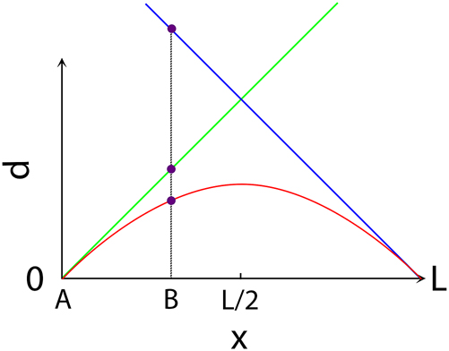
The plot of the three distances of the previous figure, as a function of the position x of the point B on the circle, the point A being fixed in the origin. The maximum value of the shortest one among the two Geodesic distances is L/2, while the maximum value of the Euclidean distance is L/π.

Once we have set the topology of the supercell and the Coulomb interaction between the particles, we need a wavefunction for the system. In the Quantum-Chemistry language, this means that we need the orbitals that describe the electrons. In the “Linear Combination of Atomic Orbitals” (LCAO) scheme, the Molecular Orbitals (MO) of the system are obtained as linear combinations of the Atomic Orbitals (AO) of the atoms. In the overwhelming majority of this type of calculations, the AO of the system are linear combinations of Gaussian functions, originally proposed by Boys as suitable functions to describe AOs. ³¹ Unfortunately, ordinary Gaussians have a major problem if used on a Torus: they are defined on the whole space R n . In simple words, we can say that they “go out” of the torus. However, if the width of the Gaussian is narrow enough with respect to the system size (i.e., if αL ² ≫ 1), a Gaussian function peaked in the central part of the torus will have a negligible values “out of the torus”. Therefore, one can neglect the non-zero part of the Gaussian which is out of the torus, and use the one- and two-electron integrals computed in R n . With this approximation, and by using ordinary Gaussians of s type with “large” exponents (more precisely, α ≫ 1/L ²), we have been able to treat ensembles of electrons having different values of the density, ranging from the Fermi gas (high density), ²⁰ to the Wigner crystal (low density). ¹⁵ Nevertheless, this approximation is obviously not completely satisfactory on the formal side, since we place in T functions which are defined in R . Moreover, there is a second, more serious problem: the use of Gaussians having a higher-than-zero angular momentum (p, d, etc.) is almost always needed in order to treat the atoms in a real crystals. Unfortunately, the introduction of this type of functions poses additional formal difficulties, that we were not able to overcome. For this reason, it would be much better to use continuous and differentiable orbitals that are defined in the torus only. This can be achieved by using orbitals that are combinations of toroidal Gaussians (we called them Clifford Gaussians), as will be described in detail in one of the next sections.

In this article, the Clifford formalism (i.e., Clifford boundary conditions and Clifford Gaussians) is used in order to investigate the behavior of two simple, model systems:

1. One electron on a 1-Dimensional (1D) torus (actually, a ring).

2. two electrons on a 2-Dimensional (2D) or 3-Dimensional (3D) torus.

The first system is analytically solvable. In atomic units, the eigenvalues of the Hamiltonian are given by k 2 2 , with k ∈ N, for a ring of length 2π. The corresponding eigenvectors, on the other hand, are combinations of the sine and cosine periodic functions on the ring. It will be shown that the exact eigenvalues, and hence the eigenvectors, can be approximated very precisely by using a set of sufficiently distributed Clifford Gaussians. Since the eigenvectors of the Hamiltonian form a complete basis set, this fact suggests that the Clifford Gaussians could have the same property. The second system has been numerically studied in a previous work of our group, by using a large number of distributed s-type ordinary Gaussians. In the present work, we show that, by using two Clifford Gaussians only, the numerically “exact” result can be very well approximated for a large range of electron densities. In particular, at low densities, the two electrons localize themselves in antipodal regions of the torus, forming a Wigner molecule.

This article is organized as follows. In Section “The Clifford formalism” we describe the Clifford formalism for periodic extended systems. In Section “Gaussian orbitals on a torus: Clifford Gaussians” we define the Clifford Gaussians on a torus, and some of their properties are discussed. In Section “One electron on a ring: an analytically solvable model” we study 1D system composed of one electron confined on 1D Torus, which is nothing but a ring. In Section “Two electrons in square and cubic Clifford Tori” we study the case of two electrons on a square or cubic torus. In Section “Conclusions and future perspectives”, we draw some conclusions, and discuss the future perspectives of our work. Finally, in the Appendix we prove the product theorem between two Clifford Gaussians, which is similar to the corresponding property holding for ordinary Gaussian functions.

The Clifford formalism

In the last few years, we have been developing an original formalism for the treatment of extended systems. The aim of the proposed formalism is to study a periodic infinite system by considering it as a large molecule, to which the standard ab initio methods of Quantum Chemistry can be applied. To this purpose, the following procedure is set up:

1. Extract a fragment (we call it a supercell, of the type discussed later) out of the infinite system, and give to the supercell the topology of a Clifford Torus. Then replace the ordinary geodesic distance that appears in the Coulomb interaction by a “renormalized” distance, given by the Euclidean distance in the complex space in which the Torus can be embedded.

2. Use periodic Gaussians, or “Clifford Gaussians”, possibly contracted ones, as the Atomic Orbitals of the system, compute the one- and two-electron integrals for these orbitals, and perform the desired ab initio calculation.

3. Repeat the two previous steps two by using toroidal supercells of similar shape but increasing sizes, in order to extrapolate the desired properties from finite oligomers to the infinite system at the thermodynamic limit.

As already anticipated, some caution must be used in the choice of the supercell. This must be a connected fragment of the whole system, composed of an integer number N of elementary unit cells, N = n ₁ ⋅ n ₂ ⋅ n ₃ in the 3D case, with similar expressions for the 1D and 2D crystals. Here n _i is an integer positive number that denotes the number of unit cells in the ith principal axis of the supercell. The extrapolation mentioned at the previous point 3. must be performed on supercells containing λn ₁ ⋅ λn ₂ ⋅ λn ₃ = λ ³ N unit cells, with λ a positive integer. Notice that the supercell λn ₁ ⋅ λn ₂ ⋅ λn ₃ becomes the whole system in the limit λ → ∞. At the moment, our formalism is able to treat right supercells only, whose shape is a rectangle in 2D and a right parallelepiped in 3D. Work is in progress to overcome this limitation.

We notice that, with respect to the ordinary molecular Quantum-Chemistry calculation, our approach for solids only requires rather limited modifications. The crucial advantage of our procedure is that these modifications only concern the calculation of the one- and two-electron integrals and the inter-nuclear repulsion, but are completely independent from the Quantum-Chemistry method used in the calculation. Therefore, once these modifications have been applied, any Quantum-Chemistry method (like Hartree–Fock (HF), Configuration Interaction (CI), Coupled Cluster (CC), Perturbation Theory (PT), etc.) can be used to perform calculations on periodic solids. Notice, however, that the use of Size-Consistent methods, like HF, CC or PT, is strongly recommended in order to extrapolate the results to the thermodynamic limit, step 3.

In summary, the proposed approach reduces the calculation of a solid to several calculations on Clifford supercells of increasing size. This is followed by the extrapolation to the thermodynamic limit. The smoothness and efficiency of the extrapolation are guaranteed by the topology of the Clifford Torus: the absence of boundaries, which eliminates border effects; and the zero Gaussian curvature, which insures that a crystal supercell can be fitted into the torus without any distortion. In a recent work, ²⁵ by using the example of ground-state energy of a chain of hydrogen atoms, we have shown that in the thermodynamic limit the results obtained within our approach are strictly equivalent to those obtained for a ring of the same atoms.

Gaussian orbitals on a torus: Clifford Gaussians

Generally speaking, a Gaussian Function g α , x 0 ( x ) can be defined in any metric space M , as

where x ₀ and x are two points that belong to M , while the exponent α is a real number. The point x ₀ is called the center of the Gaussian. Finally, d(x, x ₀) is the distance between x and x ₀ . If M is bounded, the exponent α can be any real number, otherwise it must be a strictly positive one, in order to insure that the Gaussian is a square-summable L ₂ function. If the distance d(x, x ₀) is a continuous (resp. differentiable) function between two points on M , the same property will hold for any Gaussian function defined on  M .

Equation (1) defines an unnormalized Gaussian. The corresponding normalized function, g ¯ α , x 0 ( x ) , is defined as

where N α , x 0 is a normalization constant given by N α , x 0 = 1 / C α , x 0 . Here the square norm C α , x 0 of the Gaussian g α , x 0 ( x ) is given by

In order to distinguish the Gaussian functions that are defined on different types of manifolds, we will use the notation R -Gaussians for functions defined on the whole real axes R , T -Gaussians if defined on a Torus T , S -Gaussians on a sphere S , and so on. Similar notations will be used in 2D and 3D manifolds. If not otherwise specified, with the simple term “Gaussian” we will refer to a R -Gaussian. All R -Gaussians have a similar shape, in the sense that they can be reduced to a unique function by a homothetic transformation of the x variable, associated to a redefinition of the exponent α: g λ 2 α ( x / λ ) = g α ( x ) , where, for the sake of simplicity, we considered the 1D case only, and we dropped the dependence on x ₀ by setting x ₀ = 0. For T -Gaussians, on the other hand, the situation is more complicated, since they depend on the two parameters α and L. (This is also true for S -Gaussians, but we will not consider here this type of functions). Notice that, unlike R -Gaussians, in the case of T -Gaussians the parameter α can assume also the value zero, in which case the Gaussian is a constant. Indeed, a constant is an L ²-summable function on T , but not on R . Strictly speaking, the same thing is true for negative values of α, although this type of functions do not have sofar any interest in Quantum Chemistry. In Fig. 3, we compare ordinary R -Gaussians, g _r , and Clifford T -Gaussians, g _c for three different values of α, and L = 2π: α = 0.5 (Fig. 3a), α = 1.0 (Fig. 3b), α = 2.0 (Fig. 3c). It appears that T -Gaussians are smooth and periodic in the interval [−π, π], contrary to R -Gaussians. Moreover, the difference between the two types of functions vanishes if the value of α increases. In Fig. 4, and with the same value L = 2π, the difference between the two types of Gaussians in reported: in Fig. 4a for α = 0.5, 1.0, 2.0, and 4.0; in Fig. 4b the difference times α, for α = 1.0, 10, 100, and 1000. It appears that the convergence to zero is relatively slow, particularly in the region of the inflection points of the curves, where there is a sort of spike whose height goes to zero as 1/α. This fact is put in evidence in particular in Fig. 4b.

Fig. 3:

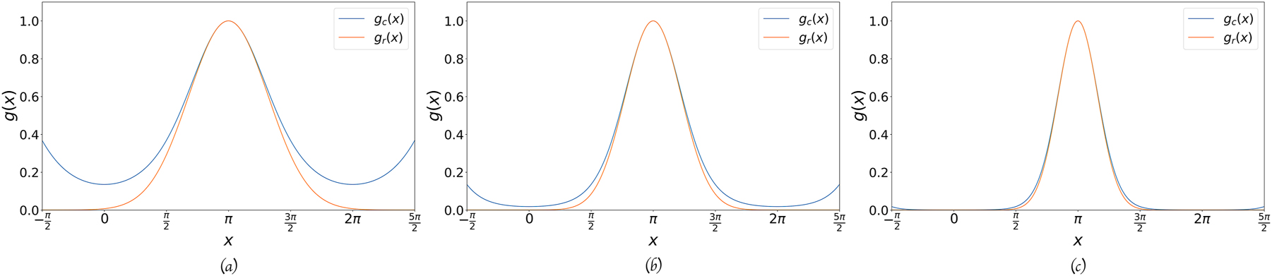
Comparison between the usual R -Gaussians, g _r and Clifford T -Gaussians, g _c for different values of the exponent. The center of all the Gaussians is in x = 0. (a) The two functions for α = 0.5. (b) The two functions for α = 1.0. (c) The two functions for α = 2.0.

Fig. 4:

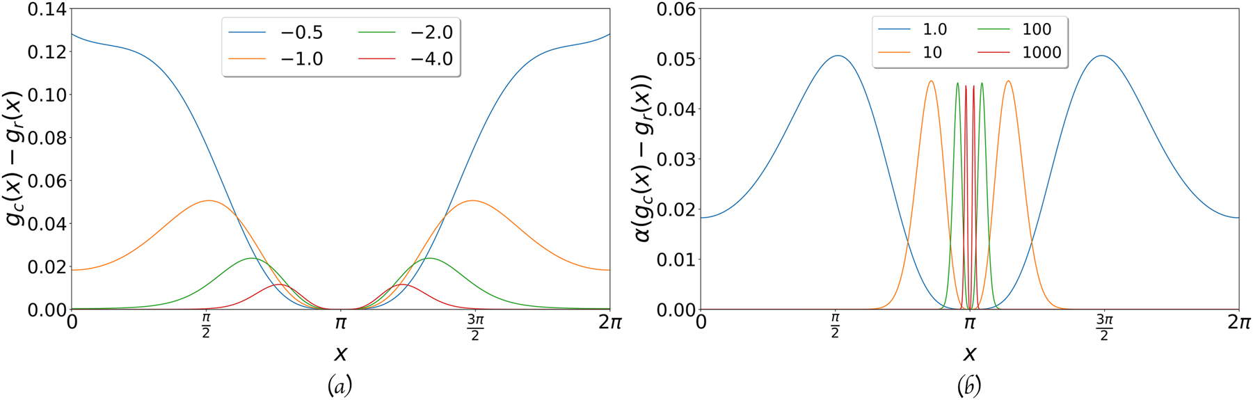
The difference between the two types of Gaussians for different values of the exponent. The center is in x = π. (a) The difference between the two functions, for α equal to 0.5, 1.0, 2.0, and 4.0. (b) The difference between the two functions times α, for α equal 1.0, 10.0, 100.0, and 1000.0.

The most common example of Atomic Orbitals is given by the Gaussian Atomic Orbitals, introduced by Boys in order to perform Molecular-Orbital calculations of atoms, molecules and periodic systems. ³¹ Today, the large majority of Quantum-Chemistry calculations is indeed performed within this type of orbitals. An s-type Gaussian Orbital is given, in 1D, by the function

where N _α is a normalization constant. The exponent α determines the Gaussian width. In fact, the two inflection points of the curve are located at positions satisfying | x 0 − x | = 1 / ( 2 α ) , which means that the Gaussian width is proportional to 1 / α . When a smooth function is approximated through a set of identical and evenly spaced Gaussians (as it was the case, for instance, for our studies on Wigner Crystals ^{15 , 20 , 24} ), a quantity that plays a crucial role is given by the dimensionless parameter ξ = αd ², where d is the distance between two neighboring Gaussians. For instance, if ξ > 2 the sum of two Gaussians is a double-peak function, while for ξ < 2 there is a single peak. Therefore, it appears to be problematic to approximate, say, a constant by using functions having a large value of ξ. (See our results on one electron in a ring in this article). A value of ξ much smaller than one, on the other hand, has the drawback of yielding numerical problems due to the quasi linear dependence of the orbitals. Moreover, from a practical point of view, smaller values of ξ require a larger number of function to pave the space. In our numerical experience with R -Gaussian functions, we found that a value of ξ = 1 is an upper bound in order to have stable results, and we often used ξ = 1 or ξ = 0.8.

It is possible to define Gaussian functions on other types of manifolds. For instance, Spherical-Gaussian Orbitals have been recently introduced by Loos, Gill and coworkers in order to describe the behavior of electrons on a 2D or 3D sphere. ^{32 , 33 , 34 , 35} On a Clifford Torus, continuous and derivable Gaussian Orbitals can be defined by using the Euclidean distance. For a Torus T of length L _x , in one dimension one has

where x ₀ is the center of the Gaussian, x ₀ ∈ [0, L _x ]. In a similar way, in two dimensions one can define Clifford Gaussians as the product of two 1D Gaussians,

and, in three dimensions, one has

In principle, it is possible to have different exponential parameters for the different space directions, α _x , α _y , and α _z . However, we will not take the opportunity of this freedom. Notice that Gaussian functions on the torus defined by using the Riemannian distance are continuous but not differentiable functions of the point positions, x and x ₀. On the other hand, the Clifford Gaussians that will be considered in the article are defined by using the Euclidean distance, and they are C ∞ functions of the two positions.

In actual calculations on atomic systems, Gaussians functions of higher angular momentum, p, d, f, and so on, are also considered, in order to describe the shell structure of the atoms. This definition can be extended to Clifford Gaussians, by replacing the function x and its powers in the polynomial part of orbital by the corresponding powers of L x 2 π sin ( 2 π x L x ) , with a similar procedure for y and z, and for the mixed products. In this paper, however, we will limit ourselves to s-type Gaussians only. A key property of R -Gaussians is their factorization property: the product of two Gaussians is a third Gaussian located in the exponent-barycenter of the two functions, x _c = (α ₁ x ₁ + α ₂ x ₂)/(α ₁ + α ₂), and with exponent given by α _c = (α ₁ α ₂)/(α ₁ + α ₂). In the case of T -Gaussians, we have a similar property, that can be stated, in the 1D case, in the following way: Given two 1D T -Gaussians of type s, having exponents equal to α ₁ and α ₂, and centered in the points x ₁ and x ₂ of a torus of length L _x , their product is a third Gaussian, multiplied by a suitable scale factor:

where

and

while C α 1 , α 2 , x 1 , x 2 , L x is a suitable constant (see Appendix for details). The generalization to the 2D and 3D cases is straightforward. This property of T -Gaussians will be proved in the Appendix. In the Fig. 5 we show the behavior of x _c and α _c for two Gaussians defined on a torus of length 2π for different values of α. The behavior depends essentially on the ratio between the exponents and it is symmetric under their permutation. For this reason, it is enough to fix the first exponent at α ₁ = 1, and explore the values 0 ≤ α ₂ ≤ 1 for the second one. The first center x ₁ is fixed in 0 and the position of the second one goes from 0 to 2π. For small values of x ₂, (i.e., for |x ₂|≪ 2π), the position x _c (Fig. 5a) and exponent α _c (Fig. 5b) are very much similar to the corresponding values for R -Gaussians. In particular, for α ₂ = α ₁, x _c is located in the middle point of the shortest arc that joins x ₁ and x ₂. This causes the discontinuity in the position of x _c at x ₂ = π, value for which the value of x _c is not defined. This discontinuity, however, has no consequences on the regularity of the results, since in this case we have that α _c  = 0, and the Gaussian is a constant. The exponent α _c of the product Gaussian, on the other hand, is comprised between the sum (when the two centers coincide) and the difference (when they are antipodean) of the two Gaussian exponents: |α ₁ − α ₂| < α _c  < α ₁ + α ₂.

Fig. 5:

The center and exponent of the Gaussian product of two Clifford T -Gaussians. The first Gaussian has α = 1 and center in x = 0, and the second one, with variable α, is centered in x ∈ [0, 2π]. The four curves correspond to the value of the second exponent of 1.0, 0.99; 0.9, 0.1. (a) The center x _c . (b) The exponent α _c .

The factorization property of the R -Gaussians that are used in ordinary Quantum-Chemistry calculations on isolated molecules has the advantage of a huge reduction of the numerical complexity in the evaluation of the required one- and two-electron integrals. ³⁶ In exactly the same way, we can use the factorization property of T -Gaussians in order to simplify the huge number of multicenter integrations that are needed among the orbitals in the supercell.

One electron on a ring: an analytically solvable model

The model of an electron freely moving in a 1D Torus (or equivalently, a ring) is exactly solvable with an analytic approach. It is essentially coincident with the well known rigid-rotator system. For the sake of simplicity, and since the physics of the system do not depend on the size of the ring, we consider an electron confined on a ring of length 2π. In atomic units, the energy levels of the system are given by the expression

Therefore, all the energy levels are positive and doubly degenerate, except for the ground-state one, E ₀ = 0. We describe the system through a set of N equally spaced 1D Clifford Gaussians, having a common exponent α. The spacing d between two neighboring Gaussians is therefore 2π/N. In our previous investigations by using ordinary Gaussians, we found that a crucial parameter that must be considered is the quantity ξ = αd ², as we already mentioned in a previous Section. Indeed, if ξ is significantly lower than one, the system of Gaussians becomes almost linearly dependent. On the other hand, if ξ is much greater than one, the Gaussians are very sharp, and therefore are not able to describe a smooth function.

We computed the overlap and kinetic matrix elements on this basis set, and diagonalized the resulting Hamiltonian. The resulting approximated eigenvalues are denoted as E ¯ k , with k = 0, …, N − 1. In order to assess the capability of the Clifford-Gaussian functions to span the space of the eigenvalues of the Hamiltonian, we computed, for any given value of α, the quantity

which is the mean quadratic deviation of the first N/2 approximate eigenvalues with respect to the exact ones. Notice that in the last equation the notations for the exact eigenvalues in eqs. (12) and (13) are slightly different, and no negative labels are considered for the approximate eigenvalues.

In Table 1, we report the results obtained for different values of N, and, for each value of N, for a set of different values of α. In order to simplify the comparison between the different cases, both N and α have been chosen as powers of two. However, a finer sampling of α could have been explored in order to better minimize Δ. For each value of N and α, we report in the table the value of ξ = α d ², the lowest eigenvalue of the overlap, S ₀, and the mean quadratic error Δ N α . It turns out that two neighboring Gaussians must have a noticeable overlap in order to allow the basis set to efficiently reproduce the N/2 lowest eigenvalues. Indeed, when ξ > 1, the quality of the result quickly deteriorates. This is well illustrated in the case N = 16, for which we explored a rather large set of values of α. On the other hand, it is always possible to find a range of α values that permit an accurate description of the lowest N/2 eigenvalues, even when N is relatively large. These results seem to indicate that the Clifford Gaussians could form a basis set asymptotically complete, provided the value of ξ is kept sufficiently small while the number of functions is increased. We are currently working on this important aspect of the formalism, both on the formal mathematical side and the numerical results.

Two electrons in square and cubic Clifford Tori

In this section, we use the Clifford formalism to describe the behavior of two electrons confined into a torus. The strictly 1D system is ill defined, because of the singularity of the 1D Coulomb potential at short range. Therefore, we limit our investigation to the 2D and 3D cases. In both the 2D and 3D cases, a single Clifford Gaussian is enough to describe one unpaired electron, so a total of two orbitals for the entire system is qualitatively enough.

Results

We considered several square and cubic Tori of different size, going from relatively high electron density (L = 1 bohr) to very low density (L = 10⁶ bohr). Notice that with two electrons only and periodic boundary conditions, the high-density limit of the kinetic energy is zero, and one doubly occupied constant orbital minimizes the total energy. Therefore, the high-density limit is not particularly interesting, and we did not explore values of α lower than one. In each case, by spanning a large range of values of the exponent α, we performed the Self-Consistent Field (SCF) and Full Configuration Interaction (FCI) calculations. In order to do this, we numerically computed the 1-e and 2-e integrals, as discussed in ref. 25]. Then, for each value of the Torus size L, we computed the values of the exponents α that minimize the SCF and FCI energies for the ground ¹Σ _g state, in order to find the best two-orbital wavefunction that describes the system at these two levels.

The FCI wave-function

Things are much more interesting at FCI level. In this case, due to the Coulomb repulsion, the two electrons tend to localize at opposite positions in the Torus. Therefore, we restricted our investigation to this position of the orbitals. As discussed in a previous article, ¹⁵ the shape of the wavefunction is the result of two different, competing, phenomena. The kinetic energy tends to distribute the electrons as much as possible, and reaches its minimum (T _min = 0) for a constant orbital. The electron-electron repulsion, on the other hand, reaches its minimum for two delta-like orbitals located as far apart as possible one from the other one in the Torus. In this case we have V min = π / L n (here n is the number of space dimensions, in the present case n = 2 or n = 3). It is the balance between these two opposite effects that gives the actual shape of the system orbitals. The kinetic energy dominates at high density, while the Coulomb repulsion is the main effect at low density, even though both terms vanish in this limit.

The results for several values of L are reported in Table 2. For each L, the value of α which minimizes the ground-state ¹Σ _g energy is numerically obtained. At large values of L, the electrons are completely localized in one orbital, and the wave-function is totally neutral in the Valence-Bond language. In this case, the singlet and triplet lowest states, Σ g 1 = 1 2 ( g 1 g ¯ 2 + g 2 g ¯ 1 ) and ³ Σ u = 1 2 ( g 1 g ¯ 2 − g 2 g ¯ 1 ) become degenerate. The antisymmetric singlet, on the other hand, is much higher in energy, due to its ionic nature, since in term of local orbitals it is given by ¹ Σ u = 1 2 ( g 1 g ¯ 1 − g 2 g ¯ 2 ) . Notice, however, that this effect is enhanced by the value of the exponent α, which has been optimized for the neutral ground-state singlet. In the Fig. 6, we report the optimum-α orbitals for the square (Fig. 6a) and the cubic (Fig. 6b) tori. The three values L = 10, L = 10³, and L = 10⁵ have been reported in each figure. Notice that the electrons at L = 10 are already rather delocalized in the whole torus, since the Gaussians are very flat.

Table 2:

The FCI energies (Hartree) of the different states as a function of the system size L, in Bohr, for the square T 2 (top) and cubic T 3 tori (bottom). The energies are multiplied by L in order to facilitate the comparison. E _FCI (N*Gauss) is the reference energy, from ref. 15], obtained by using 40 ⋅ 40 and 10 ⋅ 10 ⋅ 10 Gaussians, respectively, and ξ = 1. The exponent α is the optimum value of the exponent that minimizes the energy of the singlet ¹Σ _g ground state by using two Clifford Gaussians (this work); then for this value of α, the FCI energies of the three low-lying states, multiplied by L, are reported.

L	E FCI (N*Gauss) ⋅ L	α	E(1Σ g ) ⋅ L	E(3Σ u ) ⋅ L	E(1Σ u ) ⋅ L
1	3.830402736	0.6482352941	4.013014260	22.748626240	24.8102329
10	3.341151624	0.0551427593	3.806440756	4.956076291	7.21759770
100	2.696524187	0.0024538105	2.940311452	2.937831178	8.46944608
1000	2.367285277	0.0000614009	2.436287842	2.436287795	13.6487884
10 000	2.264144855	0.0000017332	2.288165632	2.288165632	23.1742091
100 000	2.231970680	0.0000007700	2.244004858	2.244004858	49.3331443
1 000 000	2.221862760	0.0000000190	2.222820000	2.222820000	78.8513000
1	2.872009610	0.1962500180	2.857732292	22.239451744	22.961051
10	2.652234404	0.0186927727	2.829355521	4.470156885	5.206218
100	2.248181503	0.0015801231	2.543355955	2.553775202	4.430400
1000	1.921838799	0.0000107829	2.034108452	2.034108453	11.905348
10 000	1.810452655	0.0000012884	1.887462369	1.887462369	12.727726
100 000	/	0.0000000662	1.829425683	1.829425683	39.288272
1 000 000	/	0.0000000041	1.817885691	1.817885691	52.637321

Fig. 6:

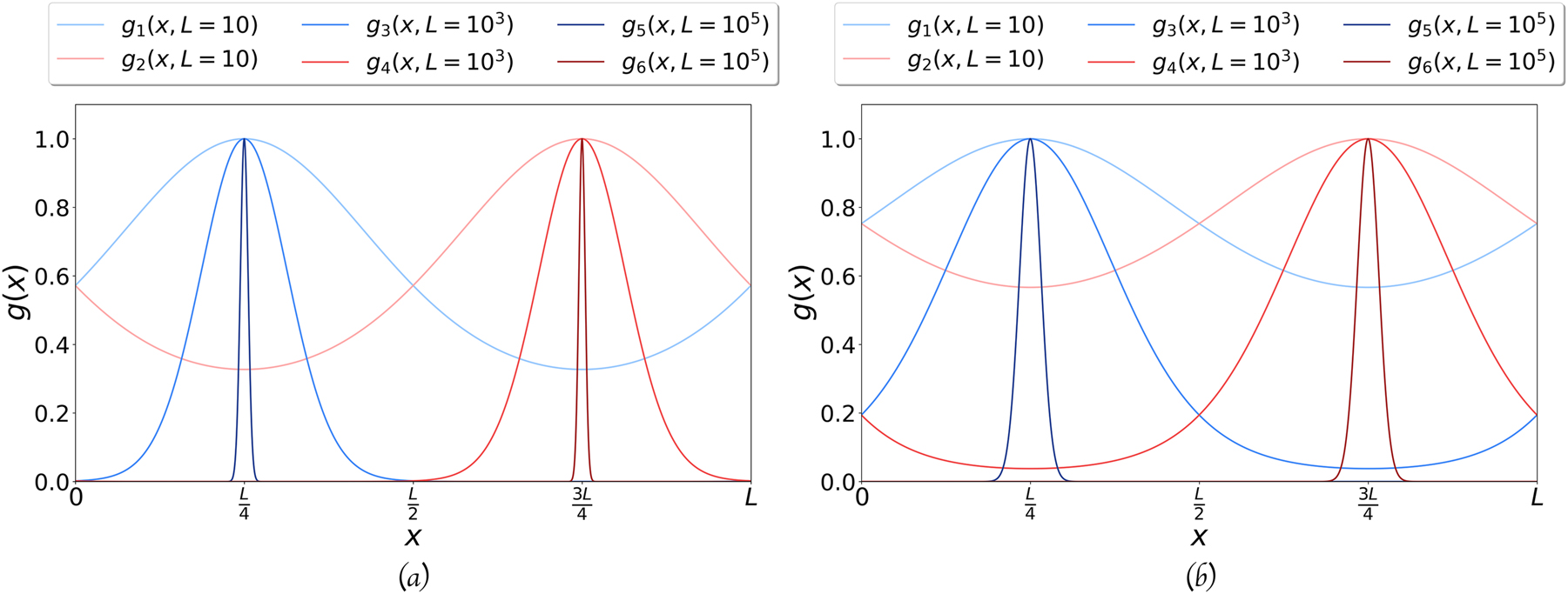
Comparison of the shape of the optimal Gaussians for different values of the side L. (a) The two Gaussian orbitals on the square: optimum value of α, for the square side L equal to 10 (g ₁, g ₂), 1000 (g ₃, g ₄), and 100 000 (g ₅, g ₆). A factor 2 is implicit and not shown in the x axis. (b) The two Gaussian orbitals on the cube: optimum value of α, for the cube side L equal to 10 (g ₁, g ₂), 1000 (g ₃, g ₄), and 100 000 (g ₅, g ₆). A factor 3 is implicit and not shown in the x axis.

It is interesting to compare these results, obtained by using a pair of Clifford Gaussians only, with the corresponding values from reference, for which the FCI energies by using a relatively large number of ordinary Gaussians were computed. ¹⁵ The present energy values are only a few percent higher than the FCI “exact” results for intermediate values of the density, probably because of dynamical-correlation effects, and only a fraction of percent at very low densities. This confirms the well known fact that the orbitals of the electrons in a Wigner Crystal have a Gaussian shape. ³⁷ More importantly, since a small number of orbitals per electron is required to describe the system (just one, or a few ones if the effects of correlation are to be taken into account), this could open the way to a full quantum treatment of Wigner Crystals by using the methods of Quantum Chemistry.

Conclusions and future perspectives

We presented a general paradigm for the treatment of infinite periodic systems within the framework of Quantum Chemistry. Our approach is based on three main steps.

1. Associate the topology of a Clifford Torus to a supercell of the system, and choose the Euclidean distance in the torus as the distance that appears in the Coulomb interaction, and, more generally, in any distance-dependent property of the system.

2. Define the AOs of the system as a combination of Clifford Gaussians in the torus, and build the MOs from this set of AOs; use your favorite Quantum Chemistry method (if possible, a size-consistent one) to investigate the system.

3. Repeat this procedure for a set of supercells of increasing size and similar shape, in order to extrapolate the desired properties of the system to the infinite thermodynamical limit.

In the present work, in particular, we numerically investigated two important model systems: one particle in a box (a 1D system), and two electrons confined in a Clifford Torus (2D and 3D).

1. In the first case, we showed that a set of N Clifford Gaussians having a suitable exponent is able to reproduce the lowest N/2 eigenvalues of the Hamiltonian to an extremely high accuracy, comparable with the machine precision of the computer (all the calculations have been done in double precision). This fact strongly suggests that these functions could form, under certain circumstances, a complete basis set for the one-particle Hilbert Space that is used in Quantum Mechanics.

2. The second case is particularly pertinent for the description of free electrons at very low density, a situation that gives rise to the so called Wigner Localization. Our investigation shows that one single Clifford Gaussian per electron is able to qualitatively describe the localization of the electrons. By comparison, a large number of R -Gaussians had to be employed in order to obtain numerically converged results on this system.

We are presently working on a mathematical proof of the completeness property of Clifford Gaussians for one-particle systems, that at the moment we have only guessed. The treatment of systems composed of a large number of free electrons by using this type of Gaussians, in order to investigate the behavior of Wigner Crystals, is also being considered.

Our investigation is certainly preliminary, and we are currently working to the application of our scheme to realistic systems. We think, in particular, to real 2D and 3D systems, like graphene, diamond, ionic crystals, and so on. Also rigid quasi-1D systems, that cannot be treated by arranging the atoms on a circle, like Carbon or Boron-Nitride nanotubes, would be particularly suitable for our approach. The treatment of such systems would require the introduction of high angular-momentum orbitals in the atomic basis set. At the moment, we are testing the calculation of the two-electron integrals for p functions, and implementing the integrals for d orbitals. Preliminary tests indicate that the computer time required to obtain the integrals over Clifford Gaussians is comparable to the same time needed in the case of ordinary Gaussians. This is a very encouraging result, also considering the rather preliminary state of our investigation. If these results will be confirmed by further investigations, we believe that our approach could open the road to an ab initio treatment of periodic systems, in the same way as molecules and clusters are presently treated by Quantum Chemistry.

References

1. Sun, J.-Q.; Bartlett, R. J. Second-Order Many-Body Perturbation-Theory Calculations in Extended Systems. J. Chem. Phys. 1996, 104, 8553–8565; https://doi.org/10.1063/1.471545.Search in Google Scholar
2. Ayala, P. Y.; Kudin, K. N.; Scuseria, G. E. Atomic Orbital Laplace-Transformed Second-Order Møller–Plesset Theory for Periodic Systems. J. Chem. Phys. 2001, 115, 9698–9707; https://doi.org/10.1063/1.1414369.Search in Google Scholar
3. Hirata, S.; Podeszwa, R.; Tobita, M.; Bartlett, R. J. Coupled-Cluster Singles and Doubles for Extended Systems. J. Chem. Phys. 2004, 120, 2581–2592; https://doi.org/10.1063/1.1637577.Search in Google Scholar PubMed
4. Pisani, C.; Busso, M.; Capecchi, G.; Casassa, S.; Dovesi, R.; Maschio, L.; Zicovich-Wilson, C.; Schütz, M. Local-MP2 Electron Correlation Method for Nonconducting Crystals. J. Chem. Phys. 2005, 122, 094113; https://doi.org/10.1063/1.1857479.Search in Google Scholar PubMed
5. Katagiri, H. Equation-Of-Motion Coupled-Cluster Study on Exciton States of Polyethylene with Periodic Boundary Condition. J. Chem. Phys. 2005, 122, 224901; https://doi.org/10.1063/1.1929731.Search in Google Scholar PubMed
6. Marsman, M.; Grüneis, A.; Paier, J.; Kresse, G. Second-Order Møller–Plesset Perturbation Theory Applied to Extended Systems. I. Within the Projector-Augmented-Wave Formalism Using a Plane Wave Basis Set. J. Chem. Phys. 2009, 130, 184103; https://doi.org/10.1063/1.3126249.Search in Google Scholar PubMed
7. Grüneis, A.; Booth, G. H.; Marsman, M.; Spencer, J.; Alavi, A.; Kresse, G. Natural Orbitals for Wave Function Based Correlated Calculations Using a Plane Wave Basis Set. J. Chem. Theory Comput. 2011, 7, 2780–2785; https://doi.org/10.1021/ct200263g.Search in Google Scholar PubMed
8. Pisani, C.; Schütz, M.; Casassa, S.; Usvyat, D.; Maschio, L.; Lorenz, M.; Erba, A. Cryscor: A Program for the Post-Hartree–Fock Treatment of Periodic Systems. Phys. Chem. Chem. Phys. 2012, 14, 7615; https://doi.org/10.1039/c2cp23927b.Search in Google Scholar PubMed
9. Shepherd, J. J.; Grüneis, A.; Booth, G. H.; Kresse, G.; Alavi, A. Convergence of Many-Body Wave-Function Expansions Using a Plane-Wave Basis: From Homogeneous Electron Gas to Solid State Systems. Phys. Rev. B 2012, 86, 035111; https://doi.org/10.1103/physrevb.86.035111.Search in Google Scholar
10. Booth, G. H.; Grüneis, A.; Kresse, G.; Alavi, A. Towards an Exact Description of Electronic Wavefunctions in Real Solids. Nature 2013, 493, 365–370; https://doi.org/10.1038/nature11770.Search in Google Scholar PubMed
11. McClain, J.; Sun, Q.; Chan, G. K.-L.; Berkelbach, T. C. Gaussian-Based Coupled-Cluster Theory for the Ground-State and Band Structure of Solids. J. Chem. Theory Comput. 2017, 13, 1209–1218; https://doi.org/10.1021/acs.jctc.7b00049.Search in Google Scholar PubMed
12. Wang, X.; Berkelbach, T. C. Excitons in Solids from Periodic Equation-of-Motion Coupled-Cluster Theory. J. Chem. Theory Comput. 2020, 16, 3095–3103; https://doi.org/10.1021/acs.jctc.0c00101.Search in Google Scholar PubMed
13. Erba, A.; Desmarais, J. K.; Casassa, S.; Civalleri, B.; Donà, L.; Bush, I. J.; Searle, B.; Maschio, L.; Edith-Daga, L.; Cossard, A.; Ribaldone, C.; Ascrizzi, E.; Marana, N. L.; Flament, J.-P.; Kirtman, B. CRYSTAL23: A Program for Computational Solid State Physics and Chemistry. J. Chem. Theory Comput. 2023, 19, 6891–6932; https://doi.org/10.1021/acs.jctc.2c00958.Search in Google Scholar PubMed PubMed Central
14. Valença Ferreira de Aragão, E.; Moreno, D.; Battaglia, S.; Bendazzoli, G. L.; Evangelisti, S.; Leininger, T.; Suaud, N.; Berger, J. A. A Simple Position Operator for Periodic Systems. Phys. Rev. B 2019, 99, 205144; https://doi.org/10.1103/physrevb.99.205144.Search in Google Scholar
15. Escobar Azor, M.; Brooke, L.; Evangelisti, S.; Leininger, T.; Loos, P.-F.; Suaud, N.; Berger, A. A Wigner Molecule at Extremely Low Densities: A Numerically Exact Study. SciPost Phys. Core 2019, 1, 001; https://doi.org/10.21468/scipostphyscore.1.1.001.Search in Google Scholar
16. Tavernier, N.; Bendazzoli, G. L.; Brumas, V.; Evangelisti, S.; Berger, J. A. Clifford Boundary Conditions: A Simple Direct-Sum Evaluation of Madelung Constants. J. Phys. Chem. Lett. 2020, 11, 7090–7095; https://doi.org/10.1021/acs.jpclett.0c01684.Search in Google Scholar PubMed
17. Tavernier, N.; Bendazzoli, G. L.; Brumas, V.; Evangelisti, S.; Berger, J. A. Clifford Boundary Conditions for Periodic Systems: The Madelung Constant of Cubic Crystals in 1, 2 and 3 Dimensions. Theor. Chem. Acc. 2021, 140, 106; https://doi.org/10.1007/s00214-021-02805-1.Search in Google Scholar
18. Alves, E.; Bendazzoli, G. L.; Evangelisti, S.; Berger, J. A. Accurate Ground-State Energies of Wigner Crystals from a Simple Real-Space Approach. Phys. Rev. B 2021, 103, 245125; https://doi.org/10.1103/physrevb.103.245125.Search in Google Scholar
19. Angeli, C.; Bendazzoli, G. L.; Evangelisti, S.; Berger, J. A. The Localization Spread and Polarizability of Rings and Periodic Chains. J. Chem. Phys. 2021, 155, 124107; https://doi.org/10.1063/5.0056226.Search in Google Scholar PubMed
20. Escobar Azor, M.; Alves, E.; Evangelisti, S.; Berger, J. A. Wigner Localization in Two and Three Dimensions: An Ab Initio Approach. J. Chem. Phys. 2021, 155, 124114; https://doi.org/10.1063/5.0063100.Search in Google Scholar PubMed
21. Evangelisti, S.; Abu-Shoga, F.; Angeli, C.; Bendazzoli, G. L.; Berger, J. A. Unique One-Body Position Operator for Periodic Systems. Phys. Rev. B 2022, 105, 235201; https://doi.org/10.1103/physrevb.105.235201.Search in Google Scholar
22. François, G.; Angeli, C.; Bendazzoli, G. L.; Brumas, V.; Evangelisti, S.; Berger, J. A. Mapping of Hückel Zigzag Carbon Nanotubes onto Independent Polyene Chains: Application to Periodic Nanotubes. J. Chem. Phys. 2023, 159, 094106; https://doi.org/10.1063/5.0153075.Search in Google Scholar
23. Alrakik, A.; Escobar Azor, M.; Brumas, V.; Bendazzoli, G. L.; Evangelisti, S.; Berger, J. A. Solution to the Thomson Problem for Clifford Tori with an Application to Wigner Crystals. J. Chem. Theory Comput. 2023, 19, 7423–7431; https://doi.org/10.1021/acs.jctc.3c00550.Search in Google Scholar
24. Escobar Azor, M.; Alrakik, A.; De Bentzmann, L.; Telleria-Allika, X.; Sánchez de Merás, A.; Evangelisti, S.; Berger, J. A. The Emergence of the Hexagonal Lattice in Two-Dimensional Wigner Fragments. J. Phys. Chem. Lett. 2024, 15, 3571–3575; https://doi.org/10.1021/acs.jpclett.4c00453.Search in Google Scholar
25. Alrakik, A.; Bendazzoli, G. L.; Evangelisti, S.; Berger, J. A. Quantum Chemistry for Solids Made Simple with the Clifford Formalism, 2025. Available from: https://arxiv.org/abs/2508.03917.Search in Google Scholar
26. Noga, J.; Baňack, P.; Biskupič, S.; Boča, R.; Pelikán, P.; Svrčeký, M.; Zajac, A. Approaching Bulk Limit for Three-Dimensional Solids Via the Cyclic Cluster Approximation: Semiempirical INDO Study. J. Comput. Chem. 1999, 20, 253–261; https://doi.org/10.1002/(sici)1096-987x(19990130)20:2<253::aid-jcc7>3.0.co;2-9.10.1002/(SICI)1096-987X(19990130)20:2<253::AID-JCC7>3.0.CO;2-9Search in Google Scholar
27. Volkert, K. Space Forms: A History. Bull. Manifold Atlas 2013, 1–5.Search in Google Scholar
28. McIntosh, A.; Mitrea, M. Clifford Algebras and Maxwell’s Equations in Lipschitz Domains. Math. Methods Appl. Sci. 1999, 22, 1599–1620; https://doi.org/10.1002/(sici)1099-1476(199912)22:18<1599::aid-mma95>3.3.co;2-d.10.1002/(SICI)1099-1476(199912)22:18<1599::AID-MMA95>3.3.CO;2-DSearch in Google Scholar
29. Clifford. Preliminary Sketch of Biquaternions. Proc. Lond. Math. Soc. 1871 (s1–4), 381–395; https://doi.org/10.1112/plms/s1-4.1.381.Search in Google Scholar
30. Klein, F. Zur Nicht-Euklidischen Geometrie. Math. Ann. 1890, 37, 544–572; https://doi.org/10.1007/bf01724772.Search in Google Scholar
31. Boys, S. F. Electronic Wave Functions - I. A General Method of Calculation for the Stationary States of Any Molecular System. Proc. Roy. Soc. Lond. Ser. A. Math. Phys. Sci. 1950, 200, 542–554.10.1098/rspa.1950.0036Search in Google Scholar
32. Loos, P.-F.; Gill, P. M. W. Uniform Electron Gases. I. Electrons on a Ring. J. Chem. Phys. 2013, 138, 164124; https://doi.org/10.1063/1.4802589.Search in Google Scholar
33. Loos, P.-F.; Ball, C. J.; Gill, P. M. W. Uniform Electron Gases. II. the Generalized Local Density Approximation in One Dimension. J. Chem. Phys. 2014, 140, 18A524; https://doi.org/10.1063/1.4867910.Search in Google Scholar PubMed
34. Gill, P. M. W.; Loos, P.-F.; Agboola, D. Basis Functions for Electronic Structure Calculations on Spheres. J. Chem. Phys. 2014, 141, 244102; https://doi.org/10.1063/1.4903984.Search in Google Scholar PubMed
35. Agboola, D.; Knol, A. L.; Gill, P. M. W.; Loos, P.-F. Uniform Electron Gases. III. Low-density Gases on Three-Dimensional Spheres. J. Chem. Phys. 2015, 143, 084114; https://doi.org/10.1063/1.4929353.Search in Google Scholar PubMed
36. Szabo, A.; Ostlund, N. Modern Quantum Chemistry: Introduction to Advanced Electronic Structure Theory; Dover Books on Chemistry; Dover Publications: New York, USA, 1996.Search in Google Scholar
37. Giuliani, G.; Vignale, G. Quantum Theory of the Electron Liquid, 1st ed.; Cambridge University Press: Cambridge, UK, 2005.10.1017/CBO9780511619915Search in Google Scholar
© 2025 IUPAC & De Gruyter
Articles in the same Issue
- Frontmatter
- IUPAC Recommendations
- Experimental methods and data evaluation procedures for the determination of radical copolymerization reactivity ratios from composition data (IUPAC Recommendations 2025)
- IUPAC Technical Reports
- Kinetic parameters for thermal decomposition of commercially available dialkyldiazenes (IUPAC Technical Report)
- FAIRSpec-ready spectroscopic data collections – advice for researchers, authors, and data managers (IUPAC Technical Report)
- Review Articles
- Are the Lennard-Jones potential parameters endowed with transferability? Lessons learnt from noble gases
- Quantum mechanics and human dynamics
- Quantum chemistry and large systems – a personal perspective
- The organic chemist and the quantum through the prism of R. B. Woodward
- Relativistic quantum theory for atomic and molecular response properties
- A chemical perspective of the 100 years of quantum mechanics
- Methylene: a turning point in the history of quantum chemistry and an enduring paradigm
- Quantum chemistry – from the first steps to linear-scaling electronic structure methods
- Nonadiabatic molecular dynamics on quantum computers: challenges and opportunities
- Research Articles
- Alzheimer’s disease – because β-amyloid cannot distinguish neurons from bacteria: an in silico simulation study
- Molecular electrostatic potential as a guide to intermolecular interactions: challenge of nucleophilic interaction sites
- Photophysical properties of functionalized terphenyls and implications to photoredox catalysis
- Combining molecular fragmentation and machine learning for accurate prediction of adiabatic ionization potentials
- Thermodynamic and kinetic insights into B10H14 and B10H14 2−
- Quantum origin of atoms and molecules – role of electron dynamics and energy degeneracy in atomic reactivity and chemical bonding