Investigating the modified UO-iteration process in Banach spaces by a digraph
-
Esra Yolacan


Abstract
Graph theory (GT) is a highly captivating area of study within applied mathematics. Over the last 50 years, the number of mathematicians contributing to research in this field has consistently risen. This surge in interest can largely be attributed to its vast potential for practical applications. It has found uses in various disciplines such as engineering, physical sciences, genetics, computer science, sociology, operations research and economics. Driven and encouraged by these points, we introduce and analyze the convergence theorems for the modified UO-iterative sequences applied to
1 Introduction
Fixed point theory is a dynamic and rapidly developing area of research, primarily due to its broad applicability in many fields. It focuses on results that under specific conditions, a self-map on a set has at least one fixed point. The Banach contraction principle (BCP) [1] is arguably the most renowned result in metric fixed point theory, largely due to its straightforwardness and the convenience with which it can be applied in key areas of mathematics. Following that, the BCP has been generalized in a wide variety of ways. Jachymski [2] gave a new concept of
In [13], they study the following iterative sequence to approximate some fixed point of
Definition 1.1
Let
where
Building on the aforementioned work, we devised a modified UO-iteration process containing a
Definition 1.2
Let
where
If
The remainder of this article is structured as follows: Section 2 focuses on preliminary definitions and lemmas. Section 3 presents the convergence analysis of (1.2) for a
2 Preliminaries
In this section, we bring together some familiar concepts and relevant conclusions that will be frequently used.
Let
Definition 2.1
[2] A digraph
Definition 2.2
[5] A mapping
Definition 2.3
[8] Let
From this point on,
Definition 2.4
[14] A Banach space
Definition 2.5
[8] Let
Definition 2.6
[8] Let
Definition 2.7
[15] Let
Lemma 2.8
[16] Let
Lemma 2.9
[17] Let
imply that
Lemma 2.10
[18] Let
3 Main results
Unless specified differently, we will assume for the entirety of this part that
Proposition 3.1
Let
Proof
We carry on with induction. Considering
Due to edge-preserving of
As
By using edge-preserving of
Since
Continuing in this fashion for
Lemma 3.2
If L is a nonvoid closed convex subset of a real uniformly convex Banach space
Proof
(i) By Proposition 3.1,
and
By using Lemma 2.8, we have
(ii) Suppose that
In addition, from
As
Due to (3.9), (3.14), (3.15), and Lemma 2.9, we have
Moreover, we see that
By using (3.16) and (3.17), we obtain
so that (3.9) and (3.18), we obtain
Note that
Due to (3.8), (3.13), (3.20), and Lemma 2.9, we have
Further, we see that
such that (3.8) and (3.23) are satisfied, we obtain
Note that
Owing to (3.7), (3.12), (3.25), and Lemma 2.9, we have
Furthermore, we see that
and combining them with (3.7) and (3.28), we obtain
Note that
Owing to (3.6), (3.10), (3.30), and Lemma 2.9, we have
Moreover, we see that
such that (3.6) and (3.33) are satisfied, we obtain
Note that
Due to (3.11) and Lemma 2.9, we have
Proposition 3.3
Assume that
Proof
Suppose that
This is a contradiction. Therefore,
Theorem 3.4
Assume that
Proof
Let
Theorem 3.5
Assume that
Proof
By Lemma 3.2 (ii), we know
Here, at
4 Image deblurring
Image deblurring is a well-established challenge in low-level computer vision, which has drawn considerable interest from both the image processing and computer vision fields. The goal of image deblurring is to restore a clear image from a blurred input, with the blur often resulting from factors such as insufficient focus, camera shake, or rapid motion of the subject [19–21]. Image deblurring often relies on iterative algorithms as a standard approach. On the basis of these insights, we devised an iterative technique to deblur (sharpen) a blurred image by combining the powerful scientific computing and graphics capabilities in Matlab R2016a.
We shall now describe the operations carried out in the developed code, systematically presenting the sequence of steps to illustrate the order of execution:
Step 1: Retrieving and Preparing the Image.
Step 2: Modeling Motion.
Step 3: Setting Novel Iteration Parameters.
Step 4: Implementing Iterative Refinements.
Step 5: Displaying the Results.
This code is designed to iteratively restore a blurred image. A blurred image is first generated, and then an iterative process using inverse filtering is employed to progressively improve the estimation of the sharp image. The results are visualized at regular intervals (every 10 iterations) to observe the advancement of the deblurring process. The images reconstructed with the recommended algorithm at the 10th, 20th, 30th, 40th, and 50th iterations are shown using the subplot command, which visually presents the results at every 10th iteration. The original image, the blurred image, and the deblurred image (obtained after 50 iterations) are presented together as shown in Figure 1.
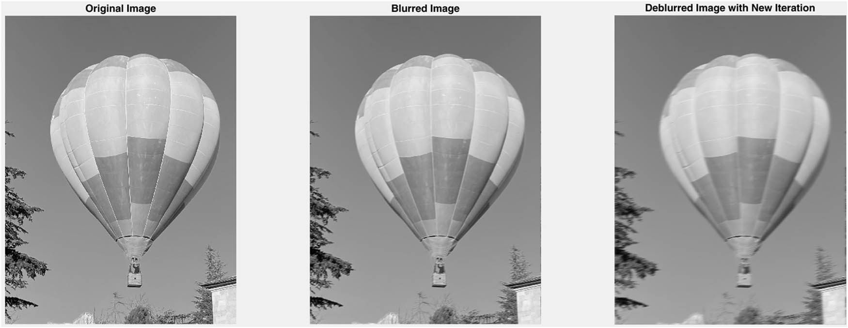
The original image, the blurred image, and the deblurred image.
This allows for monitoring the evolution of the deblurring process. Balloon fig displays a side-by-side comparison of the original image, the blurred image, and the deblurred image after 50 iterations. The visualization highlights the difference between the original and blurred images, as well as the improvements made by the 50th iteration in the deblurring process.
In conclusion, while these algorithms are applicable in various fields, more complex blur types may require the incorporation of additional strategies and careful parameter adjustment to achieve optimal results. By revising the code and fine-tuning the parameters, the accuracy of the output can be improved.
Example 4.1
The value of each pixel in the original image (that is, balloon) is actually a number (between 0 and 1, grayscale). Patch
Notice that each pixel value is given as 0.4745. This means that all pixels in a grayscale image have the same intensity. Now, let me explain step by step how to run the proposed algorithm (iterative deblurring) on this patch:
Step 1: Getting the Patch Matrix.
Step 2: Motion Blur (Point Spread Function) Definition.
Step 3: Creating Blurred Image
As a result, the initial patch and the blurred image were the same because all pixels in the patch already had the same value. That is, the blurring effect was not very noticeable.
Step 4: Iterative Deblurring Algorithm.
Step 5: Deblurring Process (Iterations).
Consequently, the patch we first supplied was a
5 Signal enhancement
Signal enhancement is a technique used to reduce noise, thereby improving the signal’s clarity and increasing the proportion of the desired signal relative to the noise [22]. This technique is essential in various engineering fields, particularly in areas like image analysis, audio processing, medical imaging, and telecommunications [23]. To address intricate signal enhancement issues, iterative methods are frequently employed [24]. These methods are important for refining procedures and increasing the precision of the results in signal enhancement [25]. Drawing from these ideas, we created a code that generates a noisy signal based on a sine wave, utilizes an iterative algorithm to refine the signal, and visualizes the original, noisy, and enhanced signals in Matlab R2016a. Below is a comprehensive step-by-step explanation of this code:
Step 1: Producing the Original Signal (Clean Sine Wave) and the Noisy Signal (Sine Wave With Gaussian Noise introduced).
Step 2: Developing a New Iterative Signal Improvement Algorithm.
Step 3: Plotting the Results.
In this regard,
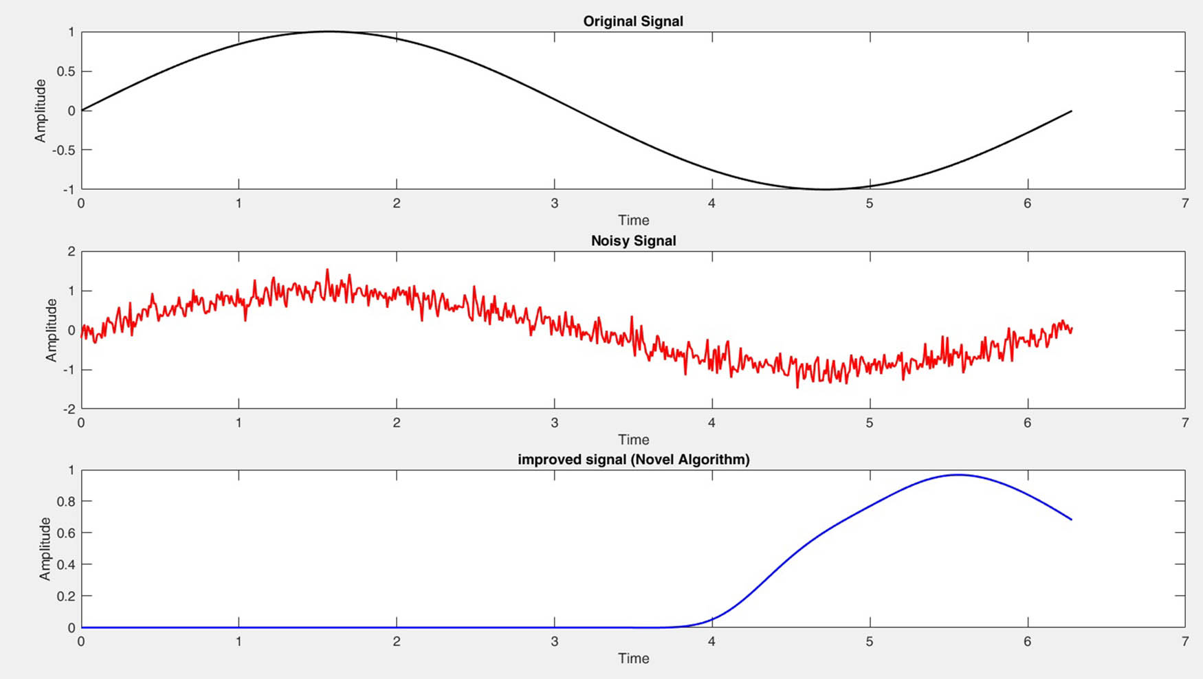
Original/noisy/enhanced signals as
Iterative methods adjust the signal in a balanced way, giving equal weight to both previous and current signals, which leads to a smoother and more progressive enhancement (Figure 3).
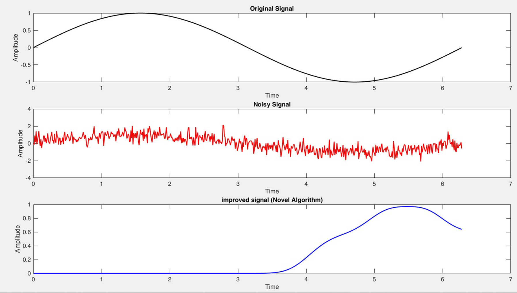
Original/noisy/enhanced signals as
If the learning rate is set too high, the algorithm might overadjust and fail to reach the optimal solution (Figure 4).
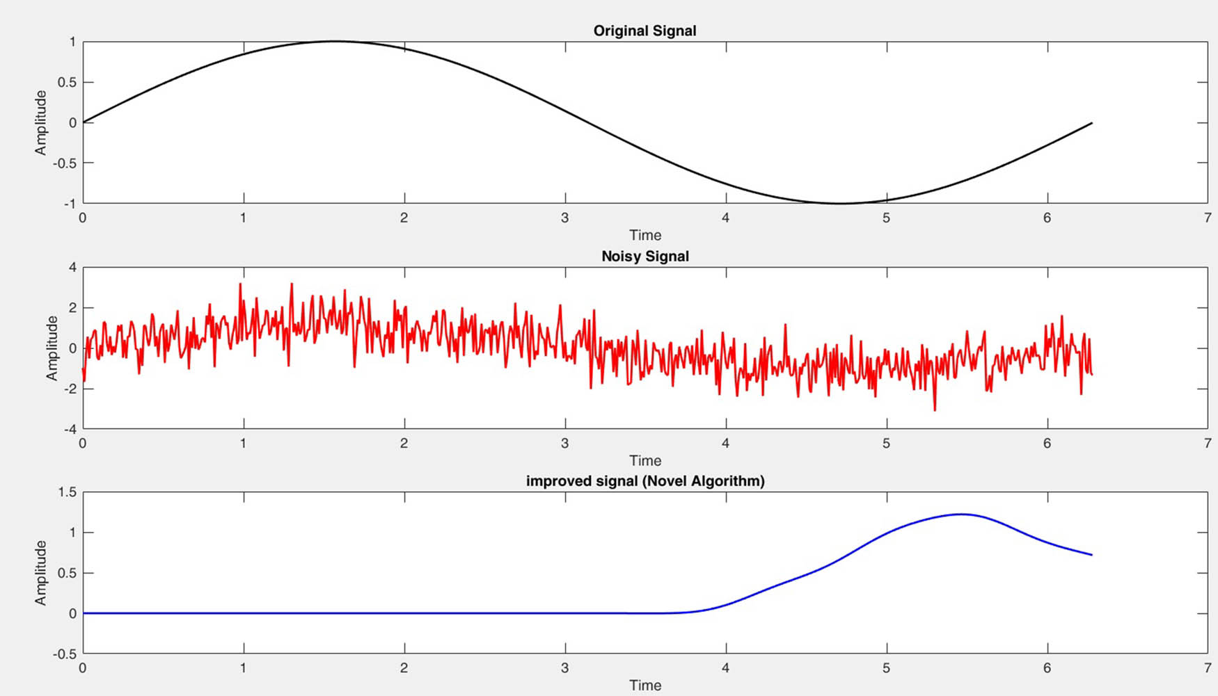
Original/noisy/enhanced signals as
The gradual refinement of the signal highlights the algorithm’s effective and stable noise reduction process. As the signal improves, it becomes increasingly clearer and eventually stabilizes, closely aligning with the original. This indicates that the algorithm is functioning properly, removing noise without excessively smoothing the signal [26,27].
Let’s explain the working logic of this code more clearly with a numerical example.
Example 5.1
Let’s take the learning rate as
These ten values are the first ten sample points of the enhanced signal
Comparison of original, noisy, and enhanced signal values for the first 10 time steps
| Step | Time (t) | Original signal | Noisy signal | Enhanced signal (after 50 iterations) |
|---|---|---|---|---|
| 1 | 0.00 |
|
|
0.0143 |
| 2 | 0.01 |
|
0.0724 | 0.0245 |
| 3 | 0.02 |
|
0.1911 | 0.0339 |
| 4 | 0.03 |
|
0.0950 | 0.0424 |
| 5 | 0.04 |
|
0.2034 | 0.0510 |
| 6 | 0.05 |
|
0.2780 | 0.0589 |
| 7 | 0.06 |
|
0.3397 | 0.0666 |
| 8 | 0.07 |
|
0.3072 | 0.0740 |
| 9 | 0.08 |
|
0.4892 | 0.0812 |
| 10 | 0.09 |
|
0.3921 | 0.0881 |
6 Convergence rate
In 1976, Rhoades [28] proposed a framework for evaluating the rate of convergence between two iterative algorithms, as outlined as follows:
Definition 6.1
[28] Let
In 2002, Berinde [29] applied the aforementioned concept to compare the rate of convergence between two iterative methods in the following manner:
Definition 6.2
[29] Let
(a) If
(b) If
Following the approach presented in [30], we provide an illustrative example to validate our findings and conduct a comparative analysis of the convergence rates between the proposed iteration scheme and the UO-iteration proposed by Okeke et al. [13].
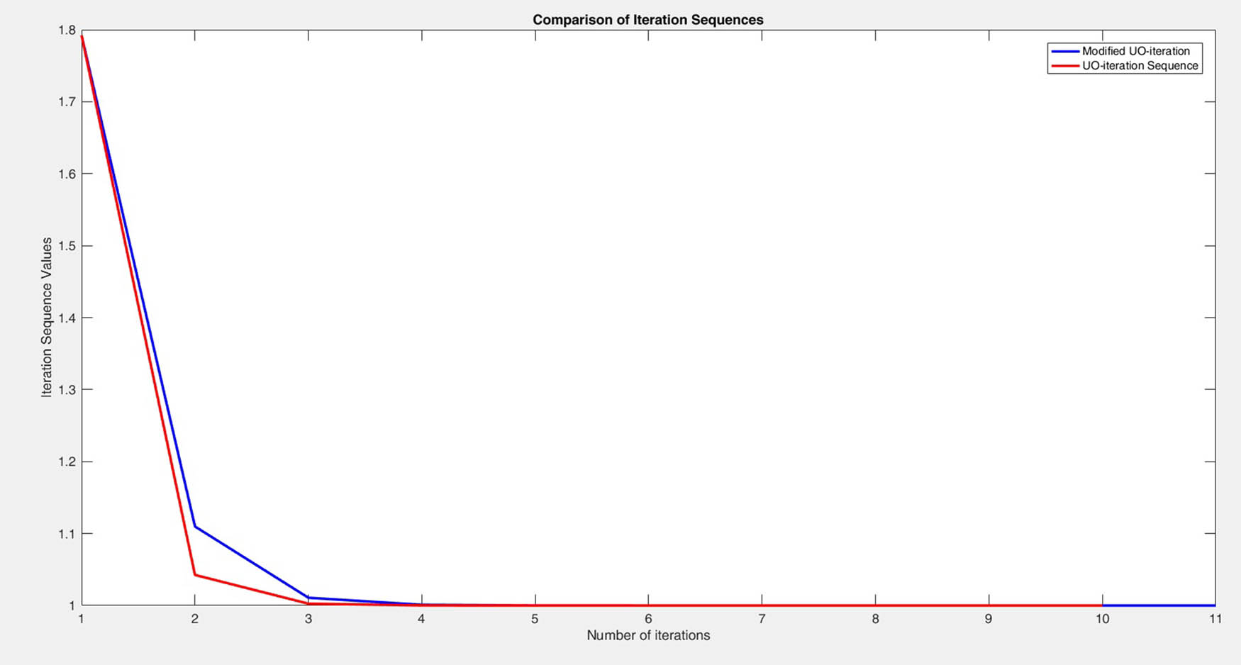
Example 6.3
Let
By using (1.1) and (1.2), we possess the numerical results to approximate the value of 1 as shown in Figure 5 with
Based on Tables 2 and 3, it can be inferred that
Numerical experiments for Example 6.3
|
|
(1.2) | (1.1) | Rate of convergence | ||
|---|---|---|---|---|---|
|
|
|
|
|
|
|
| 1 | 1.7923 | 1.7923 |
|
|
1 |
| 2 | 1.1098 | 1.0425 |
|
|
|
| 3 | 1.0108 | 1.0025 |
|
|
|
| 4 | 1.0010 | 1.0002 | 0.001 |
|
0.2 |
| 5 | 1.0001 | 1.0000 |
|
0 | 0 |
|
|
Rate (1.2) | (1.1) | ||
|---|---|---|---|---|
|
|
|
|
|
|
| 1 | 1.7923 | 0.6825 | 1.7923 | 0.7498 |
| 2 | 1.1098 | 0.099 | 1.0425 | 0.04 |
| 3 | 1.0108 | 0.0098 | 1.0025 | 0.0023 |
| 4 | 1.0010 | 0.0009 | 1.0002 | 0.0002 |
| 5 | 1.0001 | 0.0001 | 1.0000 | 0 |
The convergence of
7 Conclusion
Iterative algorithms are a key element in the image deblurring process. These algorithms progressively refine the image, providing an effective way to lessen blur and recover a result that closely mirrors the original. Beginning with the blurred image, they iteratively refine the solution, improving clarity with each step. On the other hand, signal enhancement and iterative algorithms are key components in contemporary engineering, where methods such as Bayesian enhancement, adaptive techniques, and filtering are employed to enhance signal clarity. These approaches are vital for minimizing noise and distortions, which in turn enhances the accuracy of results. Meanwhile, iterative methods are fundamental in the image deblurring process. These methods progressively refine the image over multiple iterations, gradually reducing blur and providing a clearer result that is closer to the original. Starting with a blurry image, each iteration works to improve and sharpen the output. Both signal enhancement and image recovery techniques will contribute to advancements in various areas, including satellite and remote sensing [31–34], autonomous systems [35,36], and medical imaging [37,38].
Acknowledgments
The author wishes to express profound appreciation to the reviewers for their detailed evaluations and recommendations, which greatly enriched the final version of this work.
-
Funding information: The author states no funding involved.
-
Author contribution: The author confirms the sole responsibility for the conception of the study, presented results, and manuscript preparation.
-
Conflict of interest: The author states no conflict of interest.
-
Data availability statement: No datasets were generated or analyzed during the current study.
References
[1] S. Banach, Sur les opérations dans les ensembles abstraits et leur application aux équations intégrales, Fund. Math. 3 (1922), 133–181, DOI: https://doi.org/10.4064/fm-3-1-133-181. 10.4064/fm-3-1-133-181Suche in Google Scholar
[2] J. Jachymski, The contraction principle for mappings on a metric space with a graph, Proc. Amer. Math. Soc. 136 (2008), 1359–1373, DOI: https://doi.org/10.1090/S0002-9939-07-09110-1. 10.1090/S0002-9939-07-09110-1Suche in Google Scholar
[3] R. Kelisky, T. Rivlin, Iterates of Bernstein polynomials, Pacific J. Math. 21 (1967), no. 3, 511–520. 10.2140/pjm.1967.21.511Suche in Google Scholar
[4] S. M. A. Aleomraninejad, S. Rezapour, and N. Shahzad, Some fixed point results on a metric space with a graph, Topology Appl. 159 (2012), 659–663, DOI: https://doi.org/10.1016/j.topol.2011.10.013. 10.1016/j.topol.2011.10.013Suche in Google Scholar
[5] M. R. Alfuraidan, M. A. Khamsi, Fixed points of monotone nonexpansive mappings on a hyperbolic metric space with a graph, Fixed Point Theory Appl. 2015 (2015), 44, DOI: https://doi.org/10.1186/s13663-015-0294-5. 10.1186/s13663-015-0294-5Suche in Google Scholar
[6] J. Tiammee, A. Kaewkhao, and S. Suantai, On Browder’s convergence theorem and Halpern iteration process for G-nonexpansive mappings in Hilbert spaces endowed with graphs, Fixed Point Theory Appl. 2015 (2015), 187, DOI: https://doi.org/10.1186/s13663-015-0436-9. 10.1186/s13663-015-0436-9Suche in Google Scholar
[7] O. Tripak, Common fixed points of G-nonexpansive mappings on Banach spaces with a graph, Fixed Point Theory Appl. 2016 (2016), 87, DOI: https://doi.org/10.1186/s13663-016-0578-4. 10.1186/s13663-016-0578-4Suche in Google Scholar
[8] R. Suparatulatorn, W. Cholamjiak, and S. Suantai, A modified S-iteration process for G-nonexpansive mappings in Banach spaces with graphs, Numer. Algorithms 77 (2018), no. 2, 479–490, DOI: https://doi.org/10.1007/s11075-017-0324-y. 10.1007/s11075-017-0324-ySuche in Google Scholar
[9] D. Yambangwai, T. Thianwan, Convergence point of G-nonexpansive mappings in Banach spaces endowed with graphs applicable in image deblurring and signal recovering problems, Ric. Mat. 73 (2024), 633–660, DOI: https://doi.org/10.1007/s11587-021-00631-y. 10.1007/s11587-021-00631-ySuche in Google Scholar
[10] C. Chairatsiripong, Y. Chonjaroen, D. Yambangwai, and T. Thianwan, Convergence analysis of M-iteration for G-nonexpansive mappings with directed graphs applicable in image deblurring and signal recovering problems, Demonstr. Math. 56 (2023), no. 1, 20220234, DOI: https://doi.org/10.1515/dema-2022-0234. 10.1515/dema-2022-0234Suche in Google Scholar
[11] D. Yambangwai, T. Thianwan, A parallel inertial SP-iteration monotone hybrid algorithm for a finite family of G-nonexpansive mappings and its application in linear system, differential, and signal recovery problems, Carpathian J. Math. 40 (2024), no. 2, 535–557, DOI: https://doi.org/10.37193/CJM.2024.02.19. 10.37193/CJM.2024.02.19Suche in Google Scholar
[12] S. Suantai, K. Kankam, W. Cholamjiak, and W. Yajai, Parallel hybrid algorithms for a finite family of G-nonexpansive mappings and its application in a novel signal recovery, Mathematics 10 (2022), 2140, DOI: https://doi.org/10.3390/math10122140. 10.3390/math10122140Suche in Google Scholar
[13] G. A. Okeke, A. V. Udo, N. H. Alharthi, and R. T. Alqahtani, A new robust iterative scheme applied in solving a fractional diffusion model for oxygen delivery via a capillary of tissues, Mathematics 12 (2024), 1339, DOI: https://doi.org/10.3390/math12091339. 10.3390/math12091339Suche in Google Scholar
[14] Z. Opial, Weak convergence of the sequence of successive approximations for nonexpansive mappings, Bull. Amer. Math. Soc. 73 (1967), 591–597, DOI: https://doi.org/10.1090/S0002-9904-1967-11761-0. 10.1090/S0002-9904-1967-11761-0Suche in Google Scholar
[15] N. Shahzad, A. Udomene, Approximating common fixed points of nonexpansive mappings in Banach spaces, Fixed Point Theory Appl. 2006 (2006), no. 1, 18909. 10.1155/FPTA/2006/18909Suche in Google Scholar
[16] K. K. Tan, H. K. Xu, Approximating fixed points of nonexpansive mapping by the Ishikawa iteration process, J. Math. Anal. Appl. 178 (1993), 301–308. 10.1006/jmaa.1993.1309Suche in Google Scholar
[17] J. Schu, Weak and strong convergence to fixed points of asymptotically nonexpansive mappings, Bull. Aust. Math. Soc. 43 (1991), 153–159. 10.1017/S0004972700028884Suche in Google Scholar
[18] S. Suantai, Weak and strong convergence criteria of Noor iterations for asymptotically nonexpansive mappings, J. Math. Anal. Appl. 331 (2005), 506–517. 10.1016/j.jmaa.2005.03.002Suche in Google Scholar
[19] K. Zhang, W. Ren, W. Luo, W. S. Lai, B. Stenger, M. H. Yang, et al., Deep image deblurring: a survey, Int. J. Comput. Vis. 130 (2022), 2103–2130, DOI: https://doi.org/10.1007/s11263-022-01633-5. 10.1007/s11263-022-01633-5Suche in Google Scholar
[20] S. B. Kang, Automatic removal of chromatic aberration from a single image, in Proc. IEEE Conf. Comput. Vis. Pattern Recognit. (CVPR), 2007. 10.1109/CVPR.2007.383214Suche in Google Scholar
[21] A. Abuolaim, M. S. Brown, Defocus Deblurring using dual-pixel data, in Proc. Eur. Conf. Comput. Vis. (ECCV), 2020. 10.1007/978-3-030-58607-2_7Suche in Google Scholar
[22] B. G. M. Vandeginste, D. L. Massart, L. M. C. Buydens, S. De Jong, P. J. Lewi, et al. Data Handling in Science and Technology, Ch. 40, Elsevier, Amsterdam, Netherlands, 1998, 507–574, DOI: https://doi.org/10.1016/S0922-3487(98)80050-6. 10.1016/S0922-3487(98)80050-6Suche in Google Scholar
[23] S. V. Vaseghi, Advanced Digital Signal Processing and Noise Reduction, John Wiley & Sons, Chichester, 2008. 10.1002/9780470740156Suche in Google Scholar
[24] C. Byrne, A unified treatment of some iterative algorithms in signal processing and image reconstruction, Inverse Problems 20 (2004), no. 1, 103, DOI: https://doi.org/10.1088/0266-5611/20/1/006. 10.1088/0266-5611/20/1/006Suche in Google Scholar
[25] J. A. Cadzow, Signal enhancement–a composite property mapping algorithm, IEEE Trans. Acoust. Speech Signal Process. 36 (1988), no. 1, 49–62, DOI: https://doi.org/10.1109/29.1488. 10.1109/29.1488Suche in Google Scholar
[26] J. G. Proakis, D. G. Manolakis, Digital Signal Processing: Principles, Algorithms, and Applications, Upper Saddle River, Prentice Hall, 2007. Suche in Google Scholar
[27] S. Haykin, Adaptive Filter Theory, Pearson, Upper Saddle River, NJ, USA, 2002. Suche in Google Scholar
[28] B. E. Rhoades, Comments on two fixed point iteration methods, J. Math. Anal. Appl. 56 (1976), no. 2, 741–750. 10.1016/0022-247X(76)90038-XSuche in Google Scholar
[29] V. Berinde, Iterative Approximation of Fixed Points, Lecture Notes in Mathematics, Springer-Verlag Berlin Heidelberg, Baia Mare, 2007, DOI: https://doi.org/10.1007/978-3-540-72234-2. 10.1007/978-3-540-72234-2Suche in Google Scholar
[30] R. Suparatulatorn, S. Suantai, and W. Cholamjiak, Hybrid methods for a finite family of G-nonexpansive mappings in Hilbert spaces endowed with graphs, AKCE Int. J. Graphs Comb. 14 (2017), no. 2, 101–111, DOI: https://doi.org/10.1016/j.akcej.2017.01.001. 10.1016/j.akcej.2017.01.001Suche in Google Scholar
[31] B. Rasti, Y. Chang, E. Dalsasso, L. Denis, and P. Ghamisi, Image restoration for remote sensing: overview and toolbox, IEEE Geosci. Remote Sens. Mag. 10 (2022), no. 2, 201–230, DOI: https://doi.org/10.1109/MGRS.2021.3121761. 10.1109/MGRS.2021.3121761Suche in Google Scholar
[32] N. K. Greeshma, M. Baburaj, and N. G. Sudhish, Reconstruction of cloud-contaminated satellite remote sensing images using kernel PCA-based image modelling, Arab. J. Geosci. 9 (2016), 239, DOI: https://doi.org/10.1007/s12517-015-2199-3. 10.1007/s12517-015-2199-3Suche in Google Scholar
[33] S. Zhong, X. Zhao, D. Liu, H. Su, Z. Xie, and B. Fan, High-resolution, lightweight remote sensing via harmonic diffractive optical imaging systems and deep denoiser prior image restoration, IEEE Trans. Geosci. Remote Sens. 62 (2024), 5621717, DOI: https://doi.org/10.1109/TGRS.2024.3394154. 10.1109/TGRS.2024.3394154Suche in Google Scholar
[34] C. H. Chen (Ed.), Signal and Image Processing for Remote Sensing, CRC Press, Boca Raton, 2012. 10.1201/b11656Suche in Google Scholar
[35] M. Jamshidi, Autonomous control systems: applications to remote sensing and image processing, in SPIE 4471, Algorithms and Systems for Optical Information Processing V, SPIE, Bellingham, WA, USA, 2001, DOI: https://doi.org/10.1117/12.449352. 10.1117/12.449352Suche in Google Scholar
[36] Z. Bairi, O. Ben-Ahmed, A. Amamra, A. Bradai, and K. B. Beghdad, PSCS-Net: Perception optimized image reconstruction network for autonomous driving systems, IEEE Trans. Intell. Transp. Syst. 24 (2023), no. 2, 1564–1579, DOI: https://doi.org/10.1109/TITS.2022.3223167. 10.1109/TITS.2022.3223167Suche in Google Scholar
[37] S. Tong, A. M. Alessio, and P. E. Kinahan, Image reconstruction for PET/CT scanners: past achievements and future challenges, Imaging Med. 2 (2010), no. 5, 529–545. 10.2217/iim.10.49Suche in Google Scholar PubMed PubMed Central
[38] Y. Liu, M. De Vos, I. Gligorijevic, V. Matic, Y. Li, and S. Van Huffel, Multi-structural signal recovery for biomedical compressive sensing, IEEE Trans. Biomed. Eng. 60 (2013), no. 10, 2794–2805, DOI: https://doi.org/10.1109/TBME.2013.2264772. 10.1109/TBME.2013.2264772Suche in Google Scholar PubMed
© 2025 the author(s), published by De Gruyter
This work is licensed under the Creative Commons Attribution 4.0 International License.
Artikel in diesem Heft
- On I-convergence of nets of functions in fuzzy metric spaces
- Special Issue on Contemporary Developments in Graphs Defined on Algebraic Structures
- Forbidden subgraphs of TI-power graphs of finite groups
- Finite group with some c#-normal and S-quasinormally embedded subgroups
- Classifying cubic symmetric graphs of order 88p and 88p 2
- Two-sided zero-divisor graphs of orientation-preserving and order-decreasing transformation semigroups
- Simplicial complexes defined on groups
- Further results on permanents of Laplacian matrices of trees
- Algebra
- Classes of modules closed under projective covers
- On the dimension of the algebraic sum of subspaces
- Green's graphs of a semigroup
- On an uncertainty principle for small index subgroups of finite fields
- On a generalization of I-regularity
- Algorithm and linear convergence of the H-spectral radius of weakly irreducible quasi-positive tensors
- The hyperbolic CS decomposition of tensors based on the C-product
- On weakly classical 1-absorbing prime submodules
- Equational characterizations for some subclasses of domains
- Algebraic Geometry
- Spin(8, ℂ)-Higgs bundles fixed points through spectral data
- Embedding of lattices and K3-covers of an Enriques surface
- Kodaira-Spencer maps for elliptic orbispheres as isomorphisms of Frobenius algebras
- Applications in Computer and Information Sciences
- Dynamics of particulate emissions in the presence of autonomous vehicles
- Exploring homotopy with hyperspherical tracking to find complex roots with application to electrical circuits
- Category Theory
- The higher mapping cone axiom
- Combinatorics and Graph Theory
- 𝕮-inverse of graphs and mixed graphs
- On the spectral radius and energy of the degree distance matrix of a connected graph
- Some new bounds on resolvent energy of a graph
- Coloring the vertices of a graph with mutual-visibility property
- Ring graph induced by a ring endomorphism
- A note on the edge general position number of cactus graphs
- Complex Analysis
- Some results on value distribution concerning Hayman's alternative
- Freely quasiconformal and locally weakly quasisymmetric mappings in metric spaces
- A new result for entire functions and their shifts with two shared values
- On a subclass of multivalent functions defined by generalized multiplier transformation
- Singular direction of meromorphic functions with finite logarithmic order
- Growth theorems and coefficient bounds for g-starlike mappings of complex order λ
- Refinements of inequalities on extremal problems of polynomials
- Control Theory and Optimization
- Averaging method in optimal control problems for integro-differential equations
- On superstability of derivations in Banach algebras
- The robust isolated calmness of spectral norm regularized convex matrix optimization problems
- Observability on the classes of non-nilpotent solvable three-dimensional Lie groups
- Differential Equations
- The ill-posedness of the (non-)periodic traveling wave solution for the deformed continuous Heisenberg spin equation
- A note on the global existence and boundedness of an N-dimensional parabolic-elliptic predator-prey system with indirect pursuit-evasion interaction
- Blow-up of solutions for Euler-Bernoulli equation with nonlinear time delay
- Periodic or homoclinic orbit bifurcated from a heteroclinic loop for high-dimensional systems
- Regularity of weak solutions to the 3D stationary tropical climate model
- Local minimizers for the NLS equation with localized nonlinearity on noncompact metric graphs
- Global existence and blow-up of solutions to pseudo-parabolic equation for Baouendi-Grushin operator
- Bubbles clustered inside for almost-critical problems
- Existence and multiplicity of positive solutions for multiparameter periodic systems
- Existence of positive periodic solutions for evolution equations with delay in ordered Banach spaces
- On a nonlinear boundary value problems with impulse action
- Normalized ground-states for the Sobolev critical Kirchhoff equation with at least mass critical growth
- Multiple positive solutions to a p-Kirchhoff equation with logarithmic terms and concave terms
- Infinitely many solutions for a class of Kirchhoff-type equations
- Real and non-real eigenvalues of regular indefinite Sturm–Liouville problems
- Existence of global solutions to a semilinear thermoelastic system in three dimensions
- Limiting profile of positive solutions to heterogeneous elliptic BVPs with nonlinear flux decaying to negative infinity on a portion of the boundary
- Morse index of circular solutions for repulsive central force problems on surfaces
- Differential Geometry
- On tangent bundles of Walker four-manifolds
- Pedal and negative pedal surfaces of framed curves in the Euclidean 3-space
- Discrete Mathematics
- Eventually monotonic solutions of the generalized Fibonacci equations
- Dynamical Systems Ergodic Theory
- Dynamical properties of two-diffusion SIR epidemic model with Markovian switching
- A note on weighted measure-theoretic pressure
- Pullback attractors for a class of second-order delay evolution equations with dispersive and dissipative terms on unbounded domain
- Pullback attractor of the 2D non-autonomous magneto-micropolar fluid equations
- Functional Analysis
- Spectrum boundary domination of semiregularities in Banach algebras
- Approximate multi-Cauchy mappings on certain groupoids
- Investigating the modified UO-iteration process in Banach spaces by a digraph
- Tilings, sub-tilings, and spectral sets on p-adic space
- Continuity and essential norm of operators defined by infinite tridiagonal matrices in weighted Orlicz and l∞ spaces
-
A family of commuting contraction semigroups on
- q-Stirling sequence spaces associated with q-Bell numbers
- Chlodowsky variant of Bernstein-type operators on the domain
- Hyponormality on a weighted Bergman space of an annulus with a general harmonic symbol
- Characterization of derivations on strongly double triangle subspace lattice algebras by local actions
- Fixed point approaches to the stability of Jensen’s functional equation
- Geometry
- The regularity of solutions to the Lp Gauss image problem
- Solving the quartic by conics
- Group Theory
- On a question of permutation groups acting on the power set
- A characterization of the translational hull of a weakly type B semigroup with E-properties
- Harmonic Analysis
- Eigenfunctions on an infinite Schrödinger network
- Maximal function and generalized fractional integral operators on the weighted Orlicz-Lorentz-Morrey spaces
- Subharmonic functions and associated measures in ℝn
- Mathematical Logic, Model Theory and Foundation
- A topology related to implication and upsets on a bounded BCK-algebra
- Boundedness of fractional sublinear operators on weighted grand Herz-Morrey spaces with variable exponents
- Number Theory
- Fibonacci vector and matrix p-norms
- Recurrence for probabilistic extension of Dowling polynomials
- Carmichael numbers composed of Piatetski-Shapiro primes in Beatty sequences
- The number of rational points of some classes of algebraic varieties over finite fields
- Classification and irreducibility of a class of integer polynomials
- Decompositions of the extended Selberg class functions
- Joint approximation of analytic functions by the shifts of Hurwitz zeta-functions in short intervals
- Fibonacci Cartan and Lucas Cartan numbers
- Recurrence relations satisfied by some arithmetic groups
- The hybrid power mean involving the Kloosterman sums and Dedekind sums
- Numerical Methods
- A modified predictor–corrector scheme with graded mesh for numerical solutions of nonlinear Ψ-caputo fractional-order systems
- A kind of univariate improved Shepard-Euler operators
- Probability and Statistics
- Statistical inference and data analysis of the record-based transmuted Burr X model
- Multiple G-Stratonovich integral in G-expectation space
- p-variation and Chung's LIL of sub-bifractional Brownian motion and applications
- Real Analysis
- Chebyshev polynomials of the first kind and the univariate Lommel function: Integral representations
- Multiple solutions for a class of fourth-order elliptic equations with critical growth
- Majorization-type inequalities for (m, M, ψ)-convex functions with applications
- The evaluation of a definite integral by the method of brackets illustrating its flexibility
- Some new Fejér type inequalities for (h, g; α - m)-convex functions
- Some new Hermite-Hadamard type inequalities for product of strongly h-convex functions on ellipsoids and balls
- Topology
- Unraveling chaos: A topological analysis of simplicial homology groups and their foldings
- A generalized fixed-point theorem for set-valued mappings in b-metric spaces
- On SI2-convergence in T0-spaces
- Generalized quandle polynomials and their applications to stuquandles, stuck links, and RNA folding