Robust estimation for partial functional linear regression models based on FPCA and weighted composite quantile regression

1 Introduction

In the literature of functional data analysis, functional linear regression models (FLRMs) provide an efficient method to analyze the relationship between a functional predictor and a scalar response. Therefore, much effort has been devoted to studying its estimation and other relevant inference problems, see [1,2, 3,4,5, 6,7,8, 9,10,11, 12,13]. However, in practice, we often see that a scalar response is related not only to functional covariates but also to scalar covariates. Thus, Shin considered partial functional linear regression models (PFLRMs) to balance the flexibility of FLRMs and interpretation of classical linear regression models [14]. Generally, PFLRM has the following form:

where Y is a real-valued response variable defined on a probability space ( Ω , ℬ , P ) , Z is a p -dimensional random vector and θ = ( θ 1 , … , θ p ) T is an unknown parameter vector, { X ( t ) ; t ∈ T } is a zero mean, second-order stochastic process defined on ( Ω , ℬ , P ) with sample paths in H = L 2 ( T ) , the Hilbert space containing square integrable functions on T with inner product ⟨ x , y ⟩ = ∫ T x ( t ) y ( t ) d t , ∀ x , y ∈ H and norm ‖ x ‖ = ⟨ x , x ⟩ 1 / 2 , β ( t ) is an unknown slope function belonging to H , ε is the random error independent of Z and X , E ( ε ∣ Z , X ) = 0 . T denotes the transport operation throughout this paper. Without loss of generality, we further assume T = [ 0 , 1 ] .

The PFLRMs have been studied by many authors. For example, Shin [14] proposed the estimation method based on functional principal component analysis (FPCA) and investigated the asymptotic properties of the estimators for model (1). Zhou et al. [15] considered the polynomial spline method to estimate model (1) and established the asymptotic normality for the parameter vector and the global convergence rate for the slope function. Furthermore, Kong et al. [16] studied variable selection in model (1) with multiple functional and ultrahigh-dimensional scalar predictors. Ling et al. [17] developed the k-nearest-neighbors estimation for PFLRMs. Kong et al. [18] proposed the partial functional linear cox regression model for censored outcomes. Cao et al. [19] developed a two-step estimation procedure via maximizing the quasi likelihood function in the framework of generalized PFLRMs. Yuan and Zhang [20] investigated the hypothesis test of the parametric components in PFLRMs based on B-spline. Zhu et al. [21] considered estimation and testing problems for PFLRMs when the covariates of the non-functional linear component are measured with additive error. Li et al. [22] proposed two test statistics for series correlation in PFLRMs and derived their asymptotic distributions under the null hypothesis.

Quantile regression (QR) is an effective approach for functional data analysis. This is due to the fact that QR models compared to the mean regression models [23] offer more robust merits especially the observations contain some outliers. For relevant literature, see [24,25,26]. Hence, QR method may result in an arbitrarily small relative efficiency compared with the mean regression. To conquer this drawback of QR method, Zou and Yuan proposed the composite quantile regression (CQR) method for linear models and showed that the relative efficiency of the CQR estimator is greater than 70% regardless of the error distribution compared with the least square (LS) estimator [27]. In many cases, CQR provides more efficient estimation compared with a single QR or the LS estimator for non-normal error distributions. This method has been deeply investigated in the literature and widely applied in many statistical models. For further references about the CQR method on nonparametric/semi-parametric models see [28,29,30, 31,32]. Even though CQR has been well developed, theory and methodology of PFLRMs are rare. Du et al. [33] used the penalized CQR method to study variable selection for parametric part in the PFLRMs, Yu et al. [34] considered composite quantile estimation for the PFLRMs with errors from short-range dependent and strictly stationary linear processes. However, the aforementioned CQR method for PFLRMs is a sum of different QRs with equal weights. Intuitively, using equal weights is not optimal in general, though CQR enjoys great advantages in terms of estimation efficiency. Therefore, Jiang et al. [35] addressed the issue of statistical inference for nonlinear models with large-dimensional covariates by using the weighted composite quantile regression (WCQR) method. Moreover, they pointed out that their method was more robust than some existing methods. Guo et al. [36] investigated group SCAD penalized WCQR estimation for varying coefficient models with diverging number of parameters. Jiang et al. [37] developed a data-driven WCQR for heteroscedastic partially linear varying coefficient models. Similar conclusions of WCQR method have been further confirmed in [6,38,39]. Until now, the WCQR method has not been used in functional regression analysis. Consequently, motivated by this fact, we devote to extending the WCQR method to PFLRMs in this paper. We show that the resulting estimators for both parametric components and slope function are more efficient in the case of asymmetrical error distribution, and as asymptotically efficient as the corresponding LS estimators when the error distribution is normal.

It is well known that many smoothing methods have been proposed for functional regressions, and two popular approaches for estimating the slope function β ( ⋅ ) include the FPCA approach based on spectral decompositions of both the covariance of X ( t ) and its estimator (see [3,7,40]) and the basis function expansion method with both β ( ⋅ ) and X ( t ) approximated by basis functions such as polynomial spline functions in [15]. In this paper, we propose a WCQR estimation method for PFLRMs through weighted composite quantile loss function with principal component basis function approximations. The main contributions of this paper are threefold:

1. This is the first attempt to provide robust estimate via WCQR and establish the asymptotic properties of the proposed estimators for model (1).

2. We develop a data-driven weighting strategy that maximizes the efficiency of the WCQR estimators. Practically, the proposed method is more efficient than the CQR method in [33] and rank regression method proposed under asymmetrical error distributed data set in [38].

3. Theoretically, the proposed WCQR method generalizes the results of the composite quantile estimators in [8]. Particularly, our method reduces to that of Du et al. when the weights are all equal.

The rest of this paper is organized as follows. In Section 2, we describe the implementation details of the proposed algorithm and establish the theoretical properties of the estimators. In Section 3, we discuss the selection of weights and tuning parameters. Simulation study and a real data analysis are conducted in Sections 4 and 5 to evaluate the performance of our proposed approach, and then followed by a short conclusion in Section 6. All technical proofs are collected in the Appendix.

2 Method and main results

In partial functional linear QR model, for a given quantile level τ ∈ ( 0 , 1 ) , ( Z i , X i ( ⋅ ) , Y i ) , i = 1 , … , n is an independent and identically distributed (i.i.d.) sample from model (1), that is

where Q τ ( Y ∣ Z , X ( t ) ) is the τ th conditional quantile of Y given ( Z , X ( t ) ) , Y is a real-valued random variable defined on a probability space ( Ω , ℬ , P ) , Z is a p -dimensional vector of random variables with finite second moments, θ τ is a p × 1 coefficient vector to be estimated, β τ ( t ) is an unknown square integrable function on [ 0 , 1 ], and ε τ is a random error whose τ th quantile conditional on ( Z , X ( t ) ) being zero. For the convenience of presentation, we will omit τ from θ τ , β τ ( t ) and ε τ in model (2) wherever clear from the context, but we should keep in mind that those quantities are τ -specific.

Denote the covariance function of the process X ( ⋅ ) and its empirical version, respectively, as

The covariance function K defines a linear operator which maps a function f to K f given by ( K f ) ( u ) = ∫ K ( u , v ) f ( v ) d v . We assume that the linear operator with kernel K is positive definite. By Mercer’s theorem, then

where λ 1 > λ 2 > ⋯ > 0 and λ ˆ 1 ≥ λ ˆ 2 ≥ ⋯ ≥ λ ˆ n + 1 = ⋯ = 0 are, respectively, the ordered eigenvalue sequences of the linear operators with kernels K and K ˆ , and { ϕ j } and { ϕ ˆ j } are the corresponding orthonormal eigenfunction sequences. Obviously, the vectors { ϕ j } and { ϕ ˆ j } each forms an orthonormal basis in H . According to the Karhunen-Loèvere presentation, then

where ξ i and γ i are defined by

where ξ i is referred to as the i th functional principal component score of X ( t ) . It follows that ξ i are uncorrelated random variables with mean 0 and variance E ( ξ i 2 ) = λ i . For more details see [41]. Substituting (3) into model (2), the model (2) can be written as

Therefore, the regression model in (4) can be well approximated by

where m ≤ n is the truncation level that trades off approximation error against variability and typically diverges with n . Replace ϕ j by ϕ ˆ j for j = 1 , … , m , model (5) can be rewritten as

where U = { ⟨ X , ϕ ˆ j ⟩ } j = 1 , … , m , γ = ( γ 1 , … , γ m ) T . Thus, the estimation problem of the parameters and the slope function are transformed into the estimation problem of the parameter vectors θ and γ .

Note that the CQR method used the same weight for different QR models. Intuitively, it will be more effective if different weights are used. According to Jiang et al. [35], the WCQR procedure estimates θ and γ via minimizing the following loss function:

where ρ τ k ( r ) = τ k r − r I ( r < 0 ) , k = 1 , … , q , q is the number of quantiles, τ k ∈ ( 0 , 1 ) . Typically, we use equally spaced quantile position: τ k = k / ( 1 + q ) , ω = ( ω 1 , … , ω q ) T is a vector of weight satisfying ω k ≥ 0 . c τ k is 100 τ k % quantile of ε , c = ( c τ 1 , … , c τ q ) T . Let the coefficients γ ^ = ( γ ^ 1 , … , γ ^ m ) T and θ ^ = ( θ ^ 1 , … , θ ^ p ) T be the solution of equation (6), then the resulting estimator of the slope function is given by

3 Assumptions and asymptotic results

To establish the asymptotic properties of the proposed estimators, first, we introduce some notations. Let θ 0 and β 0 ( t ) be the true values of θ and β ( t ) , respectively, the notation ‖ ⋅ ‖ is the L 2 norm for a function or the Euclidean norm for a vector. Let C denote a generic constant that might assume different values at different places, a n ∼ b n means that a n / b n is bounded away from 0 and infinity as n → ∞ . The following technical assumptions are imposed.

1. The random function X ( ⋅ ) satisfies E ∣ ∣ X ( ⋅ ) ∣ ∣ 4 < ∞ .

2. For each j , E [ U j 4 ] ≤ C λ j 2 . For the eigenvalues λ j and Fourier coefficients γ j , we require that λ j − λ j + 1 ≥ C − 1 j − a − 1 and ∣ γ j ∣ ≤ C j − b for j > 1 , a > 1 and b > a / 2 + 1 .

3. The tuning parameter m satisfies m ∼ n 1 / ( a + 2 b ) .

4. The random vector Z has bounded fourth moment, E ‖ Z ‖ 4 < ∞ .

5. Z = η + ⟨ g , X ⟩ , where η = ( η 1 , … , η p ) T is zero-mean random variable, g = ( g 1 , … , g p ) T with g j ∈ L 2 ( [ 0 , 1 ] ) , j = 1 , … , p .

6. E [ η ] = 0 and E [ η η T ] = Σ . Furthermore, we need that Σ is a positive definite matrix.

7. ε has the distribution function F ( ⋅ ) with density f ( ⋅ ) . The density function f ( ⋅ ) of ε is positive and continuous at the τ k th quantiles c τ k .

4 Computational issues

From Theorem 3.1, we find that the asymptotic variance of θ ^ depends on ω only through σ 2 ( ω ) . Thus, the optimal choice of weights for maximizing efficiency of the estimator θ ^ is ω opt = arg min ω σ 2 ( ω ) . Based on [36], the optimal choice of weights is to solve the following quadratic optimization problem:

where f = ( f ( c τ 1 ) , … , f ( c τ q ) ) T and Ω is a q × q matrix with the ( k , k ′ ) element Ω k , k ′ = min ( τ k , τ k ′ ) − τ k τ k ′ .

It can be seen from (8) that the optimal weight vector is rather complicated and involves the density of the errors c k = F − 1 ( τ k ) and f ( c k ) , k = 1 , … , q . In practice, the error density f ( ⋅ ) is generally unknown. Following [36], we propose an estimation procedure as follows.

Step 1. We give the initial estimators θ ˜ and β ˜ ( t ) by minimizing the LS objective function and estimate σ 2 ( ⋅ ) by

Step 2. Compute ε ˜ i = Y i − Z i T θ ˜ − ∫ 0 1 X i ( t ) β ˜ ( t ) d t σ ˜ and then we can use kernel density estimation to estimate f ( ⋅ ) as follows:

Similar to Silverman [42], the bandwidth h is taken as

K ( ⋅ ) is always chosen as the Gaussian kernel. Here std( ⋅ ) and IQR( ⋅ ) denote the sample standard deviation and sample interquartile, respectively.

Step 3. Estimate f { F − 1 ( τ k ) } by f ˜ { F ˜ − 1 ( τ k ) } , where F ˜ − 1 ( τ k ) is the sample τ k quantile of { ε ˜ i , i = 1 , … , n } .

The proposed estimators involve the tuning parameter m , which needs to be selected by minimizing some selection criteria such as cross validation (CV), generalized cross validation (GCV), AIC information criterion, BIC information criterion, etc. We use a BIC-type criterion to select m [36], that is

where p is the number of components in parameter vector. c ˆ τ k ( m ) , θ ˆ ( m ) , and γ ˆ ( m ) are obtained by minimizing equation (7) with the first m principal components.

5 Simulation study

In this section, we conduct a Monte Carlo simulation example to assess the finite sample performance of the proposed procedures. Moreover, we include four competitors in our comparisons: (1) the LS method [14], (2) the QR method (QR) with τ = 0.5 [24], (3) the rank regression (RR) method [43], (4) the composite quantile regression (CQR) method [33]. Following [30], the performance of CQR estimation does not depend sensitively on the choice of the number of quantiles q . For the sake of simplicity, we only consider q = 9 for CQR and WCQR method in our simulation. The data sets are generated from the following PFLRM:

where both Z i 1 and Z i 2 are standard normal with correlation coefficient 0.5, θ 1 = 0.8 and θ 2 = 2 . For the functional linear component, we take the same form as [40]. Specifically, the slope function β ( t ) = 2 sin ( π t / 2 ) + 3 2 sin ( 3 π t / 2 ) and X ( t ) = ∑ j = 1 100 ξ j v j ( t ) , where the ξ j are independently distributed as the normal with mean 0 and variances given by λ j = 10 ( ( j − 0.5 ) π ) − 2 , v j ( t ) = 2 sin ( ( j − 0.5 ) π t ) .

In order to show the robustness of our estimators, the following six different error distributions are considered: standard normal distribution N(0, 1), t (3) distribution that is used to produce heavy-tailed distribution, F distribution F(4, 6), exponential distribution Exp(1), Log normal distribution LN(0, 1), and Weibull distribution Wb(1, 1.5) are used to produce asymmetric error distributions.

To assess the performance of the estimated parameters, the following criteria are considered:

(1) the average value of the corresponding coefficients (MEAN);

(2) the sample standard deviation (SD);

(3) the median of absolute bias (ABISE). To assess the performance of the slope function, we consider the following square root of average square errors (RASE):

where { t k , k = 1 , … , n grid } are the grid points at which the slope function β ( ⋅ ) is evaluated. In our simulation experiments, we set n grid = 200 , 500 repetitions are carried out with sample size n = 100 , 200, 400. In addition, the range of the selected m is from 1 to 8. The simulation results are presented in Tables 1, 2, 3, 4, 5, 6. From Tables 1–6, we have the following findings: (1) As the sample size n increases, the ABISE, SD, and RASE values of all estimators decrease. As expected, increasing the sample size leads to a better performance of all estimators. (2) The standard errors become smaller and the estimators of MEANs for the parametric components are very close to the true values θ as n increases, due to the fact of root- n consistency of the parameter estimators. This result confirms the asymptotic property that the parameter estimators are asymptotically unbiased as given in Theorem 3.1. (3) When the error follows N(0, 1), LS is the best one among the five estimators and WCQR performs nearly as well as CQR and RR. Although the QR method with quantile being 0.5 have similar performances, the WCQR seems to be slightly better than QR in most scenarios. (4) When the error distribution is symmetrical, CQR, RR, and WCQR perform similarly and satisfactorily. For all asymmetric errors: F(4, 6), Exp(1), LN(0, 1), and Wb(1, 1.5), WCQR performs better than others.

6 Application to Tecator data

We illustrate the proposed approach by analyzing a real estate data set which is available at http://lib.stat.cmu.edu/datasets/tecator. The data have been widely used to predict fat content on samples of finely chopped meat [44,45,46]. For each food sample, the functional data consist of a 100-channel spectrum of absorbances recorded on a Tecator Infratec Food and Feed Analysis working in the wavelength range 850–1,050 nm by the near infrared transmission principle. More details on the data can be found in Ferraty and Vieu [47]. In this section, we construct the following PFLRM model:

We denote the scale of fat content as Y i , the protein content as Z i , the moisture content as U i , and the absorbances as X i ( t ) .

To evaluate the performance of the method, the sample is randomly divided into two subsamples: the training sample, I 1 = { ( X i , Y i , Z i , U i ) , ∣ I 1 ∣ = 165 } , where ∣ I 1 ∣ denotes the cardinality of I 1 and the remaining is test sample, I 2 = { ( X i , Y i , Z i , U i ) , ∣ I 2 ∣ = 50 } . To verify our robust estimation procedures, we reanalyzed this data set by including some outliers in the response variable. The case is considered through controlling the number of outliers and the values of outliers, we randomly generate κ outliers by increasing the value Y to Y + t ( κ = 20 , t = 5 ) . The training samples are used to estimate the parameters and the test samples are employed to verify the quality of predictions. For this, we compute the mean square error of prediction MSEP [44], which is defined by

where Y ˆ i is the predicted value based on the training sample and Var I 2 is the variance of response variables from test sample. We use different estimation methods to predict the fat content of a meat sample based on its protein and/or moisture contents and/or its NIT absorbance spectrum, and the corresponding average MSEPs based on 200 times randomly splits are shown in Table 7. Compared with other methods, the MSEP of our proposed method (WCQR) is relatively smaller. Meanwhile, based on random simulations, the average estimated weight is ω opt = ( 0.4287 , 0.07228 , 0.0119 , 0.0114 , 0.0624 , 0.0631 , 0.0244 , 0.0022 , 0 ) and the corresponding standard deviation is (0.1608, 0.0895, 0.0481, 0.0257, 0.0275, 0.0403, 0.0690, 0.1261, 0). From Figure 1, we can see that the estimated slope functions β ( t ) ˆ by our WCQR method and CQR method, respectively, and it demonstrates that the two estimation approaches perform similarly.

Figure 1

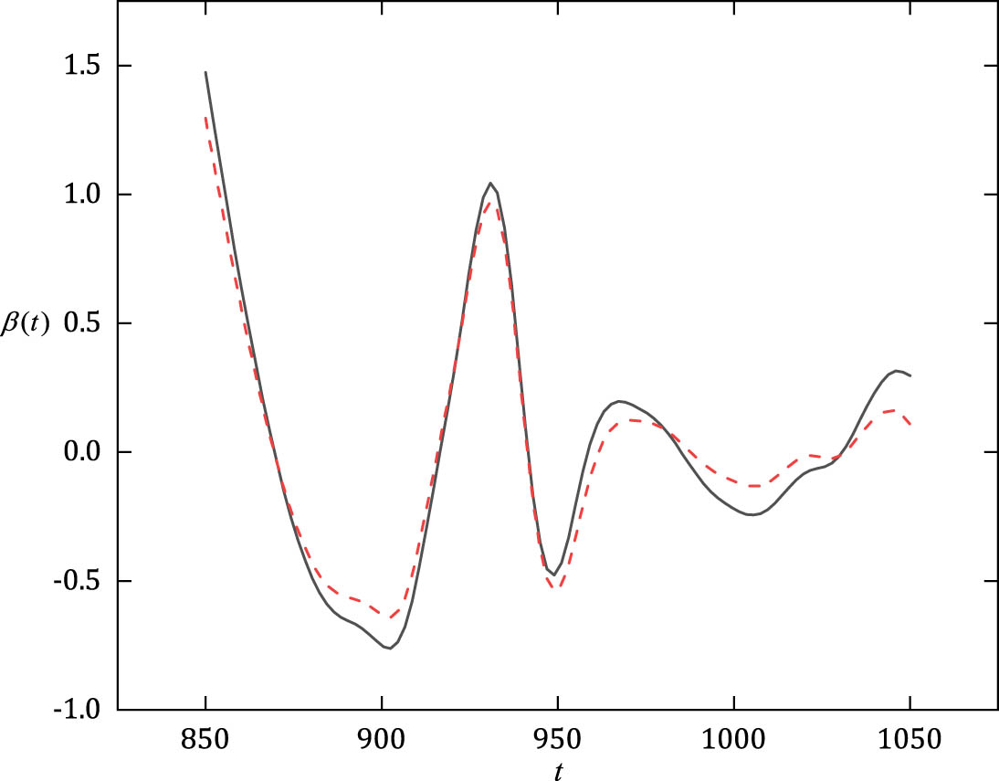
Curves of slope function β ( t ) ˆ with CQR (solid line) and WCQR (dotted line).

7 Conclusion

In this paper, a novel and robust procedure based on WCQR and principal component basis function approximations is developed for PFLRMs. Theoretical properties of the estimators of both slope function and linear parameters are derived under some mild assumptions. We show that the estimators do not require any specification for error distribution, and thus more robust than those based on the LS, QR and CQR in the case of asymmetric errors. Furthermore, we present an efficient algorithm for the selection of optimal weights and discuss the selection of tuning parameters. Numerical studies and the real data analysis illustrate that our proposed method performs very well for moderate sample size.

In addition, we could extend the proposed procedure to the functional regression models with diverse dimension of covariates. These deserve to be studied further.

References

[1] H. Cardot , F. Ferraty , and P. Sarda , Functional linear model, Statist. Probab. Lett. 45 (1999), no. 1, 11–22, https://doi.org/10.1016/S0167-7152(99)00036-X . 10.1016/S0167-7152(99)00036-XSearch in Google Scholar
[2] H. Cardot , F. Ferraty , and P. Sarda , Spline estimators for the functional linear model, Statist. Sinica 13 (2003), no. 3, 571–591, http://www.jstor.org/stable/24307112. Search in Google Scholar
[3] F. Yao , H. G. Müller , and J. L. Wang , Functional linear regression analysis for longitudinal data, Ann. Statist. 33 (2005), no. 6, 2873–2903, https://doi.org/10.1214/009053605000000660. Search in Google Scholar
[4] J. Ramsay and B. Silverman , Functional Data Analysis, 2nd edn., Springer, New York, 2005. 10.1007/b98888Search in Google Scholar
[5] T. Cai and P. Hall , Prediction in functional linear regression, Ann. Statist. 34 (2006), no. 5, 2159–2179, https://doi.org/10.1214/009053606000000830 . 10.1214/009053606000000830Search in Google Scholar
[6] H. Liu and H. Yang , Estimation and variable selection in single-index composite quantile regression, Comm. Statist. Simulation Comput. 46 (2016), no. 9, 7022–7039. 10.1080/03610918.2016.1222424Search in Google Scholar
[7] P. Hall and J. Horowitz , Methodology and convergence rates for functional linear regression, Ann. Statist. 35 (2007), no. 1, 70–91, https://doi.org/10.1214/009053606000000957. Search in Google Scholar
[8] C. Crambes , A. Kneip , and P. Sarda , Smoothing splines estimators for functional linear regression, Ann. Statist. 37 (2009), no. 1, 35–72, https://doi.org/10.1214/07-AOS563. Search in Google Scholar
[9] P. Hall and Y. Yang , Ordering and selecting components in multivariate or functional data linear prediction, J. R. Stat. Soc. Ser. B. Stat. Methodol. 72 (2010), no. 1, 93–110. 10.1111/j.1467-9868.2009.00727.xSearch in Google Scholar
[10] T. Cai and M. Yuan , Minimax and adaptive prediction for functional linear regression, J. Amer. Statist. Assoc. 107 (2012), no. 499, 1201–1216, https://www.jstor.org/stable/23427425. 10.1080/01621459.2012.716337Search in Google Scholar
[11] A. Delaigle and P. Hall , Methodology and theory for partial least squares applied to functional data, Ann. Statist. 40 (2012), no. 1, 322–352, https://doi.org/10.1214/11-AOS958. Search in Google Scholar
[12] E. R. Lee and B. U. Park , Sparse estimation in functional linear regression, J. Multivariate Anal. 105 (2012), no. 1, 1–17, https://doi.org/10.1016/j.jmva.2011.08.005. Search in Google Scholar
[13] L. Huang , H. Wang , and A. Zheng , The M-estimator for functional linear regression model, Statist. Probab. Lett. 88 (2014), no. C, 165–173, https://doi.org/10.1016/j.spl.2014.01.016. Search in Google Scholar
[14] H. J. Shin , Partial functional linear regression, J. Statist. Plann. Inference 139 (2009), no. 10, 3405–3418, https://doi.org/10.1016/j.jspi.2009.03.001 . 10.1016/j.jspi.2009.03.001Search in Google Scholar
[15] J. Zhou , Z. Chen , and Q. Peng , Polynomial spline estimation for partial functional linear regression models, Comput. Statist. 31 (2016), no. 3, 1107–1129, https://doi.org/10.1007/s00180-015-0636-0. Search in Google Scholar
[16] D. Kong , K. Xue , F. Yao , and H. Zhang , Partially functional linear regression in high dimensions, Biometrika 103 (2016), no. 1, 147–159, https://doi.org/10.1093/biomet/asv062. Search in Google Scholar
[17] N. Ling , G. Aneiros , and P. Vieu , kNN estimation in functional partial linear modeling, Statist. Papers 61 (2020), no. 1, 423–444, https://doi.org/10.1007/s00362-017-0946-0. Search in Google Scholar
[18] D. Kong , J. Ibrahim , E. Lee , and H. Zhu , FLCRM: functional linear cox regression model, Biometrics 74 (2018), no. 1, 109–117. 10.1111/biom.12748Search in Google Scholar PubMed PubMed Central
[19] R. Cao , J. Du , J. Zhou , and T. Xie , FPCA-based estimation for generalized functional partially linear models, Statist. Papers 61 (2020), no. 6, 2715–2735, https://doi.org/10.1007/s00362-018-01066-8. Search in Google Scholar
[20] M. Yuan and Y. Zhang , Test for the parametric part in partial functional linear regression based on B-spline, Comm. Statist. Simulation Comput. 50 (2021), no. 1, 1–15, https://doi.org/10.1080/03610918.2019.1667391. Search in Google Scholar
[21] H. Zhu , R. Zhang , Z. Yu , H. Lian , and Y. Liu , Estimation and testing for partially functional linear errors-in-variables models, J. Multivariate Anal. 170 (2019), 296–314, https://doi.org/10.1016/j.jmva.2018.11.005. Search in Google Scholar
[22] Q. Li , X. Tan , and L. Wang , Testing for error correlation in partially functional linear regression models, Comm. Statist. Theory Methods 50 (2021), no. 3, 747–761, https://doi.org/10.1080/03610926.2019.1642492 . 10.1080/03610926.2019.1642492Search in Google Scholar
[23] R. Koenker and G. Basset , Regression quantiles, Econometrica 46 (1978), no. 1, 33–50, https://doi.org/10.2307/1913643 . 10.2307/1913643Search in Google Scholar
[24] Y. Lu , J. Du , Z. Sun , Functional partially linear quantile regression model, Metrika 77 (2014), no. 2, 317–332, https://doi.org/10.1007/s00184-013-0439-7. Search in Google Scholar
[25] H. Ma , T. Li , H. Zhu , and Z. Zhu , Quantile regression for functional partially linear model in ultra-high dimensions, Comput. Statist. Data Anal. 129 (2019), no. 1, 135–147, https://doi.org/10.1016/j.csda.2018.06.005. Search in Google Scholar
[26] R. Koenker , Quantile Regression, Cambridge University Press, Cambridge, 2005. 10.1017/CBO9780511754098Search in Google Scholar
[27] H. Zou and M. Yuan , Composite quantile regression and the Oracle model selection theory, Ann. Statist. 36 (2008), no. 3, 1108–1126, https://www.jstor.org/stable/25464661. 10.1214/07-AOS507Search in Google Scholar
[28] B. Kai , R. Li , and H. Zou , Local composite quantile regression smoothing: an efficient and safe alternative to local polynomial regression, J. R. Stat. Soc. Ser. B Stat. Methodol. 72 (2010), no. 1, 49–69, https://doi.org/10.1111/j.1467-9868.2009.00725.x. Search in Google Scholar PubMed PubMed Central
[29] B. Kai , R. Li , and H. Zou , New efficient estimation and variable selection methods for semiparametric varying-coefficient partially linear models, Ann. Statist. 39 (2011), no. 1, 305–332, https://doi.org/10.1214/10-AOS842. Search in Google Scholar PubMed PubMed Central
[30] J. Guo , M. Tang , M. Tian , and K. Zhu , Variable selection in high-dimensional partially linear additive models for composite quantile regression, Comput. Statist. Data Anal. 65 (2013), 56–67, https://doi.org/10.1016/j.csda.2013.03.017. Search in Google Scholar
[31] R. Jiang , Z. Zhou , W. Qian , and Y. Chen , Two step composite quantile regression for single-index models, Comput. Statist. Data Anal. 64 (2013), 180–191, https://doi.org/10.1016/j.csda.2013.03.014. Search in Google Scholar
[32] R. Jiang , W. Qian , and Z. Zhou , Test for single-index composite quantile regression, Hacet. J. Math. Stat. 43 (2014), no. 5, 861–871. Search in Google Scholar
[33] J. Du , D. Xu , and R. Cao , Estimation and variable selection for partially functional linear models, J. Korean Statist. Soc. 47 (2018), no. 4, 436–449, https://doi.org/10.1016/j.jkss.2018.05.002. Search in Google Scholar
[34] P. Yu , T. Li , Z. Zhu , and Z. Zhang , Composite quantile estimation in partial functional linear regression model with dependent errors, Metrika 82 (2019), no. 6, 633–656, https://doi.org/10.1007/s00184-018-0699-3. Search in Google Scholar
[35] X. Jiang , J. Jiang , and X. Song , Oracle model selection for nonlinear models based on weighted composite quantile regression, Statist. Sinica 22 (2012), no. 4, 1479–1506, https://doi.org/10.5705/ss.2010.203. Search in Google Scholar
[36] C. Guo , H. Yang , and J. Lv , Robust variable selection in high-dimensional varying coefficient models based on weighted composite quantile regression, Statist. Papers 58 (2017), no. 4, 1009–1033, https://doi.org/10.1007/s00362-015-0736-5. Search in Google Scholar
[37] R. Jiang , W. Qian , and Z. Zhou , Weighted composite quantile regression for partially linear varying coefficient models, Comm. Statist. Theory Methods 47 (2018), no. 16, 3987–4005, https://doi.org/10.1080/03610926.2017.1366522. Search in Google Scholar
[38] J. Sun , Y. Gai , and L. Lin , Weighted local linear composite quantile estimation for the case of general error distributions, J. Statist. Plann. Inference 143 (2013), no. 6, 1049–1063, https://doi.org/10.1016/j.jspi.2013.01.002. Search in Google Scholar
[39] R. Jiang , W. Qian , and Z. Zhou , Weighted composite quantile regression for single-index models, J. Multivariate Anal. 148 (2016), 34–48, https://doi.org/10.1016/j.jmva.2016.02.015. Search in Google Scholar
[40] P. Yu , Z. Zhang , and J. Du , A test of linearity in partial functional linear regression, Metrika 79 (2016), no. 8, 953–969, https://doi.org/10.1007/s00184-016-0584-x. Search in Google Scholar
[41] L. Horváth and P. Kokoszka , Inference for Functional Data with Applications, Springer, New York, 2012. 10.1007/978-1-4614-3655-3Search in Google Scholar
[42] B. Silverman , Density Estimation, Chapman and Hall, London, 1986. Search in Google Scholar
[43] J. Sun and L. Lin , Local rank estimation and related test for varying-coefficient partially linear models, J. Nonparametr. Stat. 26 (2014), no. 1, 187–206, https://doi.org/10.1080/10485252.2013.841910. Search in Google Scholar
[44] G. Aneiros-Pérez and P. Vieu , Semi-functional partial linear regression, Statist. Probab. Lett. 76 (2006), no. 11, 1102–1110, https://doi.org/10.1016/j.spl.2005.12.007. Search in Google Scholar
[45] G. Aneiros-Pérez and P. Vieu , Partial linear modelling with multi-functional covariates, Comput. Statist. 30 (2015), no. 3, 647–671, https://doi.org/10.1007/s00180-015-0568-8. Search in Google Scholar
[46] P. Yu , J. Du , and Z. Zhan , Single-index partially functional linear regression model, Statist. Papers 61 (2020), no. 3, 1107–1123, https://doi.org/10.1007/s00362-018-0980-6. Search in Google Scholar
[47] F. Ferraty and P. Vieu , Nonparametric Functional Data Analysis: Theory and Practice, Springer, New York, 2006. Search in Google Scholar
[48] C. Crambes , A. Kneip , and P. Sarda , Smoothing splines estimators for functional linear regression, Ann. Statist. 37 (2009), no. 1, 35–72, https://doi.org/10.1214/07-AOS563. Search in Google Scholar
[49] K. Knight , Limiting distributions for L1 regression estimators under general conditions, Ann. Statist. 26 (1998), no. 2, 755–770, https://www.jstor.org/stable/120050.10.1214/aos/1028144858Search in Google Scholar
© 2021 Peng Cao and Jun Sun, published by De Gruyter
This work is licensed under the Creative Commons Attribution 4.0 International License.
Articles in the same Issue
- Regular Articles
- Sharp conditions for the convergence of greedy expansions with prescribed coefficients
- Range-kernel weak orthogonality of some elementary operators
- Stability analysis for Selkov-Schnakenberg reaction-diffusion system
- On non-normal cyclic subgroups of prime order or order 4 of finite groups
- Some results on semigroups of transformations with restricted range
- Quasi-ideal Ehresmann transversals: The spined product structure
- On the regulator problem for linear systems over rings and algebras
- Solvability of the abstract evolution equations in Ls-spaces with critical temporal weights
- Resolving resolution dimensions in triangulated categories
- Entire functions that share two pairs of small functions
- On stochastic inverse problem of construction of stable program motion
- Pentagonal quasigroups, their translatability and parastrophes
- Counting certain quadratic partitions of zero modulo a prime number
- Global attractors for a class of semilinear degenerate parabolic equations
- A new implicit symmetric method of sixth algebraic order with vanished phase-lag and its first derivative for solving Schrödinger's equation
- On sub-class sizes of mutually permutable products
- Asymptotic solution of the Cauchy problem for the singularly perturbed partial integro-differential equation with rapidly oscillating coefficients and with rapidly oscillating heterogeneity
- Existence and asymptotical behavior of solutions for a quasilinear Choquard equation with singularity
- On kernels by rainbow paths in arc-coloured digraphs
- Fully degenerate Bell polynomials associated with degenerate Poisson random variables
- Multiple solutions and ground state solutions for a class of generalized Kadomtsev-Petviashvili equation
- A note on maximal operators related to Laplace-Bessel differential operators on variable exponent Lebesgue spaces
- Weak and strong estimates for linear and multilinear fractional Hausdorff operators on the Heisenberg group
- Partial sums and inclusion relations for analytic functions involving (p, q)-differential operator
- Hodge-Deligne polynomials of character varieties of free abelian groups
- Diophantine approximation with one prime, two squares of primes and one kth power of a prime
- The equivalent parameter conditions for constructing multiple integral half-discrete Hilbert-type inequalities with a class of nonhomogeneous kernels and their applications
- Boundedness of vector-valued sublinear operators on weighted Herz-Morrey spaces with variable exponents
- On some new quantum midpoint-type inequalities for twice quantum differentiable convex functions
- Quantum Ostrowski-type inequalities for twice quantum differentiable functions in quantum calculus
- Asymptotic measure-expansiveness for generic diffeomorphisms
- Infinitesimals via Cauchy sequences: Refining the classical equivalence
- The (1, 2)-step competition graph of a hypertournament
- Properties of multiplication operators on the space of functions of bounded φ-variation
- Disproving a conjecture of Thornton on Bohemian matrices
- Some estimates for the commutators of multilinear maximal function on Morrey-type space
- Inviscid, zero Froude number limit of the viscous shallow water system
- Inequalities between height and deviation of polynomials
- New criteria-based ℋ-tensors for identifying the positive definiteness of multivariate homogeneous forms
- Determinantal inequalities of Hua-Marcus-Zhang type for quaternion matrices
- On a new generalization of some Hilbert-type inequalities
- On split quaternion equivalents for Quaternaccis, shortly Split Quaternaccis
- On split regular BiHom-Poisson color algebras
- Asymptotic stability of the time-changed stochastic delay differential equations with Markovian switching
- The mixed metric dimension of flower snarks and wheels
- Oscillatory bifurcation problems for ODEs with logarithmic nonlinearity
- The B-topology on S∗-doubly quasicontinuous posets
- Hyers-Ulam stability of isometries on bounded domains
- Inhomogeneous conformable abstract Cauchy problem
- Path homology theory of edge-colored graphs
- Refinements of quantum Hermite-Hadamard-type inequalities
- Symmetric graphs of valency seven and their basic normal quotient graphs
- Mean oscillation and boundedness of multilinear operator related to multiplier operator
- Numerical methods for time-fractional convection-diffusion problems with high-order accuracy
- Several explicit formulas for (degenerate) Narumi and Cauchy polynomials and numbers
- Finite groups whose intersection power graphs are toroidal and projective-planar
- On primitive solutions of the Diophantine equation x2 + y2 = M
- A note on polyexponential and unipoly Bernoulli polynomials of the second kind
- On the type 2 poly-Bernoulli polynomials associated with umbral calculus
- Some estimates for commutators of Littlewood-Paley g-functions
- Construction of a family of non-stationary combined ternary subdivision schemes reproducing exponential polynomials
- On the evolutionary bifurcation curves for the one-dimensional prescribed mean curvature equation with logistic type
- On intersections of two non-incident subgroups of finite p-groups
- Global existence and boundedness in a two-species chemotaxis system with nonlinear diffusion
- Finite groups with 4p2q elements of maximal order
- Positive solutions of a discrete nonlinear third-order three-point eigenvalue problem with sign-changing Green's function
- Power moments of automorphic L-functions related to Maass forms for SL3(ℤ)
- Entire solutions for several general quadratic trinomial differential difference equations
- Strong consistency of regression function estimator with martingale difference errors
- Fractional Hermite-Hadamard-type inequalities for interval-valued co-ordinated convex functions
- Montgomery identity and Ostrowski-type inequalities via quantum calculus
- Universal inequalities of the poly-drifting Laplacian on smooth metric measure spaces
- On reducible non-Weierstrass semigroups
- so-metrizable spaces and images of metric spaces
- Some new parameterized inequalities for co-ordinated convex functions involving generalized fractional integrals
- The concept of cone b-Banach space and fixed point theorems
- Complete consistency for the estimator of nonparametric regression model based on m-END errors
- A posteriori error estimates based on superconvergence of FEM for fractional evolution equations
- Solution of integral equations via coupled fixed point theorems in 𝔉-complete metric spaces
- Symmetric pairs and pseudosymmetry of Θ-Yetter-Drinfeld categories for Hom-Hopf algebras
- A new characterization of the automorphism groups of Mathieu groups
- The role of w-tilting modules in relative Gorenstein (co)homology
- Primitive and decomposable elements in homology of ΩΣℂP∞
- The G-sequence shadowing property and G-equicontinuity of the inverse limit spaces under group action
- Classification of f-biharmonic submanifolds in Lorentz space forms
- Some new results on the weaving of K-g-frames in Hilbert spaces
- Matrix representation of a cross product and related curl-based differential operators in all space dimensions
- Global optimization and applications to a variational inequality problem
- Functional equations related to higher derivations in semiprime rings
- A partial order on transformation semigroups with restricted range that preserve double direction equivalence
- On multi-step methods for singular fractional q-integro-differential equations
- Compact perturbations of operators with property (t)
- Entire solutions for several complex partial differential-difference equations of Fermat type in ℂ2
- Random attractors for stochastic plate equations with memory in unbounded domains
- On the convergence of two-step modulus-based matrix splitting iteration method
- On the separation method in stochastic reconstruction problem