On the evolutionary bifurcation curves for the one-dimensional prescribed mean curvature equation with logistic type
-
Jiajia Zhang
 ,
Lijuan Duan
,
Lijuan Duan

Abstract
We study the bifurcation diagrams and exact multiplicity of positive solutions for the one-dimensional prescribed mean curvature equation
where
1 Introduction
In this paper, we study the bifurcation curve and multiplicity of positive solutions for the one-dimensional prescribed mean curvature problem
where
Relative to the quasilinear equation (1.1), there is another semilinear equation
which has also received much attention in recent years [20,21,22, 23,24,25]. For equation (1.2), one parameter is actually enough because a scale of variable
General
In this paper, we consider the nonlinearity function
where the constant
For (1.3), we have
The nonlinearity
If
If
We always allow that solutions
We focus on the quasilinear problem (1.1)(1.3) as it is different from the following semilinear problems on the bifurcation curves:
While
at
Reversed S-shaped: We say that, on the
at
at
Reversed S-like shaped: On the
The paper is organized as follows. Section 2 contains statements of main results. Section 3 contains several lemmas needed to prove the main results. Finally, Section 4 contains the proofs of the main results.
2 Main results
The main results in this paper are Theorems 1–3 of (1.1)(1.3) with
First, let
with the initial-boundary conditions
Then we have the energy conservation relation
and
Here,
In terms of
Theorem 1
(Figure 1) Consider positive solutions
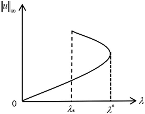
Theorem 2
(Figure 2) Consider positive solutions
when
when

Theorem 3
(Figure 3) Consider positive solutions
If
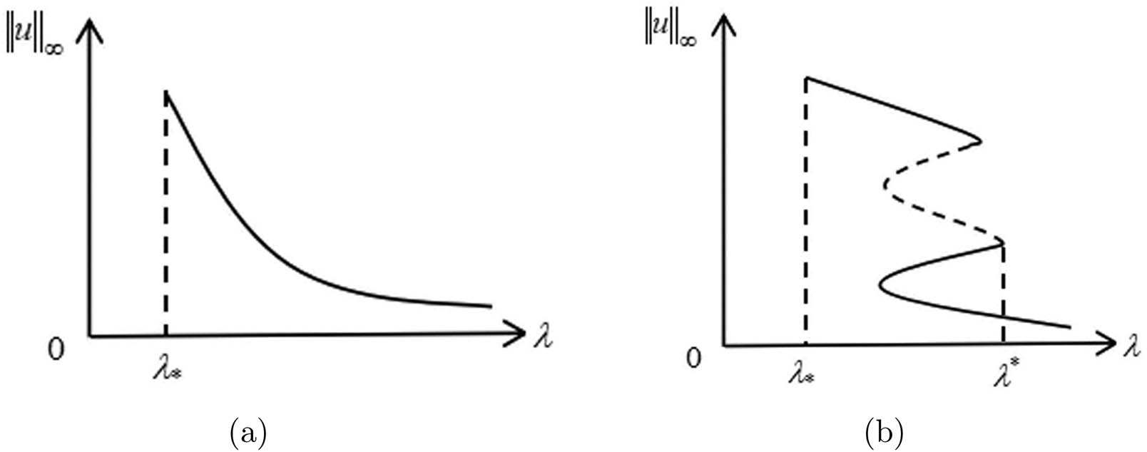
Bifurcation curves with
3 Lemmas
To prove Theorems 1–3, we make a detailed analysis of the time map for one-dimensional prescribed mean curvature problem (1.1)(1.3). The time-map method was applied by many authors of [2,9]. In this section, we define the time map formula for (1.1) by
Note that it can be proved that
First, we determine the limits of
Lemma 3.1
For (1.1)(1.3), for any fixed
and
Next, we determine
Proof
Since
and
using [31, Lemma 2.5], we get
Denote
Lemma 3.3
For (1.1)(1.3),
Proof
First, according to [2, Proposition 2.8],
Let
Then
and
Therefore,
Second, since
Define
Lemma 3.4
for fixed
Next, we will prove the general diagram of
Lemma 3.5
For (1.1)(1.3),
Proof
If
where
And
where
Since
Let
In terms of
then
Note that
then
Therefore,
As
Next, we need to determine the sign of
and
From (3.6), we have
and
Then the discriminant
By the above analysis, when
If
Lemma 3.6
For (1.1)(1.3) with
Proof
When
and
Note that
and
The proof of Lemma 3.6 is completed.□
For (3.1), we have
where
Note that
and
The graph of

The graph of
Let
Lemma 3.7
For (1.1)(1.3), when
Proof
Since
This completes the proof of Lemma 3.7.□
Then we study the profile of
From [4, Lemma 3.10], we have
From Lemmas 3.1 and 3.2,
4 Proof of main results
Proof of Theorem 1
If
For any
For any fixed
Moreover, there exists a unique
Then
The proof of Theorem 1 is completed.□
Proof of Theorem 2
If
For any
For any fixed
Let
Let
Next, we need to compare the endpoint value
so when
then
The proof of statement (1) is complete.
As
so when
then
The proof of Theorem 2 is completed.□
Proof of Theorem 3
If
For any
For any fixed
Note that
there exists
There exists a unique constant
Remark 1
It may be suggested from Theorems 1–3 that (a)
If
If
If
Acknowledgements
This research was supported by Beijing Municipal Natural Science Foundation (No. 4202025), partially sponsored by the National Natural Science Foundation of China (No. 61672070), Beijing Municipal Education Commission (No. KZ201910005008, KM201911232003), and the Research Fund from Beijing Innovation Center for Future Chips (No. KYJJ2018004).
-
Conflict of interest: Authors state no conflict of interest.
References
[1] P. Habets and P. Omari , Multiple positive solutions of a one-dimensional prescribed mean curvature problem, Commun. Contemp. Math. 9 (2007), no. 5, 701–730, https://doi.org/10.1142/S0219199707002617. Search in Google Scholar
[2] H. Pan and R. Xing , Time maps and exact multiplicity results for one-dimensional prescribed mean curvature equations, Nonlinear Anal. 74 (2011), no. 4, 1234–1260, https://doi.org/10.1016/j.na.2010.09.063. Search in Google Scholar
[3] K. C. Hung , Y. H. Cheng , S. H. Wang , and C. H. Chuang , Exact multiplicity and bifurcation diagrams of positive solutions of a one-dimensional multiparameter prescribed mean curvature problem, J. Differ. Equ. 257 (2014), no. 9, 3272–3299, https://doi.org/10.1016/j.jde.2014.06.013. Search in Google Scholar
[4] Y. H. Cheng , K. C. Hung , and S. H. Wang , On the classification and evolution of bifurcation curves for a one-dimensional prescribed curvature problem with nonlinearity expaua+u , Nonlinear Anal. 146 (2016), 161–184, https://doi.org/10.1016/j.na.2016.08.012 . 10.1016/j.na.2016.08.012Search in Google Scholar
[5] H. Pan , One-dimensional prescribed mean curvature equation with exponential nonlinearity, Nonlinear Anal. 70 (2009), no. 2, 999–1010, https://doi.org/10.1016/j.na.2008.01.027. Search in Google Scholar
[6] N. D. Brubaker and J. A. Pelesko , Analysis of a one-dimensional prescribed mean curvature equation with singular nonlinearity, Nonlinear Anal. 75 (2012), no. 14, 5086–5102, https://doi.org/10.1016/j.na.2012.04.025. Search in Google Scholar
[7] Y. H. Cheng , K. C. Hung , and S. H. Wang , Global bifurcation diagrams and exact multiplicity of positive solutions for a one-dimensional prescribed mean curvature problem arising in MEMS, Nonlinear Anal. 89 (2013), 284–298, https://doi.org/10.1016/j.na.2013.04.018. Search in Google Scholar
[8] H. Pan and R. Xing , Applications of total positivity theory to 1D prescribed curvature problems, J. Math. Anal. Appl. 428 (2015), no. 1, 113–144, https://doi.org/10.1016/j.jmaa.2015.03.002. Search in Google Scholar
[9] H. Pan and R. Xing , Bifurcation results for a class of prescribed mean curvature equations in bounded domains, Nonlinear Anal. 171 (2018), 21–31, https://doi.org/10.1016/j.na.2018.01.010. Search in Google Scholar
[10] D. Bonheure , P. Habets , F. Obersnel , and P. Omari , Classical and non-classical solutions of a prescribed curvature equation, J. Differ. Equ. 243 (2007), no. 2, 208–237, https://doi.org/10.1016/j.jde.2007.05.031. Search in Google Scholar
[11] P. Korman and Y. Li , Global solution curves for a class of quasilinear boundary-value problems, Proc. Roy. Soc. Edinburgh Sect. A 140 (2010), no. 6, 1197–1215, https://doi.org/10.1017/S0308210509001449. Search in Google Scholar
[12] W. Li and Z. Liu , Exact number of solutions of a prescribed mean curvature equation, J. Math. Anal. Appl. 367 (2010), no. 2, 486–498, https://doi.org/10.1016/j.jmaa.2010.01.055. Search in Google Scholar
[13] P. L. Lions , On the existence of positive solutions of semilinear elliptic equations, SIAM Rev. 24 (1982), no. 4, 441–467, https://doi.org/10.1137/1024101. Search in Google Scholar
[14] M. Nakao , A bifurcation problem for a quasi-linear elliptic boundary value problem, Nonlinear Anal. 14 (1990), no. 3, 251–262, https://doi.org/10.1016/0362-546X(90)90032-C . 10.1016/0362-546X(90)90032-CSearch in Google Scholar
[15] F. Obersnel , Classical and non-classical sign-changing solutions of a one-dimensional autonomous prescribed curvature equation, Adv. Nonlinear Stud. 7 (2007), no. 4, 671–682, https://doi.org/10.1515/ans-2007-0409. Search in Google Scholar
[16] H. Pan and R. Xing , Nonexistence of solutions for prescribed mean curvature equations on a ball, J. Math. Anal. Appl. 406 (2013), no. 2, 482–501, https://doi.org/10.1016/j.jmaa.2013.05.003. Search in Google Scholar
[17] H. Pan and R. Xing , Exact multiplicity results for a one-dimensional prescribed mean curvature problem related to MEMS models, Nonlinear Anal. Real World Appl. 13 (2012), no. 5, 2432–2445, https://doi.org/10.1016/j.nonrwa.2012.02.012 . 10.1016/j.nonrwa.2012.02.012Search in Google Scholar
[18] N. M. Stavrakakis and N. B. Zographopoulos , Bifurcation results for the mean curvature equations defined on all RN , Geom. Dedicata 91 (2002), no. 1, 71–84, https://doi.org/10.1023/A:1016286628128. Search in Google Scholar
[19] X. Zhang and M. Feng , Exact number of solutions of a one-dimensional prescribed mean curvature equation with concave-convex nonlinearities, J. Math. Anal. Appl. 395 (2012), no. 1, 393–402, https://doi.org/10.1016/j.jmaa.2012.05.053. Search in Google Scholar
[20] T. Ouyang and J. Shi , Exact multiplicity of positive solutions for a class of semilinear problem, II, J. Differ Equ. 158 (1999), no. 1, 94–151, https://doi.org/10.1016/S0022-0396(99)80020-5 . 10.1016/S0022-0396(99)80020-5Search in Google Scholar
[21] K. C. Hung and S. H. Wang , A theorem on S-shaped bifurcation curve for a positone problem with convex-concave nonlinearity and its applications to the perturbed Gelfand problem, J. Differ. Equ. 251 (2011), no. 2, 223–237, https://doi.org/10.1016/j.jde.2011.03.017. Search in Google Scholar
[22] S. Y. Huang and S. H. Wang , Proof of a conjecture for the one-dimensional perturbed Gelfand problem from combustion theory, Arch. Ration. Mech. Anal. 222 (2016), no. 2, 769–825, https://doi.org/10.1007/s00205-016-1011-1. Search in Google Scholar
[23] S. Y. Huang and S. H. Wang , On S-shaped bifurcation curves for a two-point boundary value problem arising in a theory of thermal explosion, Discrete Contin. Dyn. Syst. 35 (2015), no. 10, 4839–4858, https://doi.org/10.3934/dcds.2015.35.4839 . 10.3934/dcds.2015.35.4839Search in Google Scholar
[24] Y. H. Liang and S. H. Wang , Classification and evolution of bifurcation curves for the one-dimensional perturbed Gelfand equation with mixed boundary conditions, J. Differ. Equ. 260 (2016), no. 12, 8358–8387, https://doi.org/10.1016/j.jde.2016.02.021 . 10.1016/j.jde.2016.02.021Search in Google Scholar
[25] K. C. Hung , S. H. Wang , and C. H. Yu , Existence of a double S-shaped bifurcation curve with six positive solutions for a combustion problem, J. Math. Anal. Appl. 392 (2012), no. 1, 40–54, https://doi.org/10.1016/j.jmaa.2012.02.036. Search in Google Scholar
[26] N. D. Brubaker and J. A. Pelesko , Analysis of a one-dimensional prescribed mean curvature equation with singular nonlinearity, Nonlinear Anal. 75 (2012), no. 14, 5086–5102, https://doi.org/10.1016/j.na.2012.04.025. Search in Google Scholar
[27] D. Villanueva and A. Feijóo , Comparison of logistic functions for modeling wind turbine power curves, Electric Power Syst. Res. 155 (2018), 281–288, https://doi.org/10.1016/j.epsr.2017.10.028. Search in Google Scholar
[28] T. Laetsch , The number of solutions of a nonlinear two point boundary value problem, Indiana Univ. Math. J. 20 (1970), no. 1, 1–13, https://www.jstor.org/stable/24890103. 10.1512/iumj.1971.20.20001Search in Google Scholar
[29] S. Y. Huang , Classification and evolution of bifurcation curves for the one-dimensional Minkowski-curvature problem and its applications, J. Differ. Equ. 264 (2018), no. 9, 5977–6011, https://doi.org/10.1016/j.jde.2018.01.021. Search in Google Scholar
[30] H. Pan and R. Xing , Time maps and exact multiplicity results for one-dimensional prescribed mean curvature equations. II, Nonlinear Anal. 74 (2011), no. 11, 3751–3768, https://doi.org/10.1016/j.na.2011.03.020. Search in Google Scholar
[31] D. Y. Wei , Exact number of solutions of a one-dimensional prescribed mean curvature equation with general nonlinearities, Acta Math. Sci. Ser. A (Chin. Ed.) 36 (2016), no. 1, 1–13. Search in Google Scholar
© 2021 Jiajia Zhang et al., published by De Gruyter
This work is licensed under the Creative Commons Attribution 4.0 International License.
Articles in the same Issue
- Regular Articles
- Sharp conditions for the convergence of greedy expansions with prescribed coefficients
- Range-kernel weak orthogonality of some elementary operators
- Stability analysis for Selkov-Schnakenberg reaction-diffusion system
- On non-normal cyclic subgroups of prime order or order 4 of finite groups
- Some results on semigroups of transformations with restricted range
- Quasi-ideal Ehresmann transversals: The spined product structure
- On the regulator problem for linear systems over rings and algebras
- Solvability of the abstract evolution equations in Ls-spaces with critical temporal weights
- Resolving resolution dimensions in triangulated categories
- Entire functions that share two pairs of small functions
- On stochastic inverse problem of construction of stable program motion
- Pentagonal quasigroups, their translatability and parastrophes
- Counting certain quadratic partitions of zero modulo a prime number
- Global attractors for a class of semilinear degenerate parabolic equations
- A new implicit symmetric method of sixth algebraic order with vanished phase-lag and its first derivative for solving Schrödinger's equation
- On sub-class sizes of mutually permutable products
- Asymptotic solution of the Cauchy problem for the singularly perturbed partial integro-differential equation with rapidly oscillating coefficients and with rapidly oscillating heterogeneity
- Existence and asymptotical behavior of solutions for a quasilinear Choquard equation with singularity
- On kernels by rainbow paths in arc-coloured digraphs
- Fully degenerate Bell polynomials associated with degenerate Poisson random variables
- Multiple solutions and ground state solutions for a class of generalized Kadomtsev-Petviashvili equation
- A note on maximal operators related to Laplace-Bessel differential operators on variable exponent Lebesgue spaces
- Weak and strong estimates for linear and multilinear fractional Hausdorff operators on the Heisenberg group
- Partial sums and inclusion relations for analytic functions involving (p, q)-differential operator
- Hodge-Deligne polynomials of character varieties of free abelian groups
- Diophantine approximation with one prime, two squares of primes and one kth power of a prime
- The equivalent parameter conditions for constructing multiple integral half-discrete Hilbert-type inequalities with a class of nonhomogeneous kernels and their applications
- Boundedness of vector-valued sublinear operators on weighted Herz-Morrey spaces with variable exponents
- On some new quantum midpoint-type inequalities for twice quantum differentiable convex functions
- Quantum Ostrowski-type inequalities for twice quantum differentiable functions in quantum calculus
- Asymptotic measure-expansiveness for generic diffeomorphisms
- Infinitesimals via Cauchy sequences: Refining the classical equivalence
- The (1, 2)-step competition graph of a hypertournament
- Properties of multiplication operators on the space of functions of bounded φ-variation
- Disproving a conjecture of Thornton on Bohemian matrices
- Some estimates for the commutators of multilinear maximal function on Morrey-type space
- Inviscid, zero Froude number limit of the viscous shallow water system
- Inequalities between height and deviation of polynomials
- New criteria-based ℋ-tensors for identifying the positive definiteness of multivariate homogeneous forms
- Determinantal inequalities of Hua-Marcus-Zhang type for quaternion matrices
- On a new generalization of some Hilbert-type inequalities
- On split quaternion equivalents for Quaternaccis, shortly Split Quaternaccis
- On split regular BiHom-Poisson color algebras
- Asymptotic stability of the time-changed stochastic delay differential equations with Markovian switching
- The mixed metric dimension of flower snarks and wheels
- Oscillatory bifurcation problems for ODEs with logarithmic nonlinearity
- The B-topology on S∗-doubly quasicontinuous posets
- Hyers-Ulam stability of isometries on bounded domains
- Inhomogeneous conformable abstract Cauchy problem
- Path homology theory of edge-colored graphs
- Refinements of quantum Hermite-Hadamard-type inequalities
- Symmetric graphs of valency seven and their basic normal quotient graphs
- Mean oscillation and boundedness of multilinear operator related to multiplier operator
- Numerical methods for time-fractional convection-diffusion problems with high-order accuracy
- Several explicit formulas for (degenerate) Narumi and Cauchy polynomials and numbers
- Finite groups whose intersection power graphs are toroidal and projective-planar
- On primitive solutions of the Diophantine equation x2 + y2 = M
- A note on polyexponential and unipoly Bernoulli polynomials of the second kind
- On the type 2 poly-Bernoulli polynomials associated with umbral calculus
- Some estimates for commutators of Littlewood-Paley g-functions
- Construction of a family of non-stationary combined ternary subdivision schemes reproducing exponential polynomials
- On the evolutionary bifurcation curves for the one-dimensional prescribed mean curvature equation with logistic type
- On intersections of two non-incident subgroups of finite p-groups
- Global existence and boundedness in a two-species chemotaxis system with nonlinear diffusion
- Finite groups with 4p2q elements of maximal order
- Positive solutions of a discrete nonlinear third-order three-point eigenvalue problem with sign-changing Green's function
- Power moments of automorphic L-functions related to Maass forms for SL3(ℤ)
- Entire solutions for several general quadratic trinomial differential difference equations
- Strong consistency of regression function estimator with martingale difference errors
- Fractional Hermite-Hadamard-type inequalities for interval-valued co-ordinated convex functions
- Montgomery identity and Ostrowski-type inequalities via quantum calculus
- Universal inequalities of the poly-drifting Laplacian on smooth metric measure spaces
- On reducible non-Weierstrass semigroups
- so-metrizable spaces and images of metric spaces
- Some new parameterized inequalities for co-ordinated convex functions involving generalized fractional integrals
- The concept of cone b-Banach space and fixed point theorems
- Complete consistency for the estimator of nonparametric regression model based on m-END errors
- A posteriori error estimates based on superconvergence of FEM for fractional evolution equations
- Solution of integral equations via coupled fixed point theorems in 𝔉-complete metric spaces
- Symmetric pairs and pseudosymmetry of Θ-Yetter-Drinfeld categories for Hom-Hopf algebras
- A new characterization of the automorphism groups of Mathieu groups
- The role of w-tilting modules in relative Gorenstein (co)homology
- Primitive and decomposable elements in homology of ΩΣℂP∞
- The G-sequence shadowing property and G-equicontinuity of the inverse limit spaces under group action
- Classification of f-biharmonic submanifolds in Lorentz space forms
- Some new results on the weaving of K-g-frames in Hilbert spaces
- Matrix representation of a cross product and related curl-based differential operators in all space dimensions
- Global optimization and applications to a variational inequality problem
- Functional equations related to higher derivations in semiprime rings
- A partial order on transformation semigroups with restricted range that preserve double direction equivalence
- On multi-step methods for singular fractional q-integro-differential equations
- Compact perturbations of operators with property (t)
- Entire solutions for several complex partial differential-difference equations of Fermat type in ℂ2
- Random attractors for stochastic plate equations with memory in unbounded domains
- On the convergence of two-step modulus-based matrix splitting iteration method
- On the separation method in stochastic reconstruction problem
- Robust estimation for partial functional linear regression models based on FPCA and weighted composite quantile regression
- Structure of coincidence isometry groups
- Sharp function estimates and boundedness for Toeplitz-type operators associated with general fractional integral operators
- Oscillatory hyper-Hilbert transform on Wiener amalgam spaces
- Euler-type sums involving multiple harmonic sums and binomial coefficients
- Poly-falling factorial sequences and poly-rising factorial sequences
- Geometric approximations to transition densities of Jump-type Markov processes
- Multiple solutions for a quasilinear Choquard equation with critical nonlinearity
- Bifurcations and exact traveling wave solutions for the regularized Schamel equation
- Almost factorizable weakly type B semigroups
- The finite spectrum of Sturm-Liouville problems with n transmission conditions and quadratic eigenparameter-dependent boundary conditions
- Ground state sign-changing solutions for a class of quasilinear Schrödinger equations
- Epi-quasi normality
- Derivative and higher-order Cauchy integral formula of matrix functions
- Commutators of multilinear strongly singular integrals on nonhomogeneous metric measure spaces
- Solutions to a multi-phase model of sea ice growth
- Existence and simulation of positive solutions for m-point fractional differential equations with derivative terms
- Bernstein-Walsh type inequalities for derivatives of algebraic polynomials in quasidisks
- Review Article
- Semiprimeness of semigroup algebras
- Special Issue on Problems, Methods and Applications of Nonlinear Analysis (Part II)
- Third-order differential equations with three-point boundary conditions
- Fractional calculus, zeta functions and Shannon entropy
- Uniqueness of positive solutions for boundary value problems associated with indefinite ϕ-Laplacian-type equations
- Synchronization of Caputo fractional neural networks with bounded time variable delays
- On quasilinear elliptic problems with finite or infinite potential wells
- Deterministic and random approximation by the combination of algebraic polynomials and trigonometric polynomials
- On a fractional Schrödinger-Poisson system with strong singularity
- Parabolic inequalities in Orlicz spaces with data in L1
- Special Issue on Evolution Equations, Theory and Applications (Part II)
- Impulsive Caputo-Fabrizio fractional differential equations in b-metric spaces
- Existence of a solution of Hilfer fractional hybrid problems via new Krasnoselskii-type fixed point theorems
- On a nonlinear system of Riemann-Liouville fractional differential equations with semi-coupled integro-multipoint boundary conditions
- Blow-up results of the positive solution for a class of degenerate parabolic equations
- Long time decay for 3D Navier-Stokes equations in Fourier-Lei-Lin spaces
- On the extinction problem for a p-Laplacian equation with a nonlinear gradient source
- General decay rate for a viscoelastic wave equation with distributed delay and Balakrishnan-Taylor damping
- On hyponormality on a weighted annulus
- Exponential stability of Timoshenko system in thermoelasticity of second sound with a memory and distributed delay term
- Convergence results on Picard-Krasnoselskii hybrid iterative process in CAT(0) spaces
- Special Issue on Boundary Value Problems and their Applications on Biosciences and Engineering (Part I)
- Marangoni convection in layers of water-based nanofluids under the effect of rotation
- A transient analysis to the M(τ)/M(τ)/k queue with time-dependent parameters
- Existence of random attractors and the upper semicontinuity for small random perturbations of 2D Navier-Stokes equations with linear damping
- Degenerate binomial and Poisson random variables associated with degenerate Lah-Bell polynomials
- Special Issue on Fractional Problems with Variable-Order or Variable Exponents (Part I)
- On the mixed fractional quantum and Hadamard derivatives for impulsive boundary value problems
- The Lp dual Minkowski problem about 0 < p < 1 and q > 0