Asymptotic stability of the time-changed stochastic delay differential equations with Markovian switching

Xiaozhi Zhang; Zhangsheng Zhu; Chenggui Yuan

doi:10.1515/math-2021-0054

Article Open Access

Asymptotic stability of the time-changed stochastic delay differential equations with Markovian switching

Xiaozhi Zhang , Zhangsheng Zhu and Chenggui Yuan

Published/Copyright: July 23, 2021

Published by

Become an author with De Gruyter Brill

Submit Manuscript Author Information Explore this Subject

$Open Mathematics$

From the journal Open Mathematics Volume 19 Issue 1

Abstract

The aim of this work is to study the asymptotic stability of the time-changed stochastic delay differential equations (SDDEs) with Markovian switching. Some sufficient conditions for the asymptotic stability of solutions to the time-changed SDDEs are presented. In contrast to the asymptotic stability in existing articles, we present the new results on the stability of solutions to time-changed SDDEs, which is driven by time-changed Brownian motion. Finally, an example is given to demonstrate the effectiveness of the main results.

Keywords: asymptotic stability; time-changed stochastic delay differential equations; time-changed Brownian motions; Markovian switching

MSC 2010: 60H10; 34D20

1 Introduction

The research on stochastic differential equations (SDEs) plays an important role in modeling dynamic system areas, such as physics, economics and finance, biological and so forth. Recently, the qualitative study of the solution of SDEs has received much attention. Particularly, the stability of SDEs has been considered widely by many researchers [1,2, 3,4]. It is well known that time delay is unavoidable in practice, then the corresponding stochastic delay differential equations (SDDEs) are used more widely in systems. It considers the effects of past behaviors imposed to the current status. The stability results of SDDEs we have mentioned here can be found in [5,6, 7,8]. The delay term has main influence on the stability of SDDEs. It could be regarded as a perturbation to the stable systems, or may be the delay part has a stabilizing effect as well [8]. Jump system is a new type of SDE with Markovian switching [9,10, 11,12]. In practice, the system can switch from one mode to another randomly, and the switching between the modes is governed by a Markov process. SDDE with Markovian switching is a kind of hybrid system, including both the logical switching mode and the state of system. It is used widely in many applied areas such as neural networks, traffic control model, and so on.

Very recently, Chlebak et al. [13] considered a sub-diffusion process in Hilbert space and the associated fractional Fokker-Planck-Kolmogorov equations. The process is connected with a limit process arising from continuous-time random walks. In fact, the limit process is a time-changed Lévy process, which is the first hitting time process of certain stable subordinator (see [14,15] for details). The existence and stability of SDEs driven by time-changed Brownian motion attracted lot of attention. Wu [16] established the time-changed Itô formula of time-changed SDE, and the stability analysis is investigated. Subsequently, Nane and Ni [17,18] established the Itô formula for time-changed Lévy noise, then discussed the asymptotic stability and path stability for the solution of time-changed SDEs with jump, respectively. And in [19], we considered the exponential stability for the time-changed stochastic functional differential equations with Markov switching.

Motivated strongly by the above, in this paper, we will study the stability of time-changed SDDEs with Markovian switching. By applying the time-changed Itô formula and Lyapunov function, we present the LaSalle-Type theorem [6,12] of the time-changed SDDEs with Markovian switching. More precisely, we consider the following SDDEs driven by time-changed Brownian motions:

(1.1) d x ( t ) = ρ ( t , E t , r ( t ) , x ( t ) , x ( t − τ ) ) d t + f ( t , E t , r ( t ) , x ( t ) , x ( t − τ ) ) d E t + g ( t , E t , r ( t ) , x ( t ) , x ( t − τ ) ) d B E t

on t ≥ 0 with initial data { x ( θ ) : − τ ≤ θ ≤ 0 } = ξ ∈ C F 0 b ( [ − τ , 0 ] ; R n ) , where ρ , f , g are appropriately specified later.

In the remaining parts of this paper, further needed concepts and related background are presented in Section 2. In Section 3, the main stability results of the time-changed SDDEs with Markovian switching are given. Finally, an example is given to illustrate the effectiveness of the main results.

2 Preliminary

Throughout this paper, let ( Ω , F , { F } t ≥ 0 , P ) be a complete probability space with the filtration { F } t ≥ 0 , which satisfies the usual conditions (i.e., { F } t ≥ 0 is right continuous and F contains all the P-null sets in F ). Let { U ( t ) } t ≥ 0 be a right continuous with left limit (RCLL) increasing Lévy process that is called a subordinator. In particular, a β -stable subordinator is a strictly increasing process denoted by U β ( t ) and characterized by Laplace transform

E [ exp ( − s U β ( t ) ) ] = exp ( − t s β ) , s > 0 , β ∈ ( 0 , 1 ) .

For an adapted β -stable subordinator U β ( t ) , define its generalized inverse as

E t ≔ E t β = inf { s > 0 : U β ( s ) > t } ,

which is called the first hitting time process. And E t is continuous since U β ( t ) is strictly increasing.

Let B t be a standard Brownian motion independent of E t , define the filtration as

F t = ⋂ s > t { σ [ B r : 0 ≤ r ≤ s ] ∨ σ [ E r : r ≥ 0 ] } ,

where σ 1 ∨ σ 2 denotes the σ -algebra generated by the union of σ -algebras σ 1 and σ 2 . It concludes that the time-changed Brownian motion B E t is a square integrable martingale with respect to the filtration { F E t } t ≥ 0 . And its quadratic variation satisfies 〈 B E t , B E t 〉 = E t [20].

Let B E t = ( B E t 1 , … , B E t m ) be an m -dimensional Brownian motion defined on the probability space. If K ⊂ R n , let d ( x , K ) = inf y ∈ K ∣ x − y ∣ be the distance from x ∈ R n to K . If w is a real-valued function on R n , then its kernel is expressed by ker ( w ) = { x ∈ R n : w ( x ) = 0 } . We also denote by L 1 ( R + , R + ) the family of all functions r : R + → R + such that ∫ 0 ∞ r ( t ) d t < ∞ , ∫ 0 ∞ r ( t ) d E t < ∞ and ∫ 0 ∞ r ( t ) d U ( t ) < ∞ .

Let r ( t ) , t ≥ 0 be a right continuous Markov chain on the probability space taking values in a finite state space S = { 1 , 2 , … , N } with generator Γ = ( γ i j ) N × N by

P { r ( t + Δ ) = j ∣ r ( t ) = i } = r i j Δ + o ( Δ ) if i ≠ j , 1 + r i j Δ + o ( Δ ) if i = j ,

where Δ > 0 , γ i j is the transition rate from i to j if i ≠ j and γ i i = − ∑ i ≠ j γ i j . We assume that the Markov chain r ( t ) is independent of Brownian motion, it is well known that almost each sample path of r ( t ) is a right-continuous step function.

Let C 1 , 1 , 2 ( R + × R + × R n × S ; R + ) denote the family of all continuous nonnegative functions V ( t , E t , x ( t ) , i ) defined on R + × R + × R n × S , such that for each i ∈ S , they are continuously once differentiable in t and E t and twice differentiable in x . For each V ∈ C 1 , 1 , 2 ( R + × R + × R n × S ; R + ) , define the Itô operator L l V : ( R + × R + × R n × R n × S ) → R , ( l = 1 , 2 ) by

L 1 V ( t , E t , x , y , i ) = V t ( t , E t , x , i ) + V x ( t , E t , x , i ) ρ ( t , E t , x , y , i ) + ∑ j = 1 N γ i j V ( t , E t , x , j )

and

L 2 V ( t , E t , x , y , i ) = V E t ( t , E t , x , i ) + V x ( t , E t , x , i ) f ( t , E t , x , y , i ) + 1 2 trace [ g T V x x ( t , E t , x , i ) g ( t , E t , x , y , i ) ] ,

where

V t ( t , E t , x , i ) = ∂ V ( t , E t , x , i ) ∂ t , V E t ( t , E t , x , i ) = ∂ V ( t , E t , x , i ) ∂ E t , V x ( t , E t , x , i ) = ∂ V ( t , E t , x , i ) ∂ x 1 , ∂ V ( t , E t , x , i ) ∂ x 2 , … , ∂ V ( t , E t , x , i ) ∂ x n T

and

V x x ( t , E t , x , i ) = ∂ 2 V ( t , E t , x , i ) ∂ x l ∂ x m n × n .

At first, we introduce the important generalized time-changed Itô formula convenient for the subsequent stochastic calculation.

Lemma 2.1

(The generalized time-changed Itô formula) [19] Suppose that U β ( t ) is a β -stable subordinator and E t is its associated inverse subordinator. Let x ( t ) be a F E t adapted process defined in (1.1). If V : R + × R + × R n × S → R is a C 1 , 1 , 2 ( R + × R + × R n × S ; R ) function, then with probability one

V ( t , E t , x ( t ) , r ( t ) ) = V ( 0 , 0 , x 0 , r ( 0 ) ) + ∫ 0 t L 1 V ( s , E s , x ( s ) , x ( s − τ ) , r ( s ) ) d s + ∫ 0 t L 2 V ( s , E s , x ( s ) , x ( s − τ ) , r ( s ) ) d E s + ∫ 0 t V x ( s , E s , x ( s ) , r ( s ) ) g ( s , E s , x ( s ) , x ( s − τ ) , r ( s ) ) d B E s + ∫ 0 t ∫ R [ V ( s , E s , x ( s ) , i 0 + h ( r ( s ) , l ) ) − V ( s , E s , x ( s ) , r ( s ) ) ] μ ( d s , d l ) ,

where μ ( d s , d l ) = ν ( d s , d l ) − m ( d l ) d s is a martingale measure.

In this paper, the following hypothesis is imposed on the coefficients ρ , f and g .

Both ρ , f : R + × R + × R n × R n × S → R n and g : R + × R + × R n × R n × S → R n × m are Borel-measurable functions. They satisfy the local Lipschitz condition. That is, for each k = 1 , 2 , … , there is c k > 0 such that
∣ ρ ( t , E t , x , y , i ) − ρ ( t , E t , x ¯ , y ¯ , i ) ∣ ∨ ∣ f ( t , E t , x , y , i ) − f ( t , E t , x ¯ , y ¯ , i ) ∣ ∨ ∣ g ( t , E t , x , y , i ) − g ( t , E t , x ¯ , y ¯ , i ) ∣ ≤ c k ( ∣ x − x ¯ ∣ + ∣ y − y ¯ ∣ )
for all t ≥ 0 , i ∈ S and x , y , x ¯ , y ¯ ∈ R n with ∣ x ∣ ∨ ∣ y ∣ ∨ ∣ x ¯ ∣ ∨ ∣ y ¯ ∣ ≤ k . Moreover,
sup { ∣ ρ ( t , E t , i , 0 , 0 ) ∣ ∨ ∣ f ( t , E t , i , 0 , 0 ) ∣ ∨ ∣ g ( t , E t , i , 0 , 0 ) ∣ : t ≥ 0 } < ∞ .
If x ( t ) is an RCLL and F E t -adapted process, then
ρ ( t , E t , x ( t ) , x ( t − τ ) , r ( t ) ) , f ( t , E t , x ( t ) , x ( t − τ ) , r ( t ) ) , g ( t , E t , x ( t ) , x ( t − τ ) , r ( t ) ) ∈ ℒ ( F E t ) ,
where ℒ ( F E t ) denotes the class of RCLL and F E t -adapted process.

We will need the useful semimartingale convergence theorem, which is cited here as a lemma.

Lemma 2.2

(Semimartingale convergence theorem [3]) Let { A t } t ≥ 0 and { U t } t ≥ 0 be two continuous adapted increasing processes with A 0 = U 0 = 0 a.s. Let { M t } t ≥ 0 be a real-valued condition local martingale with M 0 = 0 a.s. Let ξ be a nonnegative F 0 -measurable random variable. Define

X t = ξ + A t − U t + M t for t ≥ 0 .

If X t is nonnegative, then

{ lim t → ∞ A t < ∞ } ⊂ { lim t → ∞ X t exists and is finite } ∩ { lim t → ∞ U t < ∞ } a.s. ,

where B ⊂ D a.s. means P ( B ∩ D c ) = 0 . In particular, if lim t → ∞ A t < ∞ a.s., then for almost all ω ∈ Ω ,

lim t → ∞ X t ( ω ) exists and is finite , and lim t → ∞ U t ( ω ) < ∞ .

3 Main results and discussion

In this section, we aim to establish the stability results of the system equation.

Theorem 3.1

Let conditions ( H 1 ) and ( H 2 ) hold. Assume that there are functions V ∈ C 1 , 1 , 2 ( R + × R + × R n × S , R + ) , r i j ∈ L 1 ( R + , R + ) and w i j ∈ C ( R n , R + ) , i , j = 1 , 2 such that

(3.1) L 1 V ( t , E t , x , y , i ) ≤ r 11 ( t ) + r 12 ( E t ) − w 11 ( x ) + w 12 ( y ) ,

(3.2) L 2 V ( t , E t , x , y , i ) ≤ r 21 ( t ) + r 22 ( E t ) − w 21 ( x ) + w 22 ( y ) ,

(3.3) w i 1 ( x ) ≥ w i 2 ( x ) , i = 1 , 2

and

(3.4) lim ∣ x ∣ → ∞ inf 0 ≤ t < ∞ V ( t , E t , x , i ) = ∞ ,

where ( t , E t , x , y , i ) ∈ R + × R + × R n × R n × S . Then Ker ( w 1 − w 2 ) ≠ ∅ and

(3.5) lim t → ∞ d ( x ( t ; ξ ) , Ker ( w 1 − w 2 ) ) = 0 a.s.

for every ξ ∈ C F 0 b ( [ − τ , 0 ] ; R n ) , where w i = w 1 i + w 2 i , i = 1 , 2 .

To prove this result, let us present an existence lemma at first.

Lemma 3.1

Under the conditions of Theorem 3.1, for any initial data { x ( θ ) : − τ ≤ θ ≤ 0 } = ξ ∈ C F 0 b ( [ − τ , 0 ] ; R n ) , equation (1.1) has a unique global solution.

Proof

Under conditions ( H 1 ) and ( H 2 ) , equation (1.1) has a unique maximal local solution x ( t ) on t ∈ [ − τ , σ ∞ ) for any initial data { x ( θ ) : − τ ≤ θ ≤ 0 } = ξ ∈ C F 0 b ( [ − τ , 0 ] ; R n ) , where σ ∞ is the explosion time [15,21]. So we only need to show that σ ∞ = ∞ a.s. For any k ≥ 1 , define the following stopping time

τ k = σ ∞ ∧ inf { t ∈ [ [ 0 , σ ∞ [ [ : ∣ x ( t ) ∣ ≥ k } .

By the generalized time-changed Itô formula in Lemma 2.1,

E V ( t ∧ τ k , E t ∧ τ k , x ( t ∧ τ k ) , r ( t ∧ τ k ) ) = E V ( 0 , 0 , x ( 0 ) , i 0 ) + E ∫ 0 t ∧ τ k L 1 V ( s , E s , x ( s ) , x ( s − τ ) , r ( t ) ) d s + E ∫ 0 t ∧ τ k L 2 V ( s , E s , x ( s ) , x ( s − τ ) , r ( t ) ) d E s .

By using conditions (3.1) and (3.2), we can see that

∫ 0 t ∧ τ k L 1 V ( s , E s , x ( s ) , x ( s − τ ) , r ( s ) ) d s ≤ ∫ 0 t ∧ τ k [ r 11 ( s ) + r 12 ( E s ) − w 11 ( x ( s ) ) + w 12 ( x ( s − τ ) ) ] d s ≤ ∫ 0 t [ r 11 ( s ) + r 12 ( E s ) ] d s + ∫ − τ 0 w 12 ( x ( s ) ) d s − ∫ 0 t ∧ τ k [ w 11 ( x ( s ) ) − w 12 ( x ( s ) ) ] d s

and

∫ 0 t ∧ τ k L 2 V ( s , E s , x ( s ) , x ( s − τ ) , r ( s ) ) d E s ≤ ∫ 0 t ∧ τ k [ r 21 ( s ) + r 22 ( E s ) − w 21 ( x ( s ) ) + w 22 ( x ( s − τ ) ) ] d E s ≤ ∫ 0 t [ r 21 ( s ) + r 22 ( E s ) ] d E s + ∫ − τ 0 w 22 ( x ( s ) ) d E s − ∫ 0 t ∧ τ k [ w 21 ( x ( s ) ) − w 22 ( x ( s ) ) ] d E s ,

where we extend E ( s ) to [ − τ , 0 ) by setting E ( s ) = E ( 0 ) , then

E V ( t ∧ τ k , E t ∧ τ k , x ( t ∧ τ k ) , r ( t ∧ τ k ) ) = E V ( 0 , 0 , x ( 0 ) , i 0 ) + E ∫ 0 t ∧ τ k L 1 V ( s , E s , x ( s ) , x ( s − τ ) , r ( s ) ) d s + E ∫ 0 t ∧ τ k L 2 V ( s , E s , x ( s ) , x ( s − τ ) , r ( s ) ) d E s ≤ E V ( 0 , 0 , x ( 0 ) , i 0 ) + ∫ 0 t [ r 11 ( s ) + r 12 ( E s ) ] d s + ∫ 0 t [ r 21 ( s ) + r 22 ( E s ) ] d E s + ∫ − τ 0 w 12 ( ξ ( θ ) ) d θ + ∫ − τ 0 w 22 ( ξ ( s ) ) d E s ≔ A .

This yields that

P ( τ k ≤ t ) ≤ A inf ∣ x ∣ ≥ k , t ≥ 0 , i ∈ S V ( t , E t , x , i ) .

Taking k → ∞ , we can see from (3.4) that P ( τ ∞ ≤ t ) = 0 . Since t is arbitrary, it follows that P ( τ ∞ = ∞ ) = 1 , this completes the proof.□

Now, let us prove our main results.

Proof of Theorem 3.1

We divide the proof into three steps.

Step 1. For any ξ and i 0 we write x ( t ; i 0 , ξ ) = x ( t ) for simply. It is well known that a continuous time Markov chain r ( t ) with generator Γ = { γ i j } N × N can be expressed as a stochastic integral with respect to a Poisson random measure. In fact, let Δ i j be consecutive, left closed, right open intervals of the real line each having length γ i j such that

Δ 12 = [ 0 , γ 12 ) , Δ 13 = [ γ 12 , γ 12 + γ 13 ) , … , Δ 1 N = ∑ j = 2 N − 1 γ 1 j , ∑ j = 2 N γ 1 j , Δ 21 = ∑ j = 2 N γ 1 j , ∑ j = 2 N γ 1 j + γ 21 , Δ 23 = ∑ j = 2 N γ 1 j + γ 21 , ∑ j = 2 N γ 1 j + γ 21 + γ 23 , … , Δ 2 N = ∑ j = 2 N γ 1 j + ∑ j = 1 , j ≠ 2 N − 1 γ 2 j , ∑ j = 2 N γ 1 j + ∑ j = 1 , j ≠ 2 N γ 2 j

and so on. Define the function h : S × R → R by

h ( i , y ) = j − i , if y ∈ Δ i j , 0 , otherwise .

Then d r ( t ) = ∫ R h ( r ( t − ) , y ) ν ( d t , d y ) with initial condition r ( 0 ) = r 0 , where ν ( d t , d y ) is a Poisson random measure with intensity d t × m ( d y ) , where m is the Lebesgue measure on R . In what follows, we use the generalized time-changed Itô formula in Lemma 2.1: if V ∈ C 1 , 1 , 2 ( R + × R + × R n × S ; R + ) , then for any t ≥ 0 ,

where μ ( d s , d l ) = ν ( d s , d l ) − m ( d l ) d s is a martingale measure. By using conditions (3.1) and (3.2), we can see that

V ( t , E t , x ( t ) , r ( t ) ) ≤ V ( 0 , 0 , ξ ( 0 ) , r ( 0 ) ) + ∫ − τ 0 w 12 ( ξ ( s ) ) d s + ∫ − τ 0 w 22 ( ξ ( s ) ) d E s + ∫ 0 t [ r 11 ( s ) + r 12 ( E s ) ] d s + ∫ 0 t [ r 21 ( s ) + r 22 ( E s ) ] d E s − ∫ 0 t [ w 11 ( x ( s ) ) − w 12 ( x ( s ) ) ] d s − ∫ 0 t [ w 21 ( x ( s ) ) − w 22 ( x ( s ) ) ] d E s + ∫ 0 t V x ( s , E s , x ( s ) ) g ( s , E s , x ( s ) , x ( s − τ ) , r ( s ) ) d B E s + ∫ 0 t ∫ R [ V ( s , E s , x ( s ) , i 0 + h ( r ( s ) , l ) ) − V ( s , E s , x ( s ) , r ( s ) ) ] μ ( d s , d l ) .

Applying Lemma 2.2, the semimartingale convergence theorem yields that

(3.6) lim t → ∞ sup V ( t , E t , x ( t ) , r ( t ) ) < ∞ a.s.

Moreover,

E ∫ 0 t [ w 11 ( x ( s ) ) − w 12 ( x ( s ) ) ] d s + E ∫ 0 t [ w 21 ( x ( s ) ) − w 22 ( x ( s ) ) ] d E s ≤ E V ( 0 , 0 , ξ ( 0 ) , r ( 0 ) ) + ∫ − τ 0 w 12 ( ξ ( s ) ) d s + ∫ − τ 0 w 22 ( ξ ( s ) ) d E s + ∫ 0 ∞ [ r 11 ( s ) + r 12 ( E s ) ] d s + ∫ 0 ∞ [ r 21 ( s ) + r 22 ( E s ) ] d E s < ∞ .

Taking t → ∞ we obtain that

E ∫ 0 ∞ [ w 11 ( x ( s ) ) − w 12 ( x ( s ) ) ] d s < ∞ , E ∫ 0 ∞ [ w 21 ( x ( s ) ) − w 22 ( x ( s ) ) ] d E s < ∞ ,

this means

(3.7) ∫ 0 ∞ [ w 11 ( x ( s ) ) − w 12 ( x ( s ) ) ] d s < ∞ , ∫ 0 ∞ [ w 21 ( x ( s ) ) − w 22 ( x ( s ) ) ] d E s < ∞ a.s.

Step 2. If we set w = w 1 − w 2 , where w i = w 1 i + w 2 i , i = 1 , 2 . Clearly, w ∈ C ( R n , R + ) . It is straightforward to see from (3.7) that

(3.8) lim t → ∞ inf w ( x ( t ) ) = 0 a.s.

We now claim that

(3.9) lim t → ∞ w ( x ( t ) ) = 0 a.s.

If it is false, then

P { lim t → ∞ sup w ( x ( t ) ) > 0 } > 0 ;

therefore, there exists a number ε > 0 such that

(3.10) P ( Ω 1 ) ≥ 3 ε ,

where

Ω 1 = { lim t → ∞ sup w ( x ( t ) ) > 2 ε } .

Since E t is continuous, by means of (3.6) and the continuity of both the solution x ( t ) and the function V ( t , E t , x , r ( t ) ) [6,12], we can see that

sup − τ ≤ t < ∞ V ( t , E t , x ( t ) , r ( t ) ) < ∞ a.s.

Define the function μ : R + → R + by

μ ( k ) = inf ∣ x ∣ ≥ k , 0 ≤ t < ∞ , i ∈ S V ( t , E t , x , i ) for k ≥ 0 .

Clearly μ ( ∣ x ( t ) ∣ ) ≤ V ( t , E t , x ( t ) , r ( t ) ) , hence,

sup − τ ≤ t < ∞ μ ( ∣ x ( t ) ∣ ) ≤ sup − τ ≤ t < ∞ V ( t , E t , r ( t ) , x ( t ) ) < ∞ a.s.

On the other hand, by (3.4) we have

lim k → ∞ μ ( k ) = ∞ .

Therefore, it follows that

(3.11) sup − τ ≤ t < ∞ ∣ x ( t ) ∣ < ∞ a.s.

Since the initial data ξ is bounded, we can find a positive number h sufficiently large, which depends on ε , satisfying ∣ ξ ( θ ) ∣ < h for all − τ ≤ θ ≤ 0 almost surely, while

(3.12) P ( Ω 2 ) ≥ 1 − ε ,

where

Ω 2 = { sup − τ ≤ t < ∞ ∣ x ( t ) ∣ < h } .

It is easy to see from (3.10) and (3.12) that

(3.13) P ( Ω 1 ∩ Ω 2 ) ≥ 2 ε .

In what follows, we define a sequence of stopping times,

σ 1 = inf { t ≥ 0 : w ( x ( t ) ) ≥ 2 ε } , σ 2 i = inf { t ≥ σ 2 i − 1 : w ( x ( t ) ) ≥ ε } , i = 1 , 2 , … , σ 2 i + 1 = inf { t ≥ σ 2 i : w ( x ( t ) ) ≥ 2 ε } , τ h = inf { t ≥ 0 : ∣ x ( t ) ∣ ≥ h } , i = 1 , 2 , … .

Throughout this paper we set inf ∅ = ∞ , note from (3.8) and the definitions of Ω i ( i = 1 , 2 ) that if ω ∈ Ω 1 ∩ Ω 2 , then

(3.14) τ h ( ω ) = ∞ and σ i ( ω ) < ∞ for all i ≥ 1 .

Let I be the indicator function of set A , by means of the fact that σ 2 i < ∞ whenever σ 2 i − 1 < ∞ and (3.8), we obtain that

(3.15) ∞ > E ∫ 0 ∞ w ( x ( t ) ) d t ≥ ∑ i = 1 ∞ E I { σ 2 i − 1 < ∞ , σ 2 i < ∞ , τ h = ∞ } ∫ σ 2 i − 1 σ 2 i w ( x ( t ) ) d t ≥ ε ∑ i = 1 ∞ E [ I { σ 2 i − 1 < ∞ , τ h = ∞ } ( σ 2 i − σ 2 i − 1 ) ] .

On the other hand, by the hypothesis ( H 1 ), there exists a constant K h such that

∣ ρ ( t 1 , t 2 , x , y , i ) ∣ ∨ ∣ f ( t 1 , t 2 , x , y , i ) ∣ ∨ ∣ g ( t 1 , t 2 , x , y , i ) ∣ ≤ K h ,

whenever ∣ x ∣ ∨ ∣ y ∣ ≤ h and t > 0 . By the Hölder inequality and the martingale property of the indefinite Itô integral [3], one can compute that

(3.16) E [ I τ h ∧ σ 2 i − 1 < ∞ sup 0 ≤ t ≤ T ∣ x ( τ h ∧ ( σ 2 i − 1 + t ) ) − x ( τ h ∧ σ 2 i − 1 ) ∣ 2 ] ≤ 3 E I τ h ∧ σ 2 i − 1 < ∞ sup 0 ≤ t ≤ T ∫ τ h ∧ σ 2 i − 1 τ h ∧ ( σ 2 i − 1 + t ) ρ ( s , E s , x ( s ) , x ( s − τ ) , r ( s ) ) d s 2 + 3 E I τ h ∧ σ 2 i − 1 < ∞ sup 0 ≤ t ≤ T ∫ τ h ∧ σ 2 i − 1 τ h ∧ ( σ 2 i − 1 + t ) f ( s , E s , x ( s ) , x ( s − τ ) , r ( s ) ) d E s 2 + 3 E I τ h ∧ σ 2 i − 1 < ∞ sup 0 ≤ t ≤ T ∫ τ h ∧ σ 2 i − 1 τ h ∧ ( σ 2 i − 1 + t ) g ( s , E s , x ( s ) , x ( s − τ ) , r ( s ) ) d B E s 2

≤ 3 T E I τ h ∧ σ 2 i − 1 < ∞ ∫ τ h ∧ σ 2 i − 1 τ h ∧ ( σ 2 i − 1 + T ) ∣ ρ ( s , E s , x ( s ) , x ( s − τ ) , r ( s ) ) ∣ 2 d s + 3 T E I τ h ∧ σ 2 i − 1 < ∞ ∫ τ h ∧ σ 2 i − 1 τ h ∧ ( σ 2 i − 1 + T ) ∣ f ( s , E s , x ( s ) , x ( s − τ ) , r ( s ) ) ∣ 2 d E s + 12 E I τ h ∧ σ 2 i − 1 < ∞ ∫ τ h ∧ σ 2 i − 1 τ h ∧ ( σ 2 i − 1 + T ) ∣ g ( s , E s , x ( s ) , x ( s − τ ) , r ( s ) ) ∣ 2 d E s ≤ 3 K h 2 E [ T 2 + ( T + 4 ) ( E σ 2 i − 1 + T − E σ 2 i − 1 ) ] .

Since w ( ⋅ ) is continuous in R n , it must be uniformly continuous in the closed ball S ¯ h = { x ∈ R n : ∣ x ∣ ≤ h } . We can therefore choose δ = δ ( ε ) > 0 so small that

(3.17) ∣ w ( x ) − w ( y ) ∣ < ε whenever ∣ x − y ∣ < δ , x , y ∈ S ¯ h .

Furthermore, since E t is continuous at t = σ 2 i − 1 , we choose T = T ( ε , δ , h ) > 0 sufficiently small such that

3 K h 2 E [ T 2 + ( T + 4 ) ( E σ 2 i − 1 + T − E σ 2 i − 1 ) ] < δ 2 ε .

It follows from (3.16) that

P ( { τ h ∧ σ 2 i − 1 < ∞ } ∩ { sup 0 ≤ t ≤ T ∣ x ( τ h ∧ ( σ 2 i − 1 + t ) ) − x ( τ h ∧ σ 2 i − 1 ) ∣ ≥ δ } ) ≤ 3 K h 2 E [ T 2 + ( T + 4 ) ( E σ 2 i − 1 + T − E σ 2 i − 1 ) ] δ 2 < ε .

This yields that

P ( { σ 2 i − 1 < ∞ , τ h = ∞ } ∩ { sup 0 ≤ t ≤ T ∣ x ( σ 2 i − 1 + t ) − x ( σ 2 i − 1 ) ∣ ≥ δ } ) = P ( { τ h ∧ σ 2 i − 1 < ∞ , τ h = ∞ } ∩ { sup 0 ≤ t ≤ T ∣ x ( τ h ∧ ( σ 2 i − 1 + t ) ) − x ( τ h ∧ σ 2 i − 1 ) ∣ ≥ δ } ) ≤ P ( { τ h ∧ σ 2 i − 1 < ∞ } ∩ { sup 0 ≤ t ≤ T ∣ x ( τ h ∧ ( σ 2 i − 1 + t ) ) − x ( τ h ∧ σ 2 i − 1 ) ∣ ≥ δ } ) ≤ ε .

Recalling (3.17), we further compute

(3.18) P ( { σ 2 i − 1 < ∞ , τ h = ∞ } ∩ { sup 0 ≤ t ≤ T ∣ w ( x ( σ 2 i − 1 + t ) ) − w ( x ( σ 2 i − 1 ) ) ∣ < ε } ) ≥ P ( { σ 2 i − 1 < ∞ , τ h = ∞ } ∩ { sup 0 ≤ t ≤ T ∣ x ( σ 2 i − 1 + t ) − x ( σ 2 i − 1 ) ∣ < δ } ) ≥ P ( { σ 2 i − 1 < ∞ , τ h = ∞ } − P ( { σ 2 i − 1 < ∞ , τ h = ∞ } ∩ { sup 0 ≤ t ≤ T ∣ x ( σ 2 i − 1 + t ) − x ( σ 2 i − 1 ) ∣ ≥ δ } ) ≥ 2 ε − ε = ε .

Set

Ω ¯ i = { sup 0 ≤ t ≤ T ∣ w ( x ( σ 2 i − 1 + t ) ) − w ( x ( σ 2 i − 1 ) ) ∣ < ε } ,

noting that

σ 2 i ( ω ) − σ 2 i − 1 ( ω ) ≥ T if ω ∈ { σ 2 i − 1 < ∞ , τ h = ∞ } ∩ Ω ¯ i ,

we can derive from (3.15) and (3.18) that

∞ > ε ∑ i = 1 ∞ E [ I { σ 2 i − 1 < ∞ , τ h = ∞ } ( σ 2 i − σ 2 i − 1 ) ] ≥ ε ∑ i = 1 ∞ E [ I { σ 2 i − 1 < ∞ , τ h = ∞ } ∩ Ω ¯ i ( σ 2 i − σ 2 i − 1 ) ] ≥ ε T ∑ i = 1 ∞ P ( { σ 2 i − 1 < ∞ , τ h = ∞ } ∩ Ω ¯ i ) ≥ ε T ∑ i = 1 ∞ ε = ∞ ,

it is a contradiction. So (3.9) must be hold.

Step 3. We first show that Ker ( w ) ≠ ∅ . Note from (3.9) and (3.11) that there exists a Ω 0 ⊂ Ω with P ( Ω 0 ) = 1 such that

(3.19) lim t → ∞ w ( x ( t , ω ) ) = 0 and sup 0 ≤ t < ∞ ∣ x ( t , ω ) ∣ < ∞ for all ω ∈ Ω 0 .

For any ω ∈ Ω 0 , since { x ( t , ω ) } t ≥ 0 is bounded, there exists an increasing sequence { t i } i ≥ 1 such that { x ( t i , ω ) } i ≥ 1 converges to some y ∈ R n . Hence,

(3.20) w ( y ) = lim t → ∞ w ( x ( t i , ω ) ) = 0 ,

which implies y ∈ Ker ( w ) , that is, Ker ( w ) ≠ ∅ .

Now, we claim that

(3.21) lim t → ∞ d ( x ( t , ω ) , Ker ( w ) ) = 0 for all ω ∈ Ω 0 .

If it is not true, there exist some ω ¯ ∈ Ω 0 such that

limsup t → ∞ d ( x ( t , ω ¯ ) , Ker ( w ) ) > 0 ;

therefore, there is a subsequence { x ( t i , ω ¯ ) } i ≥ 1 of { x ( t , ω ¯ ) } t ≥ 0 such that

d ( x ( t i , ω ¯ ) , Ker ( w ) ) ≥ ε , ∀ i ≥ 1 ,

for some ε > 0 . Since { x ( t i , ω ¯ ) } i ≥ 1 is bounded, we can find a subsequence { x ( t ¯ i , ω ¯ ) } i ≥ 1 , which converges to z . Clearly, z ∈ Ker ( w ) , that is, w ( z ) > 0 . However, from (3.19) we can see that

w ( z ) = lim i → ∞ w ( x ( t ¯ i , ω ¯ ) ) = 0 ,

which contradicts with w ( z ) > 0 . Hence, (3.21) holds and the required assertion (3.5) follows since P ( Ω 0 ) = 1 . This completes the proof.□

Corollary 3.1

(3.22) L 1 V ( t , E t , x , y , i ) ≤ r 11 ( t ) + r 12 ( E t ) − w 11 ( x ) + w 12 ( y ) , L 2 V ( t , E t , x , y , i ) ≤ r 21 ( t ) + r 22 ( E t ) − w 21 ( x ) + w 22 ( y ) , w i 1 ( x ) > w i 2 ( x ) , ∀ x ≠ 0 , i = 1 , 2

and

lim ∣ x ∣ → ∞ inf 0 ≤ t < ∞ V ( t , E t , x , i ) = ∞ .

Then

(3.23) lim t → ∞ x ( t ; ξ ) = 0 a.s.

for every ξ ∈ C F 0 b ( [ − τ , 0 ] ; R n ) .

Proof

By condition (3.22), x ∉ Ker ( w 1 − w 2 ) if x ≠ 0 . On the other hand, from Theorem 2.1 we obtain that Ker ( w 1 − w 2 ) ≠ ∅ , then it must be Ker ( w 1 − w 2 ) = { 0 } , and lim t → ∞ x ( t ; ξ ) = 0 a.s. immediately.□

4 Controllability of linear stochastic differential system

Let us consider the following linear SDE with delay:

(4.1) d x ( t ) = [ A ( r ( t ) ) x ( t ) + C ( r ( t ) ) x ( t − τ ) + D ( r ( t ) ) u ( t ) ] d t + [ F ( r ( t ) ) x ( t ) + G ( r ( t ) ) x ( t − τ ) ] d E t + ∑ k = 1 m [ M k ( r ( t ) ) x ( t ) + N k ( r ( t ) ) x ( t − τ ) ] d B k ( E t )

on t ≥ 0 with the initial data ξ = { x ( θ ) : − τ ≤ θ ≤ 0 } ∈ C F 0 b ( [ − τ , 0 ] ; R n ) and r ( 0 ) = i 0 . Here u is an F t -measurable and R p -value control law. For each r ( t ) = i ∈ S , we write A ( i ) = A i . A i , C i , F i , G i , M k i , N k i are all n × n constant matrices and D i is an n × p matrix.

The aim of this study is to design a delay-independent feedback controller with the form u ( t ) = H ( r ( t ) ) x ( t ) , such that the following closed-loop system of (4.1)

d x ( t ) = [ A ( r ( t ) ) x ( t ) + C ( r ( t ) ) x ( t − τ ) + D ( r ( t ) ) H ( r ( t ) ) x ( t ) ] d t + [ F ( r ( t ) ) x ( t ) + G ( r ( t ) ) x ( t − τ ) ] d E t + ∑ k = 1 m [ M k ( r ( t ) ) x ( t ) + N k ( r ( t ) ) x ( t − τ ) ] d B k ( E t )

becomes almost surely asymptotically stable. Here for each mode r ( t ) = i ∈ S , H ( i ) = H i is a p × n matrix.

Lemma 4.1

(The Schur complement [22]) Let M , N , R be constant matrices with appropriate dimensions such that R = R T > 0 and M = M T . Then M + N R − 1 N T < 0 iff

M N N T − R < 0 .

(Here, as usual, by R = R T we mean R is a symmetric matrix while by R > 0 or R < 0 we mean R is a positive-definite or negative matrix, respectively.)

Theorem 4.1

If the following linear matrix inequalities (LMIs)

P 1 i Q i C i C i T Q i − I < 0 and P 2 i Q i G i G i T Q i − I < 0 , i ∈ S

have the solutions Q i and H i such that Q i = Q i T > 0 , where I is the n × n identity matrix and

P 1 i = Q i A i + A i T Q i + Q i D i H i + ( D i H i ) T Q i + ∑ l = 1 N γ i l Q l + I , P 2 i = Q i F i + F i T Q i + 2 ∑ k = 1 m M k i T Q i M k i + 2 ∑ k = 1 m N k i T Q i N k i + I .

Then system (4.1) is almost surely asymptotically stable with the controller u ( t ) = H ( r ( t ) ) x ( t ) .

Proof

Let V ( x , i ) = x T Q i x , then by the generalized time-changed Itô formula in Lemma 2.1,

L 1 V ( x , y , i ) = 2 x T Q i ( A i + D i H i ) x + 2 x T Q i C i y + x T ∑ l = 1 N γ i l Q l x , L 2 V ( x , y , i ) = 2 x T Q i [ F i x + G i y ] + ∑ k = 1 m [ M k i x + N k i y ] T Q i [ M k i x + N k i y ] .

Note that

2 x T Q A x = x T [ Q A + A T Q ] x , 2 x T Q D H x = x T [ Q D H + ( D H ) T Q ] x .

From the following inequality

( y T − x T Q C ) ( y T − x T Q C ) T ≥ 0 ,

it follows that

2 x T Q C y = x T Q C y + y T C T Q x ≤ y T y + x T Q C C T Q x .

Then

L 1 V ≤ x T [ Q i A i + A i T Q i ] x + x T [ Q i D i H i + ( D i H i ) T Q i ] x + x T Q i C i C i T Q i x + y T y + x T ∑ l = 1 N γ i l Q l x ≤ − w 11 i ( x ) + w 12 ( y ) ,

where

w 11 i ( x ) = x T [ − P 1 i − Q i C i C i T Q i + I ] x , w 12 ( x ) = x T x .

By Lemma 4.1, P 1 i + Q i C i C i T Q i < 0 , it means that, − P 1 i − Q i C i C i T Q i > 0 , so we obtain that

w 11 i ( x ) ≥ x T x = w 12 ( x ) > 0 , ∀ x ≠ 0 .

Let w 11 ( x ) = min i ∈ S w 11 i ( x ) , clearly w 11 ( x ) ≥ w 12 ( x ) for x ≠ 0 . Furthermore, note that

[ M x + N y ] T Q [ M x + N y ] ≤ 2 x T M T Q M x + 2 y T N T Q N y ,

then

L 2 V ≤ x T [ Q i F i + F i T Q i ] x + y T y + x T Q i G i G i T Q i x + 2 x T ∑ k = 1 m M k i T Q i M k i x + 2 y T ∑ k = 1 m N k i T Q i N k i y ≤ − w 21 i ( x ) + w 22 i ( y ) ,

where

w 21 i ( x ) = x T − P 2 i − Q i G i G i T Q i + I + 2 ∑ k = 1 m N k i T Q i N k i x

and

w 22 i ( x ) = x T I + 2 ∑ k = 1 m N k i T Q i N k i x .

By Lemma 4.1, P 2 i + Q i G i G i T Q i < 0 , in other words, − P 2 i − Q i G i G i T Q i > 0 , so we obtain that

w 21 i ( x ) ≥ x T I + 2 ∑ k = 1 m N k i T Q i N k i x = w 22 i ( x ) > 0 , ∀ x ≠ 0 .

Let w 21 ( x ) = min i ∈ S w 21 i ( x ) , w 22 ( x ) = max i ∈ S w 22 i ( x ) , then it is clear that w 21 ( x ) ≥ w 22 ( x ) for x ≠ 0 . Therefore, the system is almost surely asymptotically stable with the controller designed above.□

Remark

If the controller u ( t ) applies to the time-changed term d E t , then system (4.1) becomes the following system:

(4.2) d x ( t ) = [ A ( r ( t ) ) x ( t ) + C ( r ( t ) ) x ( t − τ ) ] d t + [ F ( r ( t ) ) x ( t ) + G ( r ( t ) ) x ( t − τ ) + D ( r ( t ) ) u ( t ) ] d E t + ∑ k = 1 m [ M k ( r ( t ) ) x ( t ) + N k ( r ( t ) ) x ( t − τ ) ] d B k ( E t ) .

In this case, we can also consider the asymptotic stability by means of the LMIs just renew P 1 i and P 2 i as follows:

P 1 i = Q i A i + A i T Q i + ∑ l = 1 N γ i l Q l + I , P 2 i = Q i F i + F i T Q i + Q i D i H i + ( D i H i ) T Q i + 2 ∑ k = 1 m M k i T Q i M k i + 2 ∑ k = 1 m N k i T Q i N k i + I .

In what follows, we shall give an example to show the aforementioned results.

Example 4.1

Let r ( t ) be a right-continuous Markov chain taking values in S = { 1 , 2 } with the generator

Γ = ( γ i j ) 2 × 2 = − 1 1 1 − 1 .

Let B ( t ) be a one-dimensional Brownian motion independent of r ( t ) . Now, let us consider the following two-dimensional SDDE with Markovian switching as

(4.3) d x ( t ) = [ A ( r ( t ) ) x ( t ) + u ( t ) ] d t + F ( r ( t ) ) x ( t ) d E t + N ( r ( t ) ) x ( t − τ ) d B E t , t ≥ 0 ,

where

A 1 = − 1 1 − 2 − 3 , F 1 = − 2 3 − 3 − 12 , N 1 = 1 1 1 0 , A 2 = − 1 − 2 − 1 − 3 , F 2 = − 2 0 − 2 − 3 , N 2 = 1 0 1 1 .

Next, let us design a feedback control u ( t ) = H ( r ( t ) ) x ( t ) in order to guarantee the stability of system (4.3). To the end, we set

P 1 i = Q i A i + A i T Q i + Q i H i + H i T Q i + ∑ l = 1 2 γ i l Q l + I , P 2 i = Q i F i + F i T Q i + 2 N i T Q i N i + I .

It is easy to verify that the LMIs

P 1 i Q i C i C i T Q i − I < 0 and P 2 i Q i G i G i T Q i − I < 0 , i ∈ S

have the solution

Q 1 = 5 2 2 1 , H 1 = − 3 4 4 − 9 , Q 2 = 4 1 1 2 , H 2 = − 2 1 − 3 − 1 .

Obviously, Q 1 and Q 2 are positive-definite and symmetric matrices. By Theorem 4.1, we can see that equation (4.3) is almost surely asymptotically stable with the controller u ( t ) = H ( r ( t ) ) x ( t ) . When the initial condition x ( t ) = c o l [ 1.1 sin ( t ) , 1.8 cos ( t ) ] ( t ∈ [ − τ ; 0 ] ) , τ = 2 , r ( 0 ) = 1 , Figure 1 shows the asymptotic behavior in almost sure sense of the global solution for (4.3).

$Figure 1 Asymptotic behavior in almost sure sense of the solution for equation (4.3).$

Figure 1

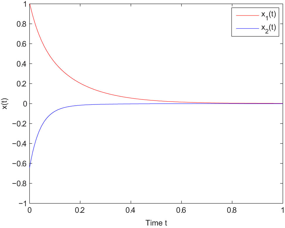
Asymptotic behavior in almost sure sense of the solution for equation (4.3).

5 Conclusions

The SDDEs driven by time-changed Brownian motions is a new research area for recent years. In this work, we have considered the asymptotic stability of the time-changed SDDEs with Markovian switching, by expanding the time-changed Itô formula and the time-changed semi-martingale convergence theorem. Our result generalizes that of SDDEs in the literature. Due to the more construction of SDDEs with time change than the usual SDDEs, our result is not a trivial generalization.

Acknowledgement

The authors would like to thank referee for valuable comments and careful reading, which leads to a great improvement of the article.

Funding information: This work was supported by the National Natural Science Foundation of China (11961037 and 11861040).
Conflict of interest: The authors declare that they have no competing interests.

References

[1] C. T. H. Baker and E. Buckwar , Exponential stability in p-th mean of solutions, and of convergent Euler-type solutions, of stochastic delay differential equations, J. Comput. Appl. Math. 184 (2005), no. 2, 404–427. 10.1016/j.cam.2005.01.018Search in Google Scholar

[2] X. Mao , Exponential Stability of Stochastic Differential Equations, Marcel Dekker, New York, 1994. Search in Google Scholar

[3] X. Mao , Stochastic Differential Equations and Applications, Horwood Publishing, UK, 2007. 10.1533/9780857099402Search in Google Scholar

[4] P. Protter , Stochastic Integration and Differential Equations, Springer-Verlag, Berlin Heidelberg, 2005. 10.1007/978-3-662-10061-5Search in Google Scholar

[5] D. Liu , G. Yang , and W. Zhang , The stability of neutral stochastic delay differential equations with Poisson jumps by fixed points, J. Comput. Appl. Math. 235 (2011), no. 10, 3115–3120. 10.1016/j.cam.2008.10.030Search in Google Scholar

[6] X. Mao , A note on the LaSalle-type theorem for stochastic differential delay equations, J. Math. Anal. Appl. 268 (2002), 125–142. 10.1006/jmaa.2001.7803Search in Google Scholar

[7] W. Zhu , J. Huang , X. Ruan , and Z. Zhao , Exponential stability of stochastic differential equation with mixed delay, J. Appl. Math. 2014 (2014), 187037. 10.1155/2014/187037Search in Google Scholar

[8] X. Mao , J. Lam , S. Xu , and H. Gao , Razumikhin method and exponential stability of hybrid stochastic delay interval systems, J. Math. Anal. Appl. 314 (2006), 45–66. 10.1016/j.jmaa.2005.03.056Search in Google Scholar

[9] B. Li , D. Li , and D. Xu , Stability analysis for impulsive stochastic delay differential equations with Markovian switching, J. Franklin Inst. 350 (2013), 1848–1864. 10.1016/j.jfranklin.2013.05.009Search in Google Scholar

[10] X. Mao and C. Yuan , Stochastic Differential Equations with Markovian Switching, Imperial College Press, London, 2006. 10.1142/p473Search in Google Scholar

[11] Y. Xu and Z. He , Exponential stability of neutral stochastic delay differential equations with Markovian switching, Appl. Math. Lett. 52 (2016), 64–73. 10.1016/j.aml.2015.08.019Search in Google Scholar

[12] C. Yuan and X. Mao , Robust stability and controllability of stochastic differential delay equations with Markovian switching, Automatica 40 (2004), no. 3, 343–354. 10.1016/j.automatica.2003.10.012Search in Google Scholar

[13] L. Chlebak , P. Garmirian , and Q. Wu , Sub-diffusion processes in Hilbert space and their associated stochastic differential equations and Fokker-Planck-Kolmogorov equations, arXiv:1610.00208v1 (2016). Search in Google Scholar

[14] J. Bertoin , Subordinators: Examples and applications , in: P. Bernard (ed.), Lectures on Probability Theory and Statistics, Lecture Notes in Mathematics , vol. 1717, Springer, Berlin, Heidelberg, 1999, pp. 1–91, https://doi.org/10.1007/978-3-540-48115-7_1 . 10.1007/978-3-540-48115-7_1Search in Google Scholar

[15] K. Kobayashi , Stochastic calculus for a time-changed semimartingale and the associated stochastic differential equations, J. Theoret. Probab. 24 (2011), 789–820. 10.1007/s10959-010-0320-9Search in Google Scholar

[16] Q. Wu , Stability analysis for a class of nonlinear time-changed systems, Cogent Math. 3 (2016), 1228273, https://doi.org/10.1080/23311835.2016.1228273 . 10.1080/23311835.2016.1228273Search in Google Scholar

[17] E. Nane and Y. Ni , Stability of the solution of stochastic differential equation driven by time-changed Lévy noise, Proc. Amer. Math. Soc. 145 (2017), no. 7, 3085–3104, https://doi.org/10.1090/proc/13447 .10.1090/proc/13447Search in Google Scholar

[18] E. Nane and Y. Ni , Path stability of stochastic differential equations driven by time-changed Lévy noises, ALEA, Lat. Am. J. Probab. Math. Stat. 15 (2018), 479–507, https://doi.org/10.30757/ALEA.v15-20 . 10.30757/ALEA.v15-20Search in Google Scholar

[19] X. Zhang and C. Yuan , Razumikhin-type theorem on time-changed stochastic functional differential equations with Markovian switching, Open Math. 17 (2019), 689–699, https://doi.org/10.1515/math-2019-0055 . 10.1515/math-2019-0055Search in Google Scholar

[20] M. Magdziarz , Path properties of subdiffusion – a martingale approach, Stoch. Models 26 (2010), no. 2, 256–271. 10.1080/15326341003756379Search in Google Scholar

[21] D. Xu , B. Li , S. Long , and L. Teng , Moment estimate and existence for solutions of stochastic functional differential equations, Nonlinear Anal. 108 (2014), 128–143. 10.1016/j.na.2014.05.004Search in Google Scholar

[22] S. Boyd , L. Ghaoui , E. Feron , and V. Balakrishnan , Linear Matrix Inequalities in System and Control Theory, SIAM Studies in Applied Mathematics, Philadelphia, 1994. 10.1137/1.9781611970777Search in Google Scholar

Received: 2020-08-26

Revised: 2021-03-04

Accepted: 2021-06-03

Published Online: 2021-07-23

This work is licensed under the Creative Commons Attribution 4.0 International License.

Articles in the same Issue

https://doi.org/10.1515/math-2021-0054

Keywords for this article

asymptotic stability; time-changed stochastic delay differential equations; time-changed Brownian motions; Markovian switching

Creative Commons

BY 4.0