SEMT valuation and strength of subdivided star of K 1,4
-
Salma Kanwal
 ,
Mariam Imtiaz
,
Mariam Imtiaz

Abstract
This study focuses on finding super edge-magic total (SEMT) labeling and deficiency of imbalanced fork and disjoint union of imbalanced fork with star, bistar and path; in addition, the SEMT strength for Imbalanced Fork is investigated.
1 Preliminaries
Labeling is a technique that allots labels to the components of a graph. Total labeling gives us both components (vertices and edges) labeled. A
If a graph G allows at least one SEMT labeling, then the smallest of the magic constants for all possible distinct SEMT labelings of G describes SEMT strength,
In [1], the notion of EMT deficiency was proposed, and Figueroa-Centeno et al. [4] continued it to SEMT graphs. For any graph G, the SEMT deficiency, signified as
where
In [4,5], Figueroa-Centeno et al. proposed a conjecture about the confined deficiencies of the forests. In [6], an assumption was made as a special case of a previous one that says, the deficiency of each two-tree forest is not more than 1. The results in [7,8,9,10,11,12,13,14,15,16,17,18,19,20,21,22] are found to be useful in the aspect of examined labeling here. For more review, see the recent survey of graph labelings by Gallian [23].
In this paper, we formulated the results on SEMT labeling and deficiency of forests consisting of imbalanced fork and disjoint union of imbalanced fork with star, bistar and path, respectively. The values of parameters of the star, bistar and path are totally dependent on the parameters involved in the imbalanced fork.
2 Main results
Definition 2.1
An imbalanced fork, represented as
A single new vertex
respectively.
Note 1. Another way of writing imbalanced fork
The following lemma is an elementary tool for proving graphs to be SEMT. It will be used as a base in each result presented in this work.
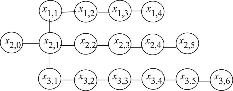
Imbalanced Fork
Lemma 2.2
[25] A
constructs
The following result of SEMT graphs also holds.
Note 2. [3] Let
For a single graph, many SEMT labelings might exist and of course for a different labeling, there will be a different magic constant. For lower and upper bounds of the magic constants for subdivided stars, see [26,27]. Now we are concerned with evaluating the SEMT labeling and strength of imbalanced fork.
Theorem 2.3
For
Proof
Let
Consider the vertex labeling
For
From the above labeling “f”, we obtain consecutive
For
From the above labeling “f”, we obtain consecutive
This theorem gives us the magic constants
Theorem 2.4
The SEMT strength for Imbalanced Fork
2.1 SEMT labeling and deficiency of forests formed by imbalanced fork, star, bistar and path
In this section, it is shown that the forests consisting of imbalanced fork, star, bistar and path are SEMT with certain conditions on the parameters.
Theorem 2.6
For
Proof
Consider the graph
Let
For
We define a labeling
Now consider the labeling
For
Let
From the above labeling “f”, we obtain consecutive
For
We define a labeling
Now consider the labeling
For
Let
From the above labeling “f”, we obtain consecutive
Let
Let
and
For
Keeping in mind the valuation f defined in (a), we describe the labeling
with
From the above labeling “
For
Keeping in mind the valuation f defined in (a), we describe the labeling
with
From the above labeling “
Theorem 2.7
For
Proof
Consider the graph
Let
For
Keeping in mind the valuation f defined in Theorem 2.6 with
From the above labeling “g”, we obtain consecutive
For
Keeping in mind the valuation f defined in Theorem 2.6 with
From the above labeling “g”, we obtain consecutive
Let
Here,
Let
and
For
with
From the above labeling “
For
with
From the above labeling “
In the following theorems, we present the two distinct SEMT labelings – which are non-dual of each other – for the same forest be composed of disjoint union of path
Theorem 2.8
For
(a)(i):
(a)(ii):
(b)(i):
(b)(ii):
Proof
Consider the graph
Let
For
Keeping in mind the valuation f defined in Theorem 2.6 with
From the above labeling “g”, we obtain consecutive
For
Keeping in mind the valuation f defined in Theorem 2.6 with
From the above labeling “g”, we obtain consecutive
Let
Let
where
For
Keeping in mind the valuation f defined in Theorem 2.6, we describe the labeling
with
Let
From the above labeling “
For
Keeping in mind the valuation f defined in Theorem 2.6, we describe the labeling
with
Let
From the above labeling “
Theorem 2.9
For
(a)(i):
(a)(ii):
(b)(i):
(b)(ii):
Proof
Consider the graph
Let
For
Keeping in mind the valuation f defined in Theorem 2.6 with
From the above labeling “g”, we obtain consecutive
For
Keeping in mind the valuation f defined in Theorem 2.6 with
From the above labeling “g′”, we obtain consecutive
Let
where
For
Keeping in mind the valuation f defined in Theorem 2.6, we describe the labeling
with
Let
From the above labeling “
For
Keeping in mind the valuation f defined in Theorem 2.6, we describe the labeling
with
Let
From the above labeling “
References
[1] A. Kotzig and A. Rosa, Magic valuations of finite graphs, Canad. Math. Bull. 13 (1970), 451–461.10.4153/CMB-1970-084-1Search in Google Scholar
[2] H. Enomoto, A. S. Lladó, T. Nakamigawa, and G. Ringel, Super edge-magic graphs, SUT J. Math. 34 (1998), no. 2, 105–109.10.55937/sut/991985322Search in Google Scholar
[3] S. Avadayappan, P. Jeyanthi, and R. Vasuki, Super magic strength of a graph, Indian J. Pure Appl. Math. 32 (2001), no. 11, 1621–1630.Search in Google Scholar
[4] R. M. Figueroa-Centeno, R. Ichishima, and F. A. Muntaner-Batle, On the super edge-magic deficiency of graphs, Ars Combin. 78 (2006), 33–45.10.1016/S1571-0653(04)00074-5Search in Google Scholar
[5] R. M. Figueroa-Centeno, R. Ichishima, and F. A. Muntaner-Batle, On the super edge-magic deficiency of graphs, Electron. Notes Discrete Math. 11 (2002), 299–314.10.1016/S1571-0653(04)00074-5Search in Google Scholar
[6] R. M. Figueroa-Centeno, R. Ichishima, and F. A. Muntaner-Batle, Some new results on the super edge-magic deficiency of graphs, J. Combin. Math. Combin. Comput. 55 (2005), 17–31.Search in Google Scholar
[7] A. A. Ngurah, E. T. Baskoro, and R. Simanjuntak, On the super edge-magic deficiencies of graphs, Australas. J. Combin. 40 (2008), 3–14.Search in Google Scholar
[8] S. Javed, A. Riasat, and S. Kanwal, On super edge magicness and deficiencies of forests, Utilitas Math. 98 (2015), 149–169.Search in Google Scholar
[9] K. Ali, M. Hussain, H. Shaker, and M. Javed, Super edge-magic total labeling of subdivided stars, Ars Combin. 120 (2015), 161–167.Search in Google Scholar
[10] V. Swamminatan and P. Jeyanthi, Super edge-magic strength of fire crackers, banana trees and unicyclic graphs, Discrete Math. 306 (2006), 1624–1636.10.1016/j.disc.2005.06.038Search in Google Scholar
[11] D. G. Akka and N. S. Warad, Super magic strength of a graph, Indian J. Pure Appl. Math. 41 (2010), no. 4, 557–568.10.1007/s13226-010-0031-zSearch in Google Scholar
[12] S. Kanwal, A. Azam, and Z. Iftikhar, SEMT labelings and deficiencies of forests with two components (II), Punjab Univ. J. Math. 51 (2019), no. 4, 1–12.Search in Google Scholar
[13] S. Kanwal, Z. Iftikhar, and A. Azam, SEMT labelings and deficiencies of forests with two components (I), Punjab Univ. J. Math. 51 (2019), no. 5, 137–149.Search in Google Scholar
[14] S. Kanwal, M. Imtiaz, Z. Iftikhar, R. Ashraf, M. Arshad, R. Irfan, and T. Sumbal, Embedding of supplementary results in strong EMT valuations and strength, Open Math. 17 (2019), no. 1, 527–543.10.1515/math-2019-0044Search in Google Scholar
[15] S. Kanwal and I. Kanwal, SEMT valuations of disjoint union of combs, stars and banana trees, Punjab Univ. J. Math. 50 (2018), no. 3, 131–144.Search in Google Scholar
[16] N. S. Hungund and D. G. Akka, Super edge-magic strength of some new families of graphs, Bull. Marathwada Math. Soc. 12 (2011), no. 1, 47–54.Search in Google Scholar
[17] M. Javaid and A. A. Bhatti, On super (a,d)-edge-antimagic total labeling of subdivided stars, Ars Combin. 105 (2012), 503–512.Search in Google Scholar
[18] M. Javed, M. Hassain, K. Ali, and H. Shaker, On super edge-magic total labeling on subdivision of trees, Util. Math. 89 (2012), 169–177.Search in Google Scholar
[19] A. Ali, M. Javaid, and M. A. Rehman, SEMT labeling on disjoint union of subdivided stars, Punjab Uni. J. Math. 48 (2016), no. 1, 111–122.Search in Google Scholar
[20] V. Swaminathan and P. Jeyanthi, Super edge-magic strength of generalised theta graphs, Int. J. Inf. Manag. Sci. 22 (2006), no. 3, 203–220.Search in Google Scholar
[21] V. Swaminathan and P. Jeyanthi, Strong super edge-magic graphs, Math. Educ. XLII (2008), no. 3, 156–160.Search in Google Scholar
[22] V. Swaminathan and P. Jeyanthi, Super edge-magic labeling of some new classes of graphs, Math. Educ. XLII (2008), no. 2, 91–94.Search in Google Scholar
[23] J. A. Gallian, A dynamic survey of graph labeling, 22th edition, Electron. J. Combin. (Dec. 2019), # DS6.Search in Google Scholar
[24] S. Kanwal, A. Riasat, M. Imtiaz, Z. Iftikhar, S. Javed, and R. Ashraf, Bounds of strong EMT strength for certain subdivision of star and bistar, Open Math. 16 (2018), 1313–1325.10.1515/math-2018-0111Search in Google Scholar
[25] R. M. Figueroa-Centeno, R. Ichishima, and F. A. Muntaner-Batle, The place of super edge-magic labeling among other classes of labeling, Discrete Math. 231 (2001), 153–168.10.1016/S0012-365X(00)00314-9Search in Google Scholar
[26] E. T. Baskoro, A. A. G. Ngurah, and R. Simanjuntak, On (super) edge-magic total labeling of subdivision of K1,3, SUT J. Math. 43 (2007), 127–136.10.55937/sut/1252506095Search in Google Scholar
[27] M. Javaid, Labeling Graphs and Hypergraphs, PhD thesis, FAST-NUCES, Lahore Campus, Pakistan, 2013.Search in Google Scholar
© 2020 Salma Kanwal et al., published by De Gruyter
This work is licensed under the Creative Commons Attribution 4.0 International License.
Articles in the same Issue
- Regular Articles
- Non-occurrence of the Lavrentiev phenomenon for a class of convex nonautonomous Lagrangians
- Strong and weak convergence of Ishikawa iterations for best proximity pairs
- Curve and surface construction based on the generalized toric-Bernstein basis functions
- The non-negative spectrum of a digraph
- Bounds on F-index of tricyclic graphs with fixed pendant vertices
- Crank-Nicolson orthogonal spline collocation method combined with WSGI difference scheme for the two-dimensional time-fractional diffusion-wave equation
- Hardy’s inequalities and integral operators on Herz-Morrey spaces
- The 2-pebbling property of squares of paths and Graham’s conjecture
- Existence conditions for periodic solutions of second-order neutral delay differential equations with piecewise constant arguments
- Orthogonal polynomials for exponential weights x2α(1 – x2)2ρe–2Q(x) on [0, 1)
- Rough sets based on fuzzy ideals in distributive lattices
- On more general forms of proportional fractional operators
- The hyperbolic polygons of type (ϵ, n) and Möbius transformations
- Tripled best proximity point in complete metric spaces
- Metric completions, the Heine-Borel property, and approachability
- Functional identities on upper triangular matrix rings
- Uniqueness on entire functions and their nth order exact differences with two shared values
- The adaptive finite element method for the Steklov eigenvalue problem in inverse scattering
- Existence of a common solution to systems of integral equations via fixed point results
- Fixed point results for multivalued mappings of Ćirić type via F-contractions on quasi metric spaces
- Some inequalities on the spectral radius of nonnegative tensors
- Some results in cone metric spaces with applications in homotopy theory
- On the Malcev products of some classes of epigroups, I
- Self-injectivity of semigroup algebras
- Cauchy matrix and Liouville formula of quaternion impulsive dynamic equations on time scales
- On the symmetrized s-divergence
- On multivalued Suzuki-type θ-contractions and related applications
- Approximation operators based on preconcepts
- Two types of hypergeometric degenerate Cauchy numbers
- The molecular characterization of anisotropic Herz-type Hardy spaces with two variable exponents
- Discussions on the almost 𝒵-contraction
- On a predator-prey system interaction under fluctuating water level with nonselective harvesting
- On split involutive regular BiHom-Lie superalgebras
- Weighted CBMO estimates for commutators of matrix Hausdorff operator on the Heisenberg group
- Inverse Sturm-Liouville problem with analytical functions in the boundary condition
- The L-ordered L-semihypergroups
- Global structure of sign-changing solutions for discrete Dirichlet problems
- Analysis of F-contractions in function weighted metric spaces with an application
- On finite dual Cayley graphs
- Left and right inverse eigenpairs problem with a submatrix constraint for the generalized centrosymmetric matrix
- Controllability of fractional stochastic evolution equations with nonlocal conditions and noncompact semigroups
- Levinson-type inequalities via new Green functions and Montgomery identity
- The core inverse and constrained matrix approximation problem
- A pair of equations in unlike powers of primes and powers of 2
- Miscellaneous equalities for idempotent matrices with applications
- B-maximal commutators, commutators of B-singular integral operators and B-Riesz potentials on B-Morrey spaces
- Rate of convergence of uniform transport processes to a Brownian sheet
- Curves in the Lorentz-Minkowski plane with curvature depending on their position
- Sequential change-point detection in a multinomial logistic regression model
- Tiny zero-sum sequences over some special groups
- A boundedness result for Marcinkiewicz integral operator
- On a functional equation that has the quadratic-multiplicative property
- The spectrum generated by s-numbers and pre-quasi normed Orlicz-Cesáro mean sequence spaces
- Positive coincidence points for a class of nonlinear operators and their applications to matrix equations
- Asymptotic relations for the products of elements of some positive sequences
- Jordan {g,h}-derivations on triangular algebras
- A systolic inequality with remainder in the real projective plane
- A new characterization of L2(p2)
- Nonlinear boundary value problems for mixed-type fractional equations and Ulam-Hyers stability
- Asymptotic normality and mean consistency of LS estimators in the errors-in-variables model with dependent errors
- Some non-commuting solutions of the Yang-Baxter-like matrix equation
- General (p,q)-mixed projection bodies
- An extension of the method of brackets. Part 2
- A new approach in the context of ordered incomplete partial b-metric spaces
- Sharper existence and uniqueness results for solutions to fourth-order boundary value problems and elastic beam analysis
- Remark on subgroup intersection graph of finite abelian groups
- Detectable sensation of a stochastic smoking model
- Almost Kenmotsu 3-h-manifolds with transversely Killing-type Ricci operators
- Some inequalities for star duality of the radial Blaschke-Minkowski homomorphisms
- Results on nonlocal stochastic integro-differential equations driven by a fractional Brownian motion
- On surrounding quasi-contractions on non-triangular metric spaces
- SEMT valuation and strength of subdivided star of K 1,4
- Weak solutions and optimal controls of stochastic fractional reaction-diffusion systems
- Gradient estimates for a weighted nonlinear parabolic equation and applications
- On the equivalence of three-dimensional differential systems
- Free nonunitary Rota-Baxter family algebras and typed leaf-spaced decorated planar rooted forests
- The prime and maximal spectra and the reticulation of residuated lattices with applications to De Morgan residuated lattices
- Explicit determinantal formula for a class of banded matrices
- Dynamics of a diffusive delayed competition and cooperation system
- Error term of the mean value theorem for binary Egyptian fractions
- The integral part of a nonlinear form with a square, a cube and a biquadrate
- Meromorphic solutions of certain nonlinear difference equations
- Characterizations for the potential operators on Carleson curves in local generalized Morrey spaces
- Some integral curves with a new frame
- Meromorphic exact solutions of the (2 + 1)-dimensional generalized Calogero-Bogoyavlenskii-Schiff equation
- Towards a homological generalization of the direct summand theorem
- A standard form in (some) free fields: How to construct minimal linear representations
- On the determination of the number of positive and negative polynomial zeros and their isolation
- Perturbation of the one-dimensional time-independent Schrödinger equation with a rectangular potential barrier
- Simply connected topological spaces of weighted composition operators
- Generalized derivatives and optimization problems for n-dimensional fuzzy-number-valued functions
- A study of uniformities on the space of uniformly continuous mappings
- The strong nil-cleanness of semigroup rings
- On an equivalence between regular ordered Γ-semigroups and regular ordered semigroups
- Evolution of the first eigenvalue of the Laplace operator and the p-Laplace operator under a forced mean curvature flow
- Noetherian properties in composite generalized power series rings
- Inequalities for the generalized trigonometric and hyperbolic functions
- Blow-up analyses in nonlocal reaction diffusion equations with time-dependent coefficients under Neumann boundary conditions
- A new characterization of a proper type B semigroup
- Constructions of pseudorandom binary lattices using cyclotomic classes in finite fields
- Estimates of entropy numbers in probabilistic setting
- Ramsey numbers of partial order graphs (comparability graphs) and implications in ring theory
- S-shaped connected component of positive solutions for second-order discrete Neumann boundary value problems
- The logarithmic mean of two convex functionals
- A modified Tikhonov regularization method based on Hermite expansion for solving the Cauchy problem of the Laplace equation
- Approximation properties of tensor norms and operator ideals for Banach spaces
- A multi-power and multi-splitting inner-outer iteration for PageRank computation
- The edge-regular complete maps
- Ramanujan’s function k(τ)=r(τ)r2(2τ) and its modularity
- Finite groups with some weakly pronormal subgroups
- A new refinement of Jensen’s inequality with applications in information theory
- Skew-symmetric and essentially unitary operators via Berezin symbols
- The limit Riemann solutions to nonisentropic Chaplygin Euler equations
- On singularities of real algebraic sets and applications to kinematics
- Results on analytic functions defined by Laplace-Stieltjes transforms with perfect ϕ-type
- New (p, q)-estimates for different types of integral inequalities via (α, m)-convex mappings
- Boundary value problems of Hilfer-type fractional integro-differential equations and inclusions with nonlocal integro-multipoint boundary conditions
- Boundary layer analysis for a 2-D Keller-Segel model
- On some extensions of Gauss’ work and applications
- A study on strongly convex hyper S-subposets in hyper S-posets
- On the Gevrey ultradifferentiability of weak solutions of an abstract evolution equation with a scalar type spectral operator on the real axis
- Special Issue on Graph Theory (GWGT 2019), Part II
- On applications of bipartite graph associated with algebraic structures
- Further new results on strong resolving partitions for graphs
- The second out-neighborhood for local tournaments
- On the N-spectrum of oriented graphs
- The H-force sets of the graphs satisfying the condition of Ore’s theorem
- Bipartite graphs with close domination and k-domination numbers
- On the sandpile model of modified wheels II
- Connected even factors in k-tree
- On triangular matroids induced by n3-configurations
- The domination number of round digraphs
- Special Issue on Variational/Hemivariational Inequalities
- A new blow-up criterion for the N – abc family of Camassa-Holm type equation with both dissipation and dispersion
- On the finite approximate controllability for Hilfer fractional evolution systems with nonlocal conditions
- On the well-posedness of differential quasi-variational-hemivariational inequalities
- An efficient approach for the numerical solution of fifth-order KdV equations
- Generalized fractional integral inequalities of Hermite-Hadamard-type for a convex function
- Karush-Kuhn-Tucker optimality conditions for a class of robust optimization problems with an interval-valued objective function
- An equivalent quasinorm for the Lipschitz space of noncommutative martingales
- Optimal control of a viscous generalized θ-type dispersive equation with weak dissipation
- Special Issue on Problems, Methods and Applications of Nonlinear analysis
- Generalized Picone inequalities and their applications to (p,q)-Laplace equations
- Positive solutions for parametric (p(z),q(z))-equations
- Revisiting the sub- and super-solution method for the classical radial solutions of the mean curvature equation
- (p,Q) systems with critical singular exponential nonlinearities in the Heisenberg group
- Quasilinear Dirichlet problems with competing operators and convection
- Hyers-Ulam-Rassias stability of (m, n)-Jordan derivations
- Special Issue on Evolution Equations, Theory and Applications
- Instantaneous blow-up of solutions to the Cauchy problem for the fractional Khokhlov-Zabolotskaya equation
- Three classes of decomposable distributions