Explicit order 3/2 Runge-Kutta method for numerical solutions of stochastic differential equations by using Itô-Taylor expansion
-
Yazid Alhojilan


Abstract
This paper aims to present a new pathwise approximation method, which gives approximate solutions of order
1 Introduction
The purpose of this paper is to develop a new pathwise approximation to numerical solutions of SDEs driven by multidimensional Brownian motion. There is a standard approach, which described in [1], approximates solutions of SDEs to the required order using stochastic Taylor expansion at each time step. Nevertheless, applying this method would be difficult when the deriving Brownian motion dimension is greater than 1 to get higher order than
In this paper, we aim to present a new pathwise approximation scheme that can be used to get a higher-order approximation for Brownian motion in dimension greater than 1. It is based on using a coupling and a version of the perturbation method. Therefore, this new scheme does not require calculating Iα, because we replace them by random variables with the same moments conditional on the linear term. Then, we get a random vector, which is a good approximation in distribution to the original Taylor expansion, and it can be generated using algorithms in MATLAB. We have used a technique from optimal transport theory [5] to give a good approximation in mean square. Other works use a coupling to approximate SDEs numerically, such that [6, 7, 8, 9]. This paper, organized as follows: section 2, gives a background material, and section 3, shows the implementation of the scheme.
2 Background
Let (Ω, 𝓕, P) be a probability space. Let σ(x̂s : s ≤ t) denote the smallest σ-algebra such that x̂s (a stochastic process) is σ(x̂s : s ≤ t)-measurable for all s ≤ t. A collection of σ-algebras {𝓕t}, satisfying (i.e. 𝓕t ⊂ 𝓕s ⊂ 𝓕 for all 0 ≤ t < s < ∞) is called a filtration. 𝓕t is interpreted as corresponding to the information available at time t (the amount of information increasing as time progresses). A stochastic process x̂t is adapted to a filtration {𝓕t} if x̂t is 𝓕t-measurable for all t ≥ 0.
2.1 Stochastic Itô-Taylor expansion
Let us consider a 1-dimensional Ito stochastic differential equation in the form of an integral
where a(t, x) and b(t, x) are Borel measurable functions defined on [0, ∞) × ℝ) with values in ℝ. Hence, for f : 𝓡 → 𝓡 which is a twice continuously differentiable function, the Itô formula [1] gives
where the operators are
and
Clearly, if f(x) ≡ x we have L0f = a and L1f = b, in which case that there is a reduction in (2.2) to the original Itô equation for x̂t, that is to
Applying the Itô formula (2.2) to the function f = a and f = b in (2.5), we obtain
where the remainder is
For the Taylor expansion of d-dimensional Itô stochastic differential equations, a similar expansion holds as above for
The general Itô Taylor expansion is given in (2.12).
2.2 Perturbation method
Consider the following: suppose we wish to simulate U = X + ϵ Y, where X and Y are independent, X has a smooth density, and ϵ is small. Also, suppose that X is easy to generate, while Y is hard to generate. Then, generating U by generating X and Y will be hard. Alternatively, let us suppose there is another random variable that is easy to generate to overcome this dilemma, say Z, which is independent of X. The random variable Z has the same moments up to order m − 1 as Y (i.e. E(Zk) = E(Yk) for k = 1, 2, 3, …, m − 1). Then, we can prove that V = X + ϵ Z is an approximation to U with the error of order ϵm. The justification for this can be seen by writing fX for the density of X etc, so we have fU(x) = EfX(x − ϵ Y) = f(x) +
2.3 Construction of pathwise approximation of SDEs using stochastic Taylor expansions
Consider an Itô SDE
on an interval [0, T], for a q-dimensional vector x̂t, with a d-dimensional driving Brownian path Wt. Assume (2.9) satisfies an existence and uniqueness theorem. The basic idea to get pathwise approximation is to divide [0, T] into a finite number N of subintervals, where the length of the step equals h =
The basic scheme which we have is Euler-Maruyama
In order to get the Milstein scheme, we add the quadratic terms
where
Our constructed method, which approximates SDEs at order
For m ≥ 2 in ℕ we define
where n(α) is the number of zero indices in α.
The case l(α) = n(α) =
where ℝq-valued functions fα,i(t, x̂) are defined recursively by fv(t, x̂) = x̂ and fjα = Lj fα for j ∈ {0, …, d}, where v is the multi-index of zero length, and fα,i denotes the ith component of fα.
The main point which will be discussed in this paper; how do we generate RHS of (2.12) easily? Actually, this research has developed a scheme where to generate RHS of (2.12) by using perturbation and coupling method; how?
Let us apply this method in (2.12) in order to approximate SDEs at higher order. In order to simplify application, we will be deal with the first iteration from 0 to h of (2.12)
where
for i = 1, …, q, where bik(0, x̂(0)) and fα,i(0, x̂(0)) are real constants.
As Iα is not independent of Δ W, so it would be difficult to generate these stochastic integrals when we want to find approximate solutions. By following the construction in [10], we can overcome this issue using the relation
For α = (j1, …, jl) we can replace the iterated stochastic integrals Iα using random variables with the same moments conditional on the linear term as follows
where we calculate the sum over all β = (i1, …, il) such that for each k ∈ {1, …, l} we have either ik = jk or ik = 0 < jk. (For examples I013 = h2(K013 + K003 V1 + K010 V3 + K000 V1 V3)). The random variables Kβ and Vk ∼ N(0, 1) are generated independently.
By setting
where Vk is independent N(0, 1) of a random variable Kα and Qi is a polynomial, each monomial of which has overall order at least 2 in ϵ.
We have found it hard to generate Y directly by using (2.14). To tackle this problem, we use a version of the perturbation method by assuming random variables Lβ and using them rather than Kβ which easy to generate for α ∈ 𝓜 such that 2 ≤ l(α) ≤ m.
It will be discussed the way of construction Lβ later in this section with details.
Then, (2.14) can be modified as follows
where we calculate the sum over all β = (i1, …, il) such that for each k ∈ {1, …, l} we have either ik = jk or ik = 0 < jk. (For example Ī013 = h2 (L013 + L003 V̄1 + L010 V̄3 + L000 V̄1 V̄3)). The random variables Lβ and V̄k ∼ N(0, 1) are generated independently.
Then, we can be redefine the formula (2.5) as follows
where V̄k are independent N(0, 1) and independent of the random variable Lα.
The following theorem is essential to give the error bound in the approximation by the modified Y by considering equation (2.9) and using the notation of section (2.12).
Theorem 1
This theorem is Lp version of [10].
Assume the matrix (bik) has rank q. Suppose the random variables Lα have all moments finite and that 𝔼(Kα1 … Kαr) = 𝔼(Lα1 … Lαr) whenever α1, …, αr ∈ 𝓜m satisfy
Proof
We refer the reader to [11]. □
How do we apply theorem 1 to generate approximate solution for (2.12)?
Basically, we assume coefficients ak and bik are sufficiently regular (uniform bounds for the coefficients and their derivatives up to order two will certainly suffice) and the matrix (bik) has rank q everywhere with uniformly bounded right inverse. Then, the iterated integrals Iα,jh,(j+1)h in (2.12) are hard to generate as it has been mentioned so we should use modification of iterated integrals which are easy to generate Īα,jh,(j+1)h [10]. The modified formula which results is the following
We now return to think about the application of coupling to the simulations of SDEs in the first step between Y and Ȳ. We have assumed the Lβ satisfy the hypothesis of the theorem 1 such that 𝔼(Kα1 … Kαr) = 𝔼(Lα1 … Lαr) whenever α1, …, αr ∈ 𝓜m satisfy
For the bound at j step, we can use the same argument as used in (2.19) to deduce the bound for (2.21), except that the coefficient functions evaluated at random variables
Therefore, by nested expectation, we have
It is required to know the calculations of the relevant expectation of products of Kβ for generating a suitable random variables Lβ. However, before doing that, we would clarify how to construct proper random variables. First, the new random variables Lβ must satisfy the moment conditions in the statement of theorem 1. Thus, once the relevant moments of the Kβ are calculated, then it would be taken any choice of Lβ which satisfies these moment conditions of the theorem 1. To calculate the moments, we have used the following three lemmas.
Lemma 1
[10]. Let β = (j j … j) with length l ≥ 2. Then (i) if j = 0 then Kβ =
Lemma 2
[10]. If β1, …, βs ∈ 𝓜 and if some j ≥ 1 occurs an odd number of times in the concatenated multi-index β1 … βs then 𝔼(Kβ1 … Kβs) = 0.
Lemma 3
[10]. (i) if 0 ≤ k < l then Klk = −Kkl and
Klk = −Kkl can be proved by using integration by parts as follows
3 Implementation of the method
In the preceding section, it has introduced the method that can be used to get approximate solutions of higher-order for any dimension of Brownian motions. Therefore, to get numerical solutions for SDEs of order
For β in the definition of Īα in (2.16), we need all indices of length 2 and 3. The random variables Lβ in (2.16) must satisfy the moment condition in the statement of theorem 1, that 𝔼(Kα1 … Kαr) = 𝔼(Lα1 … Lαr) whenever α1, …, αr ∈ 𝓜m satisfy
Deterministic Kα
K00 =
Kkk = −
Non-deterministic moments
Klk = −Kkl, for 0 ≤ k < l,
𝔼(Kkl) = 0, for 0 ≤ k < l,
𝔼(Knkl) = 0, for k, l, n > 0,
𝔼(K0kk) = 𝔼(Kk0k) = 𝔼(Kkk0) = −
𝔼(Kα) = 0 if α = 0kl or a permutation of it for k < l and k, l > 0,
𝔼(Kα) = 0 if α = 00l or a permutation of it for l > 0,
𝔼(Kkl Kk1l1) = 0, for k < l, k1 < l1 and kl ≠ k1l1,
3.1 Construction of Lβ
In this section, we discuss the choices that we make for Lα. Firstly, for all the deterministic α, the random variables Lα have the same values as 𝔼(Kα). For α of length 3, we only need the expectations, so we can choose them to be deterministic by making them equal to 𝔼(Kα). For the cases of the products, we can use the fact of the antisymmetry Klk = −Kkl for k < l, so we choose the random variables Llk with k < l which satisfy it. Therefore, the expectations for the products (Lα Lβ) (α and β are distinct and not deterministic) are zeros such as 𝔼(LlkLl1k1) = 0 for k < l, k1 < l1 and k, l ≠ k1, l1.
Hence, the random variables Lkl with k < l are required to have all moments finite, mean zero, variance
As a result, we set Llk = −Lkl for 0 ≤ k < 1, and by using lemma 1, 2 and 3, they give L00 =
for k, l, n > 0.
3.2 Completion of the method
The following calculation is for finding fα,i. The definitions of the Itô diffusion operators L0 (2.3) and Lj (2.4) are used to determine the fα,i.
Combining these in (2.18), it gives us the following formula
where for each j the random variables
where
3.3 Simulation result
The following system of SDEs had simulated by using (3.4) for the number of steps N = 200.
Figure 1 shows the piecewise linear curve through the values for the approximate solutions at each time step.
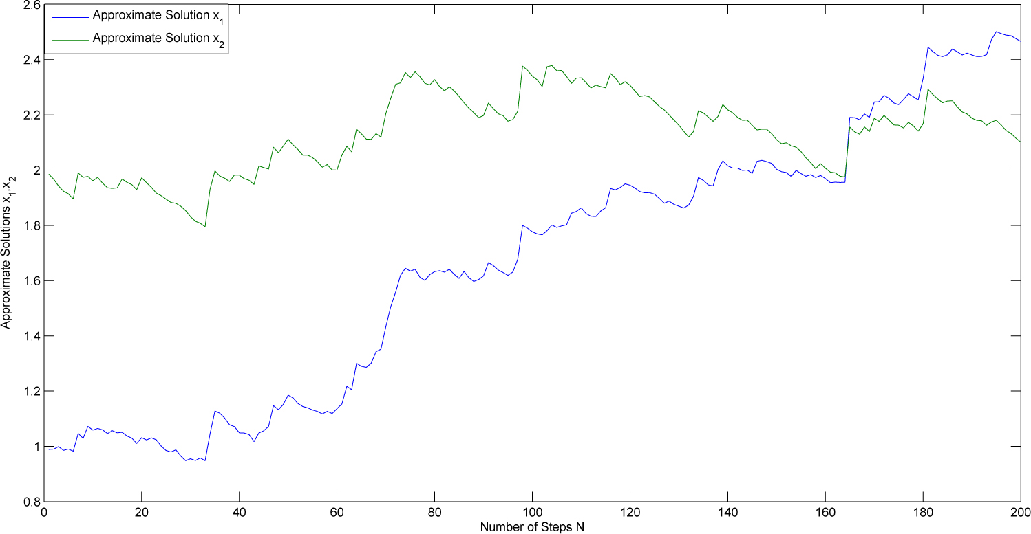
Approximate solutions of (3.7).
In Table 1, we calculate the error of the method at a time interval [0, T], where T = 1 by using the iteration numbers N = 5, 10 and 20, step sizes h = 1/5, 1/10 and 1/20 and the simulation number R = 4000000.
Mean squared error.
| N | Mean squared error E | Confidence intervals |
|---|---|---|
| 5 | 0.0184 | 0.0146:0.0222 |
| 10 | 0.0050 | 0.0012:0.0088 |
| 20 | 0.0015 | −0.0023:0.0058 |
Figure 2 shows the confidence intervals along the line of the least square for the expectations against step sizes. The blue line is the least square. The level of the confidence interval is 95%. The green line is the upper confidence bounds, while the red line is the lower confidence bounds. The red line has just two points because the lower bound of one of the confidence intervals is negative. Therefore, we swap the negative value in the confidence interval with the zero, so when we take the log for this confidence interval, then we get −∞ as the lower bound for this confidence interval, but it does not show in the graph. Therefore, we have used this method to handle the negative value in the confidence interval because if we do not do this, then the least square regression line does not pass through confidence intervals as it should be. This scheme aims to give approximation at order
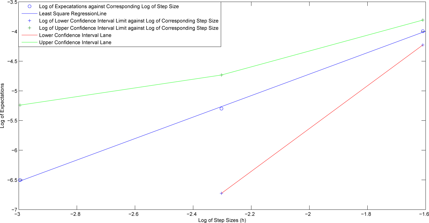
Convergence of the method.
4 Conclusion
The paper presents a numerical method that gives approximate solutions of stochastic differential equations with a strong error rate of
Acknowledgment
The author would like to thank Prof. Davie and Prof. Gyongy from Edinburgh University for many useful discussions, especially Prof. Davie, who answering many questions. The author is grateful for the support of Qassim University and Edinburgh University.
References
[1] Kloeden P.E., Platen E., Numerical Solution of Stochastic Differential Equations, Springer-Verlag Berlin Heidelberg New York, 1995.Search in Google Scholar
[2] Gaines J.G., Lyons T.J., Random generation of stochastic area integrals, SIAM J.Appl. Math., 1994, 54, 1132–1146.10.1137/S0036139992235706Search in Google Scholar
[3] Rydén T., Wiktorsson M., On the simulation of iterated Itô integrals, Stochastic Processes Appl, 2001, 91, 151–168.10.1016/S0304-4149(00)00053-3Search in Google Scholar
[4] Wiktorsson M., Joint characteristic function and simultaneous simulation of iterated Itô integrals for multiple independent Brownian motions, Ann. Appl. Probab., 2001, 11, 470–487.10.1214/aoap/1015345301Search in Google Scholar
[5] Villani C., Topics in Optimal Transportation, American Mathematical Society, 2003.10.1090/gsm/058Search in Google Scholar
[6] Alfonsi A., Jourdain B., Kohatsu-Higa A., Pathwise optimal transport bounds between a one-dimensional diffusion and its Euler scheme, Ann. Appl. Probab., 2014, 24, 1049–1080.10.1214/13-AAP941Search in Google Scholar
[7] Rio E., Upper bounds for minimal distances in the central limit theorem, Ann. Inst. Henri Poincar’e Probab. Stat., 2009, 45, 802–817.10.1214/08-AIHP187Search in Google Scholar
[8] Komlós J., Major P., Tusnády G., An approximation of partial sums of independent RV's and the sample DF. I, Z. Wahr. und Wer. Gebiete, 1975, 32, 111–131.10.1007/BF00533093Search in Google Scholar
[9] Rachev S.T., Ruschendorff L., Mass transportation problems, Volume 1, Theory; Volume 2, Applications, Springer-Verlag Berlin Heidelberg New York, 1998.Search in Google Scholar
[10] Davie A.M., Pathwise approximation of stochastic differential equations using coupling, http://www.maths.ed.ac.uk/∼sandy/coum.pdf.Search in Google Scholar
[11] Davie A.M., Polynomial perturbations of normal distributions, www.maths.ed.ac.uk/∼adavie/polg.pdf.Search in Google Scholar
[12] Gaines J.G., The algebra of iterated stochastic integrals, Stochastics and Stochastics Reports, 1993, 49, 169–179.10.1080/17442509408833918Search in Google Scholar
© 2019 Yazid Alhojilan, published by De Gruyter
This work is licensed under the Creative Commons Attribution 4.0 Public License.
Articles in the same Issue
- Regular Articles
- On the Gevrey ultradifferentiability of weak solutions of an abstract evolution equation with a scalar type spectral operator of orders less than one
- Centralizers of automorphisms permuting free generators
- Extreme points and support points of conformal mappings
- Arithmetical properties of double Möbius-Bernoulli numbers
- The product of quasi-ideal refined generalised quasi-adequate transversals
- Characterizations of the Solution Sets of Generalized Convex Fuzzy Optimization Problem
- Augmented, free and tensor generalized digroups
- Time-dependent attractor of wave equations with nonlinear damping and linear memory
- A new smoothing method for solving nonlinear complementarity problems
- Almost periodic solution of a discrete competitive system with delays and feedback controls
- On a problem of Hasse and Ramachandra
- Hopf bifurcation and stability in a Beddington-DeAngelis predator-prey model with stage structure for predator and time delay incorporating prey refuge
- A note on the formulas for the Drazin inverse of the sum of two matrices
- Completeness theorem for probability models with finitely many valued measure
- Periodic solution for ϕ-Laplacian neutral differential equation
- Asymptotic orbital shadowing property for diffeomorphisms
- Modular equations of a continued fraction of order six
- Solutions with concentration and cavitation to the Riemann problem for the isentropic relativistic Euler system for the extended Chaplygin gas
- Stability Problems and Analytical Integration for the Clebsch’s System
- Topological Indices of Para-line Graphs of V-Phenylenic Nanostructures
- On split Lie color triple systems
- Triangular Surface Patch Based on Bivariate Meyer-König-Zeller Operator
- Generators for maximal subgroups of Conway group Co1
- Positivity preserving operator splitting nonstandard finite difference methods for SEIR reaction diffusion model
- Characterizations of Convex spaces and Anti-matroids via Derived Operators
- On Partitions and Arf Semigroups
- Arithmetic properties for Andrews’ (48,6)- and (48,18)-singular overpartitions
- A concise proof to the spectral and nuclear norm bounds through tensor partitions
- A categorical approach to abstract convex spaces and interval spaces
- Dynamics of two-species delayed competitive stage-structured model described by differential-difference equations
- Parity results for broken 11-diamond partitions
- A new fourth power mean of two-term exponential sums
- The new operations on complete ideals
- Soft covering based rough graphs and corresponding decision making
- Complete convergence for arrays of ratios of order statistics
- Sufficient and necessary conditions of convergence for ρ͠ mixing random variables
- Attractors of dynamical systems in locally compact spaces
- Random attractors for stochastic retarded strongly damped wave equations with additive noise on bounded domains
- Statistical approximation properties of λ-Bernstein operators based on q-integers
- An investigation of fractional Bagley-Torvik equation
- Pentavalent arc-transitive Cayley graphs on Frobenius groups with soluble vertex stabilizer
- On the hybrid power mean of two kind different trigonometric sums
- Embedding of Supplementary Results in Strong EMT Valuations and Strength
- On Diophantine approximation by unlike powers of primes
- A General Version of the Nullstellensatz for Arbitrary Fields
- A new representation of α-openness, α-continuity, α-irresoluteness, and α-compactness in L-fuzzy pretopological spaces
- Random Polygons and Estimations of π
- The optimal pebbling of spindle graphs
- MBJ-neutrosophic ideals of BCK/BCI-algebras
- A note on the structure of a finite group G having a subgroup H maximal in 〈H, Hg〉
- A fuzzy multi-objective linear programming with interval-typed triangular fuzzy numbers
- Variational-like inequalities for n-dimensional fuzzy-vector-valued functions and fuzzy optimization
- Stability property of the prey free equilibrium point
- Rayleigh-Ritz Majorization Error Bounds for the Linear Response Eigenvalue Problem
- Hyper-Wiener indices of polyphenyl chains and polyphenyl spiders
- Razumikhin-type theorem on time-changed stochastic functional differential equations with Markovian switching
- Fixed Points of Meromorphic Functions and Their Higher Order Differences and Shifts
- Properties and Inference for a New Class of Generalized Rayleigh Distributions with an Application
- Nonfragile observer-based guaranteed cost finite-time control of discrete-time positive impulsive switched systems
- Empirical likelihood confidence regions of the parameters in a partially single-index varying-coefficient model
- Algebraic loop structures on algebra comultiplications
- Two weight estimates for a class of (p, q) type sublinear operators and their commutators
- Dynamic of a nonautonomous two-species impulsive competitive system with infinite delays
- 2-closures of primitive permutation groups of holomorph type
- Monotonicity properties and inequalities related to generalized Grötzsch ring functions
- Variation inequalities related to Schrödinger operators on weighted Morrey spaces
- Research on cooperation strategy between government and green supply chain based on differential game
- Extinction of a two species competitive stage-structured system with the effect of toxic substance and harvesting
- *-Ricci soliton on (κ, μ)′-almost Kenmotsu manifolds
- Some improved bounds on two energy-like invariants of some derived graphs
- Pricing under dynamic risk measures
- Finite groups with star-free noncyclic graphs
- A degree approach to relationship among fuzzy convex structures, fuzzy closure systems and fuzzy Alexandrov topologies
- S-shaped connected component of radial positive solutions for a prescribed mean curvature problem in an annular domain
- On Diophantine equations involving Lucas sequences
- A new way to represent functions as series
- Stability and Hopf bifurcation periodic orbits in delay coupled Lotka-Volterra ring system
- Some remarks on a pair of seemingly unrelated regression models
- Lyapunov stable homoclinic classes for smooth vector fields
- Stabilizers in EQ-algebras
- The properties of solutions for several types of Painlevé equations concerning fixed-points, zeros and poles
- Spectrum perturbations of compact operators in a Banach space
- The non-commuting graph of a non-central hypergroup
- Lie symmetry analysis and conservation law for the equation arising from higher order Broer-Kaup equation
- Positive solutions of the discrete Dirichlet problem involving the mean curvature operator
- Dislocated quasi cone b-metric space over Banach algebra and contraction principles with application to functional equations
- On the Gevrey ultradifferentiability of weak solutions of an abstract evolution equation with a scalar type spectral operator on the open semi-axis
- Differential polynomials of L-functions with truncated shared values
- Exclusion sets in the S-type eigenvalue localization sets for tensors
- Continuous linear operators on Orlicz-Bochner spaces
- Non-trivial solutions for Schrödinger-Poisson systems involving critical nonlocal term and potential vanishing at infinity
- Characterizations of Benson proper efficiency of set-valued optimization in real linear spaces
- A quantitative obstruction to collapsing surfaces
- Dynamic behaviors of a Lotka-Volterra type predator-prey system with Allee effect on the predator species and density dependent birth rate on the prey species
- Coexistence for a kind of stochastic three-species competitive models
- Algebraic and qualitative remarks about the family yy′ = (αxm+k–1 + βxm–k–1)y + γx2m–2k–1
- On the two-term exponential sums and character sums of polynomials
- F-biharmonic maps into general Riemannian manifolds
- Embeddings of harmonic mixed norm spaces on smoothly bounded domains in ℝn
- Asymptotic behavior for non-autonomous stochastic plate equation on unbounded domains
- Power graphs and exchange property for resolving sets
- On nearly Hurewicz spaces
- Least eigenvalue of the connected graphs whose complements are cacti
- Determinants of two kinds of matrices whose elements involve sine functions
- A characterization of translational hulls of a strongly right type B semigroup
- Common fixed point results for two families of multivalued A–dominated contractive mappings on closed ball with applications
- Lp estimates for maximal functions along surfaces of revolution on product spaces
- Path-induced closure operators on graphs for defining digital Jordan surfaces
- Irreducible modules with highest weight vectors over modular Witt and special Lie superalgebras
- Existence of periodic solutions with prescribed minimal period of a 2nth-order discrete system
- Injective hulls of many-sorted ordered algebras
- Random uniform exponential attractor for stochastic non-autonomous reaction-diffusion equation with multiplicative noise in ℝ3
- Global properties of virus dynamics with B-cell impairment
- The monotonicity of ratios involving arc tangent function with applications
- A family of Cantorvals
- An asymptotic property of branching-type overloaded polling networks
- Almost periodic solutions of a commensalism system with Michaelis-Menten type harvesting on time scales
- Explicit order 3/2 Runge-Kutta method for numerical solutions of stochastic differential equations by using Itô-Taylor expansion
- L-fuzzy ideals and L-fuzzy subalgebras of Novikov algebras
- L-topological-convex spaces generated by L-convex bases
- An optimal fourth-order family of modified Cauchy methods for finding solutions of nonlinear equations and their dynamical behavior
- New error bounds for linear complementarity problems of Σ-SDD matrices and SB-matrices
- Hankel determinant of order three for familiar subsets of analytic functions related with sine function
- On some automorphic properties of Galois traces of class invariants from generalized Weber functions of level 5
- Results on existence for generalized nD Navier-Stokes equations
- Regular Banach space net and abstract-valued Orlicz space of range-varying type
- Some properties of pre-quasi operator ideal of type generalized Cesáro sequence space defined by weighted means
- On a new convergence in topological spaces
- On a fixed point theorem with application to functional equations
- Coupled system of a fractional order differential equations with weighted initial conditions
- Rough quotient in topological rough sets
- Split Hausdorff internal topologies on posets
- A preconditioned AOR iterative scheme for systems of linear equations with L-matrics
- New handy and accurate approximation for the Gaussian integrals with applications to science and engineering
- Special Issue on Graph Theory (GWGT 2019)
- The general position problem and strong resolving graphs
- Connected domination game played on Cartesian products
- On minimum algebraic connectivity of graphs whose complements are bicyclic
- A novel method to construct NSSD molecular graphs