Randomized graph cluster randomization
-
Johan Ugander
 and
Hao Yin
and
Hao Yin

Abstract
The global average treatment effect (GATE) is a primary quantity of interest in the study of causal inference under network interference. With a correctly specified exposure model of the interference, the Horvitz–Thompson (HT) and Hájek estimators of the GATE are unbiased and consistent, respectively, yet known to exhibit extreme variance under many designs and in many settings of interest. With a fixed clustering of the interference graph, graph cluster randomization (GCR) designs have been shown to greatly reduce variance compared to node-level random assignment, but even so the variance is still often prohibitively large. In this work, we propose a randomized version of the GCR design, descriptively named randomized graph cluster randomization (RGCR), which uses a random clustering rather than a single fixed clustering. By considering an ensemble of many different clustering assignments, this design avoids a key problem with GCR where the network exposure probability of a given node can be exponentially small in a single clustering. We propose two inherently randomized graph decomposition algorithms for use with RGCR designs, randomized 3-net and 1-hop-max, adapted from the prior work on multiway graph cut problems and the probabilistic approximation of (graph) metrics. We also propose weighted extensions of these two algorithms with slight additional advantages. All these algorithms result in network exposure probabilities that can be estimated efficiently. We derive structure-dependent upper bounds on the variance of the HT estimator of the GATE, depending on the metric structure of the graph driving the interference. Where the best-known such upper bound for the HT estimator under a GCR design is exponential in the parameters of the metric structure, we give a comparable upper bound under RGCR that is instead polynomial in the same parameters. We provide extensive simulations comparing RGCR and GCR designs, observing substantial improvements in GATE estimation in a variety of settings.
1 Introduction
Interest in the design and analysis of randomized experiments under interference has accelerated in recent years [1–6], motivating work on efficient estimators of the global average treatment effect (GATE) [7–9]. GATE estimation seeks to understand the difference between placing all units in treatment vs placing all units in control, a natural estimand capturing the full average treatment effect net of all “network effects.” A major motivation for studying the GATE comes from experiments run on online social networking platforms [10–12] and online marketplaces [13–17], where the interactions are either between social relations or between marketplace competitors. In these settings, a platform designer typically has full control over treatment assignments and is specifically interested in understanding which condition, when assigned to all units, has the best average outcome.
In the case of a binary intervention, a so-called A/B test of treatment versus control, the GATE is defined as the difference between the average of outcomes when all individuals are exposed to the treatment condition vs when all individuals are exposed to control. Formally, let
and the GATE is then
Exact measurement of the GATE is not possible because the scenarios
In prior efforts to estimate the GATE, a promising approach has been to replace the SUTVA assumption with a less restrictive exposure model [3,23,27]. An exposure model identifies, for each unit
The Horvitz–Thompson (HT) estimator [28] of the mean outcome
where
Under independent node-level Bernoulli(
The graph cluster randomization (GCR) [27] experimental design scheme was proposed to combat this issue. Given a fixed clustering of the graph, i.e., the set of nodes has been partitioned into disjoint clusters, GCR jointly assigns all nodes within each cluster into either treatment or control together. This randomization design can be viewed as a correlation imposed on the way in which assignment vectors
The GCR scheme operates using a prespecified fixed clustering assignment. A known problem with GCR is that, with a single fixed clustering, a node can be “unlucky” in how its neighborhood was divided, meaning that it is adjacent to many clusters, and thus, its network exposure probability is small. Such small exposure probability greatly inflates the variance of the HT GATE estimator
1.1 Main contributions
We propose an extension of the GCR scheme whereby the graph cluster randomization is itself based on a randomized clustering. We descriptively call this scheme randomized graph cluster randomization (RGCR). We find that RGCR can greatly reduce the variance of the HT GATE estimator in both theory and extensive simulations, compared to ordinary GCR. Further simulations using the Hájek GATE estimator, while lacking theoretical support, show that it too benefits from RGCR (vs GCR) and is often preferable to the HT estimator for a given design. Most importantly, we find that these variance reductions are considerable enough to bring RGCR into the realm of being “useful” in many situations where GCR would fail to deliver a GATE estimate with actionable MSE.
The intuition that motivates using a random clustering partition is illustrated in Figure 1. Essentially, when averaging across different clustering assignments, the distribution of individual network exposure probabilities

An illustration of variance reduction with RGCR, considering two different clusterings
One can consider two approaches to randomized graph clustering. First, consider employing a uniform mixture of
To make our theoretical and simulation analyses concrete, in this article, we consider two specific randomized graph clustering algorithms. One algorithm is the randomized 3-net clustering, whose deterministic version has been analyzed in the causal inference literature [7,27]. The other algorithm, called 1-hop-max, is very similar to 3-net, but it is more amenable to theoretical analysis.
1.1.1 Variance reduction
Our main theoretical result is to show that, under a structural assumption known as a restricted growth condition, RGCR delivers qualitatively better bounds on the HT variance compared to GCR (which is already known to be qualitatively better than independent randomization). Specifically, consider a graph of
polynomial in the maximum degree
polynomial in both
The pairing of RGCR with 1-hop-max (instead of randomized 3-net) is for analytical convenience: the two algorithms are very similar, but once randomized, the distribution of clusterings produced by the randomized 3-net algorithm are not as amenable to analysis. For comparison, nonrandomized GCR with a single fixed 1-hop-max clustering has a HT variance upper bound of
A summary of bounds from Section 4 and Appendix B pertaining to the HT estimator of the GATE under various randomization designs. The RGCR results apply for both independent and complete randomization, while the GCR bounds do not hold for complete randomization because of possible positivity violations (Assumption 1). Each variance bound is up to a
| Clustering algorithm | Scheme |
|
|
|---|---|---|---|
| — | i.i.d. |
|
|
| 3-net | GCR |
|
|
| RGCR |
|
— | |
|
|
RGCR |
|
— |
| 1-hop-max | GCR |
|
|
| RGCR |
|
|
|
|
|
RGCR |
|
|
1.1.2 Simulation analyses
Beyond theoretical results, we provide an extensive simulation-based analysis of various RGCR schemes on both synthetic and real-world networks. We first show dramatic variance reduction for the HT GATE estimator used RGCR compared to GCR, bringing a useless variance (
1.2 Other contributions
1.2.1 Bounded geometry of empirical social networks
While bounded geometry assumptions play a central role in the previous theoretical analysis of GCR [27] and other recent works [32,33], the empirical growth rates of
Our empirical analysis, given in Appendix A, documents that for Facebook college social networks,
1.2.2 Curse of large clusters
The GCR scheme suffers from large variance when nodes are connected to many clusters. A naive solution to this specific problem would be to partition the network into only a few, say
For the RGCR scheme, in Section 5, we show that this large cluster issue persists, and using a random clustering with large clusters (of size
Specifically, we analyze a ring network with homophilous responses where the optimal balanced
as
1.2.3 A response model with network homophily
A specific innovation in our simulations is a rich graph-aware response model, exhibiting both degree-correlated responses and homophily in responses. Specifically, if two nodes have short graph distance, their responses tend to be close, resembling responses in many real-world settings [45] not captured in typical response models used in beyond-SUTVA simulations. Note that a failure to capture homophily in the response model can result in preferring a random clustering algorithms that generates few large clusters, concealing the issue of large clusters as discussed earlier and presented more fully in Section 5.
1.3 Paper roadmap
The remainder of this article is organized as follows. After preliminary definitions and related works in Section 2, we formally propose the RGCR scheme in Section 3. In Section 4, we develop key theoretical properties of RGCR (e.g., variance reduction) under HT estimation, with a focus on the two families of random clustering algorithms we consider in this work, the 3-net and 1-hop-max algorithms, as well as their weighted variants. We also discuss the bias of the related Hájek estimator under RGCR. In Section 5, we formalize a theory for the curse of large clusters, which provides a necessary condition on the random clustering algorithm for the variance to converge to zero as a network grows large. In Section 6, we provide extensive simulation results comparing different RGCR and GCR schemes. Section 7 concludes.
2 Preliminaries and related work
2.1 Network preliminaries
Throughout this work, we will consider interference in network settings as modeled by an undirected, unweighted network
2.1.1 Restricted growth conditions
The conceptual notion of a (graph) metric with bounded geometry is very useful for considering the design of good clustering algorithms for social networks, as social networks arguably exhibit a version of bounded growth. As a motivating empirical observation, due to apparent tendencies toward clustering, the size of social network neighborhoods
There are two ways to operationalize this empirical tendency. First, by borrowing a definition from the literature on metric approximation [46], one could consider experimental designs that perform well under a condition of bounded growth, whereby there is a constant
for all nodes
for all nodes
We note that a separate approach to causal inference under network interference has recently assumed metric growth conditions of a slightly different variety [33]. That work follows the recent work on limit theorems for network-dependent random variables where growth conditions appear as part of sufficient conditions [32].
2.1.2 Clustering
Throughout this work, we make broad use of the idea of a decomposition of a graph into clusters. A clustering is a partition of all nodes in the network into some nonoverlapping clusters, which is also referred as a partition. We denote a clustering as a vector
The randomized clustering algorithms we analyze in this work stem from the literature on probabilistic approximations of graph metrics. Randomized graph decompositions have a rich history [48] originally driven by interests in distributed graph computations [49,50]. The algorithm we call 1-hop-max is closely related to the Calinescu-Karloff-Raban (CKR) partitioning algorithm [51], developed as an approach to the 0-extension problem [52], a metric generalization of the multiway cut problem on graphs [53]. Our 1-hop-max algorithm runs the CKR algorithm with centers (or “terminals”) selected at random, as is also done in the closely related Fakcharoenphol-Rao-Talwar (FRT) algorithm for metric approximation [54], and with a fixed radius of one. The other algorithm we consider, randomized 3-net clustering, comes from the related literature on metric approximation in bounded geometries [55] with applications to nearest neighbor search [46]. Graph cluster randomization with a fixed 3-net clustering was previously analyzed in the original work on GCR [27]. In the randomized setting of RGCR, we find 1-hop-max more amenable to theoretical analysis, while simulations indicate that RGCR with 1-hop-max and randomized 3-net do comparably well in diverse settings.
2.2 GATE estimation under exposure models
In many online and social settings, the presence of interference introduces bias in the estimation of global average treatment effects if a no-interference assumption, e.g., SUTVA, is incorrectly specified. More relaxed assumptions than SUTVA can be made that, if correct, can enable reasonable inference. As a first example, the class of constant treatment response (CTR) [23] assumptions identify, for each individual
The neighborhood treatment response [3] assumption is a CTR assumption that allows some treatment-based spillover effect: for any two global assignments
In this work, we focus on the full-neighborhood exposure model due to it being the most restrictive neighbor exposure model. It greatly simplifies our theoretical analysis, relative to other more complicated exposure models, while still providing conclusions that generalize, at least at the level of intuition, to more relaxed neighborhood exposure models. Throughout this work, we use the events
Both the HT and Hájek estimators require the following positivity assumption on the network exposure probabilities in order to be well defined.
Assumption 1
At every node
Aronow and Samii have shown that assuming the exposure model is properly specified and a standard consistency assumption on the potential outcomes applies, the HT estimators are unbiased. They derive the variance of the HT estimators under these assumptions [3]. Specifically, the variance of the HT estimator of the mean outcome,
for
where the covariance is
2.3 Graph cluster randomization
The full-neighborhood exposure probabilities
To overcome the issue of exponential variance under independent assignment, Ugander et al. proposed to randomize at the cluster level, the GCR scheme [27]: with a clustering
where the subscript indicates that this estimator is based on GCR with clustering
Despite significant variance reduction compared with node-level independent randomization, the GCR scheme has one main disadvantage: the variance is still enormous when there are small exposure probabilities. With a single fixed clustering of the network, a node may be “unlucky” (Figure 1) and directly connect to many clusters. For such a node to be network exposed to treatment or control, all the adjacent clusters have to be assigned into the treatment or control group respectively, making the exposure probability exponentially small.
A naive solution to this issue would be to partition the network into only a few clusters, so each node can be adjacent to at most the number of clusters in the clustering. However, this solution is problematic due to two concerns. First, partitioning the network into few but large clusters makes the estimated result very sensitive to homophily, as discussed in Section 5.
Second, with just a few clusters, independent randomization at the cluster level may cause significant imbalance in treatment/control assignment. For example, with a bisection of the network, if each cluster is assigned independently into the treatment group with probability 1/2, then there is a 25% chance that both clusters (and consequently all nodes in the network) are assigned into the treatment group, and we collect no information about the control condition. To maintain balance with two clusters, one would need to assign the clusters to opposite conditions (treatment, control), the method of complete randomization. However, a secondary disadvantage of the GCR scheme is that it is incompatible with complete randomization at the cluster level due to potential violation of the positivity assumption (Assumption 1). For example, with GCR with few clusters and complete randomization, a node connected to all the clusters will always have some neighbors in treatment and some in control, making it impossible for that node to be full-neighborhood exposure to either treatment or control.
3 Randomized GCR
We now present the RGCR experimental design and its aligned analysis. Formally, let
3.1 Design
With a random clustering generator
In the second step of the aforementioned cluster-level randomization, GCR assign each cluster using independent randomization. For RGCR, besides independent randomization, we also consider complete randomization, where we further introduce stratification. In the case of
Balance guarantees are especially important when the clustering contains only few clusters. For example, in the case of a clustering formed by a graph bisection, under independent randomization, the probability that both clusters are assigned into the treatment group or both assigned into the control group is 0.5, an unpleasant scenario where we collect information about only the treatment group or only the control group. In contrast, with complete randomization we always have one cluster assigned to the treatment group and the other to the control group. Moreover, complete randomization may increase
Under GCR, complete randomization can violate the positivity assumption. For example, if a node
3.2 Analysis
With both independent or complete randomization, the exposure probability of each node
Consequently, the HT estimators are as follows:
where
3.3 Putting design and analysis together
There are a number of important challenges in going from using a single fixed clustering to using a random clustering. Most concretely, in the design phase, one needs to be able to efficiently generate a single random clustering to launch an experiment. As a complementary challenge in the analysis phase, HT and Hájek estimators require per-node unconditional exposure probabilities, which may be more or less difficult to compute, depending on the randomized clustering algorithm used. We discuss and compare properties of different random clustering strategies in the following section, showing that both randomized 3-net and 1-hop-max are good algorithms in these regards.
4 Properties of RGCR
In this section, we analyze the properties of the RGCR scheme. We focus on the Horvitz–Thompson (HT) estimator due to its theoretical amenability, while some important insights on the Hájek estimator are discussed at the end.
Since the RGCR scheme requires a randomized clustering strategy, we consider two initial algorithms: randomized 3-net, a randomized version of the 3-net algorithm considered in the original analysis of the GCR scheme, and 1-hop-max, a new randomized clustering algorithm similar to 3-net but more easily amenable to a rigorous analysis. In Appendix B, we consider the weighted versions of these two algorithms, which introduce node-level flexibility and can effectively balance the exposure probabilities of high- and low-degree nodes, addressing an additional imbalance found in the two basic algorithms. The goal of this section is to provide an analysis of how RGCR can lead to considerable variance reduction when compared with the vanilla GCR scheme based on a single clustering. All but the simplest proofs are removed to Appendix C.
We summarize the results of this section in Table 1 and highlight some important observations. First, for each clustering algorithm, by using GCR with a single fixed clustering, the variance of the HT estimator is upper bounded by an exponential function of either
Second, we highlight that variance reduction is achieved primarily by obtaining a much larger exposure probabilities, which are the inverse weights in the HT estimator and play a similar role in the Hájek estimator. With a fixed clustering, a node can be at the boundary of a cluster (Figure 1), making it adjacent to many clusters and furnishing an exponentially small exposure probability. However, with RGCR, such exponentially small probabilities are “washed out” by averaging across clusterings.
Finally, for each random clustering algorithm considered, complete randomization is valid for RGCR, i.e., positivity (Assumption 1) is satisfied. In contrast, the positivity assumption is generally violated in GCR with complete randomization. The results for RGCR summarized in Table 1 apply for both independent and complete randomization, while those for GCR apply only for independent randomization.
Beside extensive analysis on the HT estimator, we also present some key properties of the Hájek estimator under the GCR and RGCR schemes. Compared to the HT estimator, the Hájek estimator enjoys much lower variance due to the self-normalization, while a potential drawback of introducing bias. How bad can this bias be? We find that the Hájek estimator is unbiased under GCR and RGCR if the individual treatment effect
4.1 Randomized 3-net and 1-hop-max algorithms
We now outline the two random clustering algorithms we consider in detail. For notation brevity, our analysis is always conditioned on the distribution of random clusterings in focus, unless stated otherwise.
4.1.1 Randomized 3-net
The first algorithm in consideration is the 3-net clustering, which is used in the original analysis of the graph cluster randomization scheme [27]. Here, we assume that a 3-net clustering is generated from a random ordering of all nodes, and thus, its output is random, while such randomness was not exploited in any part of the analysis of vanilla GCR, which was conditional on a single clustering outputted by the algorithm.
| Algorithm 1. 3-net clustering. | |
|---|---|
|
Input: Graph
|
|
|
Output: Graph clustering
|
|
| 1 |
|
| 2 |
|
| 3 |
for
|
|
|
|
| 8 |
for
|
| 9 |
|
| 10 |
return
|
| Algorithm 2. 1-hop-max clustering. | |
|---|---|
|
Input: Graph
|
|
|
Output: Graph clustering
|
|
| 1 |
for
|
| 2 |
|
| 3 |
for
|
| 4 |
|
| 5 |
return
|
Formally, the randomized 3-net clustering algorithm is given in Algorithm 1, which consists of three major steps. First, we generate a total ordering of all nodes sampled uniformly over all permutations. Second, construct a maximal distance-3 independent set of the network (line 2–7) using a greedy algorithm proceeding according to the total ordering generated in line 1. We call each node in the independent set a seed node. Next we assign every node in the network to the seed node with smallest graph distance, with ties broken by some arbitrary rule. These steps return a clustering partition.
In the returned clustering, since the seed nodes form a distance-3 independent set, any 1-hop neighbors of a seed node will be assigned to the seed. Therefore, the seeds nodes are guaranteed to be in the interior of a cluster, not connecting to any nodes in a different cluster. Consequently, the returned clustering consists of node-neighborhood clusters known to form relatively good clusters (in terms of edges cut) in real-world networks [56,57].
A potential disadvantage of 3-net clustering algorithm is the parallel runtime. Even though parallel algorithms have been developed for the random maximal independent set problem [49,58], the runtime still increases with the size of the network, and thus, it is generally slow to sample a random 3-net clustering on a very large network, even by more complicated means.
4.1.2 1-hop-max
As a second algorithm for RGCR, we propose 1-hop-max, given in Algorithm 2. This algorithm consists of two steps. First, every node
Similar to the 3-net algorithm, the clustering returned by the 1-hop-max algorithm contains neighborhood-like clusters: every cluster is associated with a center node. On the other hand, the 1-hop-max algorithm has a much faster parallel runtime. Formally, we have the following result in terms of the depth (i.e., length of longest chain in the computation dependency graph) [59], a key constraint in parallel computing.
Theorem 4.1
The 1-hop-max algorithm, Algorithm 2, has
Both algorithms require
4.2 Network exposure probabilities
The network exposure probabilities
4.2.1 Bounds
Before discussing how to compute or estimate these probabilities, we first show a simple but useful lower bound of the full neighborhood exposure probabilities when using 3-net or 1-hop-max random clustering generator. This result is crucial in both the analysis of a Monte Carlo method for estimating the probabilities in Section 4.2.2 and the variance analysis in Section 4.3.
Theorem 4.2
Using either 3-net or 1-hop-max random clustering on a graph with restricted growth coefficient
A detailed proof is given in Appendix C, while the high-level idea is as follows. If a node
Several remarks are in order on the aforementioned result. First, this lower bound is much more favorable than an analogous lower bound for the GCR scheme. With GCR, 3-net clustering, and independent randomization (but not complete randomization), we have
As a second remark, these lower bounds also hold when we consider a partial neighborhood exposure model. If a node is full-neighborhood exposed, it must also be partial-neighborhood exposed, and thus, the partial-neighborhood exposure probability of each node is no lower than that for full-neighborhood exposure.
As a third remark, another significant implication of Theorem 4.2 is that it provides a positive lower bound on the node-level exposure probabilities, making complete randomization feasible. Note that complete randomization is not feasible for the GCR scheme due to violation of the positivity assumption. However, for RGCR scheme, according to Theorem 4.2, even under complete randomization, the exposure probability of each node is guaranteed to be positive.
The exposure probability lower bound in Theorem 4.2 is obtained by solely considering scenario when a node generates the largest number in its 2-hop neighborhood. Actually, one can obtain an improved lower bound from more careful consideration on node’s ranking among its 2-hop neighborhood.
Theorem 4.3
With 1-hop-max random clustering algorithm and independent randomization at the cluster level, if
The proof of this result involves a more carefully analysis, and for
4.2.2 Computation and estimation
Computing the exact network exposure probabilities can be challenging as it potentially requires considering an exponential number of different clusterings in equation (8). More formally, Theorem 4.4 shows that with 3-net clustering, computation of the exact exposure probability for a single node is NP-hard. The proof is given in Appendix C.
Theorem 4.4
For the 3-net random clustering algorithm, using either independent or complete randomization at the cluster level, exact computation of the full-neighborhood exposure probability for a node in an arbitrary graph is NP-hard.
Note that even though we do not have an analogous rigorous proof for the 1-hop-max clustering strategy, we expect the analogous exposure probability computations to also be NP-hard.
Despite the difficulty of exactly computing the probabilities, they can be efficiently estimated using a relatively straight-forward Monte Carlo method with theoretical guarantees. The procedure begins by generating
We then have the following result on the mean square error (MSE) of relative error in this Monte Carlo estimator.
Theorem 4.5
For either 3-net or 1-hop-max random clustering algorithm, and with K Monte-Carlo trials and any node i, the relative error of the Monte-Carlo estimator is upper bounded in MSE as follows:
The proof is given in Appendix C, which is obtained from the fact that the ground-truth exposure probability is bounded away from 0 as is shown in Theorem 4.2.
Given this MSE guarantee, it is natural to use the estimated exposure probabilities as the inverse weights in an HT estimator. A potential issue is the possible violation of the positivity assumption under complete randomization. Even though the ground-truth exposure probability is bounded away from 0 per Theorem 4.2, the estimated probability (equation (10)) can be zero: it is possible that for some node
To stratify our Monte Carlo estimator, we generate
In total, each node
Besides a guarantee of positivity in the estimated exposure probabilities, this stratified sampling technique is also effective at reducing variance in the estimation. Therefore, when computationally feasible to sample at least
As a final but important note on probability computation and estimation, we point out that the potential computational bottleneck of generating
4.3 Variance of HT estimators
We now analyze the variance of the Horvitz–Thompson (HT) estimator with RGCR. We show that, with 1-hop-max clustering, the variance is upper bounded by a polynomial function in both the maximum degree
We first present a useful property of the randomized 1-hop-max clustering algorithm, the local dependence, which distinguishes it from 3-net clustering.
Lemma 4.1
With 1-hop-max random clustering algorithm, for any node i, the joint distribution of
Proof
Since the clustering of every node is
With this local dependence property, now we present the following result on the variance of mean-outcome HT estimator.
Theorem 4.6
For RGCR with a 1-hop-max clustering, if every node’s responses are within
for both independent and complete cluster-level randomization.
As an intuition for this result, by local dependence, we have that the full-neighborhood exposure events
Theorem 4.7
For RGCR with 1-hop-max clustering on a graph with maximum degree
for both independent and complete cluster-level randomization.
Proof
From Theorem 4.6, we have
where the second inequality is due to
This upper bound is to be compared with equation (2), the variance upper bound when using a single fixed clustering, which is exponential to the restrictive growth coefficient
From the variance of the mean outcome estimator
Theorem 4.8
For RGCR with 1-hop-max clustering on a graph with maximum degree
for both independent and complete cluster-level randomization.
All of our analysis thus far has been nonasymptotic (finite-
Theorem 4.9
Let
If
The proof of the variance upper bound in Theorem 4.8 does not apply to RGCR under a randomized 3-net clustering. An analogous analysis breaks down because local dependence (Lemma 4.1) does not hold for the 3-net clustering algorithm. Specifically, the distribution of
4.4 Weighted randomized 3-net and 1-hop-max clusterings
A drawback of both the 3-net and 1-hop-max clustering algorithms (and shared by many other existing approaches to clustering) is an implicit disadvantage for high-degree nodes: compared to low-degree nodes they are invariably connected to many more clusters and thus have much smaller exposure probabilities. This phenomenon is supported by Theorem 4.2, where we showed a exposure probability lower bound that decreases with the size of its two-hop neighborhood. Per Theorem 4.6, the smallest exposure probabilities (and thus, those for high degree nodes) dominate the variance in HT estimators.
To offset the outsized contribution of high-degree nodes to the variance, Appendix B develops and analyzes weighted versions of both random clustering algorithms, introducing additional node-level flexibility to adjust and balance the exposure probability of nodes. In particular, we can choose to prioritize high-degree nodes in these weighted clustering algorithms. A high-level summary of the properties of the weighted algorithms is included in Table 1 at the start of this section, with details given in Appendix B.
4.5 HT vs Hájek estimation
While we focus our analysis of GATE estimation on HT estimators, some of our results extend to the related Hájek estimator [31], also called the self-normalized estimator [60,61], of the mean outcome
with the Hájek GATE estimator taking the form
The Hájek estimator is much less amenable to theoretical analysis than the HT estimator, and so our analysis of the Hájek estimator of the GATE is much less extensive. Both estimators depend on the same exposure probabilities, so the general analysis of the exposure probabilities under randomized 3-net and 1-hop-max sheds light on the behavior of the Hájek estimator as well. Regardless of these theoretical difficulties, the Hájek estimator has many intuitive advantages as a GATE estimator, relative to the HT estimator. We catalog these intuitive advantages briefly and also contribute a possibly useful observation about the Hájek GATE estimator: it is unbiased when the individual treatment effect is constant.
As a first generic advantage of the Hájek GATE estimator over the HT estimator, the value of the Hájek estimator of a mean outcome,
As a second advantage, the variance of the Hájek estimator is invariant to a shift in unit responses: if every unit’s response is increased or decreased (additively) by a constant, then the variance of Hájek estimator remains unchanged. This, again, is not a property of the HT estimator for the same estimand.
As a third advantage, for a given outcome
Compared with the HT estimator, a potential drawback of the Hájek estimator, widely known in the literature, is the potential issue of bias, i.e.,
Theorem 4.10
If the treatment effect of every node is constant across all nodes, i.e.,
In practice, individual treatment effects
5 The curse of large clusters
In this section, we use a specific network and simple response model to study how the variance of RGCR can be affected by the network homophily. We conclude that in the setting, we investigate, if the number of clusters returned by the clustering algorithm is
Consider a ring-like network, the cycle graph with
where
In the second term,
Here,
The third term in Section 5 represents a linear-in-means treatment effect, where we seek to estimate the GATE
With a constant
We study the variance of the RGCR scheme with a random oracle
Theorem 5.1
Suppose
with independent randomization, we have
with complete randomization, we have
Theorem 5.1 yields two important insights. First, if the clustering algorithm generates a fixed number of clusters, then the variance of the HT GATE estimator, both for independent randomization and complete randomization, does not converge to 0 as
Second, the analysis also shows a separate deficit of independent randomization, at least in this model: the variance increases quadratically with the average response
We also note that the aforementioned complete randomization result for the HT estimator applies equally for the Hájek estimator, since these two estimators are asymptotically equivalent in this specific setting. Under complete randomization, and due to the fact that each cluster in the oracle
6 Simulation experiments
In this section, we evaluate the performance of the RGCR scheme in diverse simulations. After introducing the simulation setup in Sections 6.1 and 6.2, we examine the behavior of the HT estimator in Sections 6.3 and 6.5, and the Hájek estimator in Section 6.6. For each estimator, we first demonstrate significant variance reduction (as well as bias reduction for the Hájek estimator) under the RGCR scheme compared with GCR and then compare the bias, variance, and MSE under RGCR employing various random clustering algorithms.
As randomized clustering algorithms, we consider both randomized 3-net and 1-hop-max, both applied in unweighted, spectral-weighted, and degree-weighted forms. Note that for RGCR designs, we consider both independent and complete randomization, while for GCR, we only consider independent randomization (complete randomization is unattractive under GCR due to the potential violation of our positivity assumption). We find that the spectral- and degree-weighted variants of 3-net and 1-hop-max clusterings further reduce the variance of the HT estimator and the bias and variance of the Hájek estimator (compared with the unweighted clustering algorithms). In comparing complete randomization and independent randomization, we find that complete randomization leads to lower variance in the HT estimator and the two approaches have comparable bias and variance for the Hájek estimator.
These estimators require exposure probabilities, which are estimated with Monte Carlo methods introduced in Sections 4.2.2 and B.2. In Section 6.4, we demonstrate the high accuracy in estimation and visualize how the exposure probabilities vary under different random clustering algorithms. Specifically, we observe that applying the spectral- or degree-weighting scheme can increase the smallest exposure probabilities compared with the unweighted versions, offering an explanation of why the variance of the HT estimator as well as the bias and variance of the Hájek estimator is reduced.
Besides examining the bias, variance, and mean square error (MSE) in each network, we conclude this section by demonstrating how these quantities decay with the size
We provide code at https://github.com/hyin-stanford/RGCR-code that replicates all the analyses in this article.
6.1 Networks
We consider two interference networks across the experiments in this section. The first network is drawn from a variation on the small-world network model proposed by Kleinberg [63], itself a modification of small-world model proposed by Watts and Strogatz [64]. Besides the two properties of the Watts–Strogatz model of high clustering and short average pairwise distance, Kleinberg’s small-world model is known for its navigability: individuals can find short chains from purely local information without centralized search [65].
The navigable small-world network is constructed from a periodic two-dimensional lattice: for each node, add a prespecified number of long edges, where the other end of each edge is randomly chosen on the network with probability proportional to the square of the inverse lattice distance, i.e.,
The network we use is generated from a
Our second network for simulations is a snapshot the Facebook friendship network among Stanford students in 2005, included in the FB100 dataset [67]. Some basic properties of these two main networks are given in Table 2 with more detailed growth statistics given in Appendix A.
Basic properties of the two interference networks studied in our simulations. For more detailed growth statistics on these two networks, see Appendix A
| Network |
|
|
|
|
|
|---|---|---|---|---|---|
| Small world | 9,216 | 55,214 | 11.98 | 42 | 21.8 |
| FB-stanford | 11,586 | 568,309 | 98.10 | 1172 | 586.5 |
6.2 Response model
Our response model is intentionally more complicated than response models studied in pervious simulations of network interference; the added complications are intended to inject realism into the simulations. We propose that this model is “as simple as possible but not simpler,” where removing any one of these components can mislead one to conclude that overly simplistic designs or analyses would work well in practice. We use the following response model throughout this simulation section:
The model has the following components.
6.2.1 Parameters
The parameters
6.2.2 Interference
Focusing first on the treatment effect,
and the GATE
6.2.3 Degree-correlated responses
The role of the degree
6.2.4 Multiplicative treatment effect
Instead of the more common additive treatment effect here the treatment effect is multiplicative at the node level. This multiplicative model, which has also been studied elsewhere [3], caries forward the correlation between degree and control response to cause a heterogeneous “individual” global treatment effect. Note that, according to Theorem 4.10, a heterogeneous treatment effect is required to reveal the bias in Hájek estimation. A multiplicative treatment effect can also be deemed natural because the different exposure levels incur the same relative change in a units’ response.
6.2.5 Homophily
Our use of a network homophily term
We can think of the homophily term
Without the constraints, it is clear that any constant
where
A consequence of using this drift function
as
In Figure 2, we visualize the node homophily feature
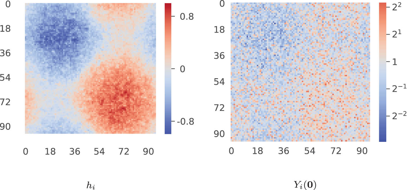
Heatmap of the node homophily feature
6.3 Variance reduction of
τ
ˆ
In this section, we demonstrate the significant variance reduction of the HT estimator under RGCR compared with the standard GCR scheme.
To make the benefits of randomization concrete, for each RGCR design, we study the variance of HT GATE estimators when mixing
The benefit of analyzing mixtures of
In our simulations, we contrast mixtures of
Figure 3 shows the variance of the HT GATE estimator under each unweighted random clustering strategy with independent cluster-level assignment. Within each scheme, we observe enormous variance reduction from randomized clustering in both the synthetic small-world network and the Facebook friendship network. With
![Figure 3
The distribution of
V ar
[
τ
ˆ
]
{\bf{V\; ar}}{[}\hat{\tau }]
when mixing
K
K
random clusterings from the unweighted randomized 3-net and 1-hop-max algorithms in the heavy-tailed Small World network (left) and the FB-Stanford network (right). The number of nodes in each network is marked by a dashed line. We plot the median (solid line) as well as the 2.5 and 97.5% quantiles (shaded area) of the variance distribution from our simulations. For both algorithms and both networks, we observe enormous variance reduction from cluster mixing. Similar trends are also seen in the weighted clustering methods (not shown).](/document/doi/10.1515/jci-2022-0014/asset/graphic/j_jci-2022-0014_fig_003.jpg)
The distribution of
6.4 Exposure probabilities
In Section 6.3, we approximate the RGCR scheme under the random cluster distribution
We first validate the accuracy in this Monte Carlo procedure and then also examine the estimated probabilities, comparing them with the theory developed in Section 4. Again all simulations are conducted under the scenario where we assign each cluster into the treatment group with probability
6.4.1 Accuracy in exposure probabilities estimation
We demonstrate the accuracy of our Monte Carlo procedure for a
of each node
When
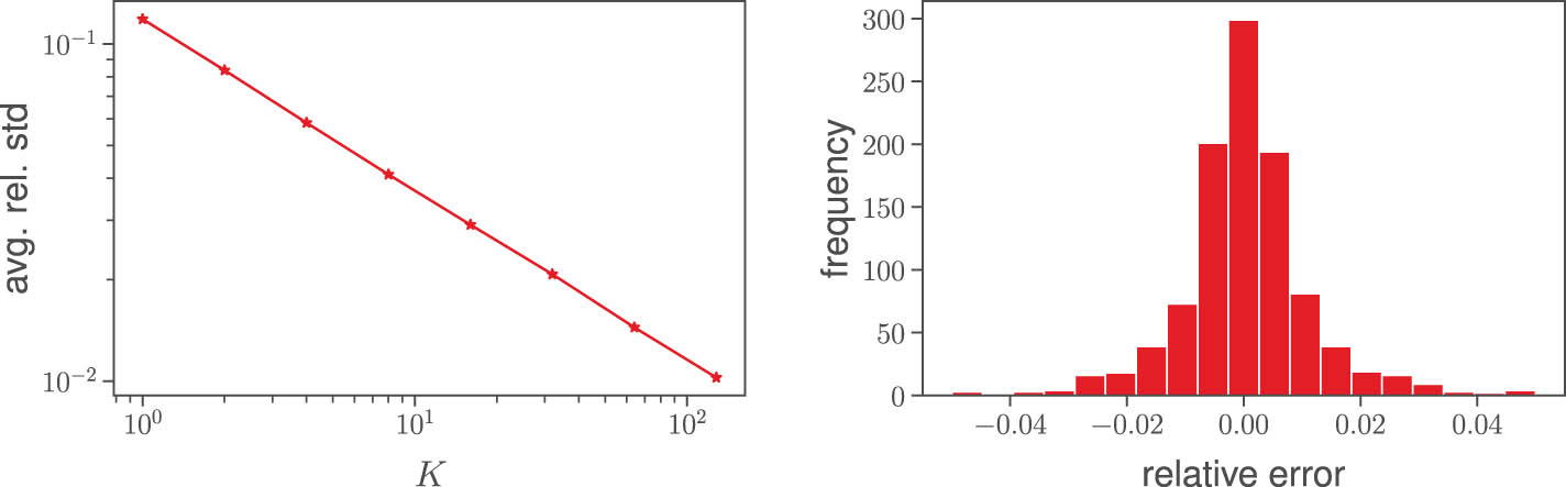
Left: Average relative standard deviation of the exposure probability estimator with
Besides the relative standard deviation, we also examine the distribution of the relative error of a set of estimated exposure probabilities from
where we use the average exposure probability across the 10 repetitions as the ground truth exposure probability of each node. The histogram of the relative errors at all nodes is shown in Figure 4 (right), where we see the relative errors are bounded within
6.4.2 Visualizing exposure probabilities
Figure 5 furnishes a scatterplot of the estimated exposure probabilities under each randomized clustering strategy with cluster-level independent randomization versus the size of the 2-ball at each node. In the first column, where we see the unweighted randomized 3-net and 1-hop-max schemes, the lower bound provided in Theorem 4.2 is verified (blue dashed line), as well as the slightly stronger lower bound for the unweighted 1-hop-max scheme from Theorem 4.3. These lower bounds fall off with
![Figure 5
Scatterplot of the exposure probability
P
[
E
i
1
∣
P
]
{\mathbb{P}}{[}{E}_{i}^{{\bf{1}}}| {\mathcal{P}}]
versus
∣
B
2
(
i
)
∣
| {B}_{2}\left(i)|
at every node
i
i
in the heavy-tailed Small World network (top two rows) and the FB-Stanford network (bottom two rows), under each random clustering scheme with cluster-level independent randomization. The blue dashed line represents the exposure probability lower bound for unweighted 3-net and 1-hop-max schemes (Theorem 4.2). The blue dotted line represents the slightly improved lower bound for unweighted 1-hop-max (Theorem 4.3). The green dashed line represents the uniform lower bound for the spectral-weighted schemes (Theorem B.4).](/document/doi/10.1515/jci-2022-0014/asset/graphic/j_jci-2022-0014_fig_005.jpg)
Scatterplot of the exposure probability
The second and third columns of Figure 5 are associated with the weighted 3-net and 1-hop-max clustering strategies. In the second column, we consider the spectral weighting developed in Appendix B.3, which obey a uniform lower bound (green dashed line) on the exposure probability independent of
We further compare the exposure probability across different schemes in Figure 6. In the first two columns, we examine how the spectral weighting affects nodes’ exposure probabilities associated the randomized 3-net and 1-hop-max clustering respectively. For 3-net, under both networks, spectral weighting effectively increases the exposure probability of nodes whose probability is small under the unweighted 3-net, at a very small cost of decreasing some large exposure probabilities. In contrast, for 1-hop-max clustering, even though spectral weighting can increase the very small exposure probabilities seen in the unweighted scheme, it also significantly decreases the probability of many other nodes. Comparing 3-net clustering and 1-hop-max as in the last column, we observe that the exposure probabilities under 3-net are mostly higher than under 1-hop-max, though the smallest exposure probability under 1-hop-max is higher due to the improved lower bound theory in Theorem 4.3.
![Figure 6
Scatterplot of the exposure probability
P
[
E
i
1
∣
P
]
{\mathbb{P}}{[}{E}_{i}^{{\bf{1}}}| {\mathcal{P}}]
of each node in the Small World network (first row) and FB-Stanford network (second row), with different random clustering strategies. The blue dashed line marks the scenario when the exposure probability under two schemes are same. In the first column, we compare the exposure probability at each node with uniform- (i.e., unweighted) and spectral-weighted random 3-net clustering, and similar comparison for 1-hop-max clustering is given in the second column. In the last column, we compare the exposure probabilities with unweighted 3-net and 1-hop-max clusterings.](/document/doi/10.1515/jci-2022-0014/asset/graphic/j_jci-2022-0014_fig_006.jpg)
Scatterplot of the exposure probability
6.5 HT estimator variance
We now examine the variance of
The variances are obtained from equations (4) to (6), the exact ground-truth variance (available in simulations). In addition to the exposure probability of each node
The results are shown in Figure 7, where we make four observations. First, for both networks and every random clustering and weighting scheme, complete randomization usually yields lower variance than independent randomization. Such variance reduction can be explained by the negative correlation introduced in the cluster-level assignment process, leading to larger values of
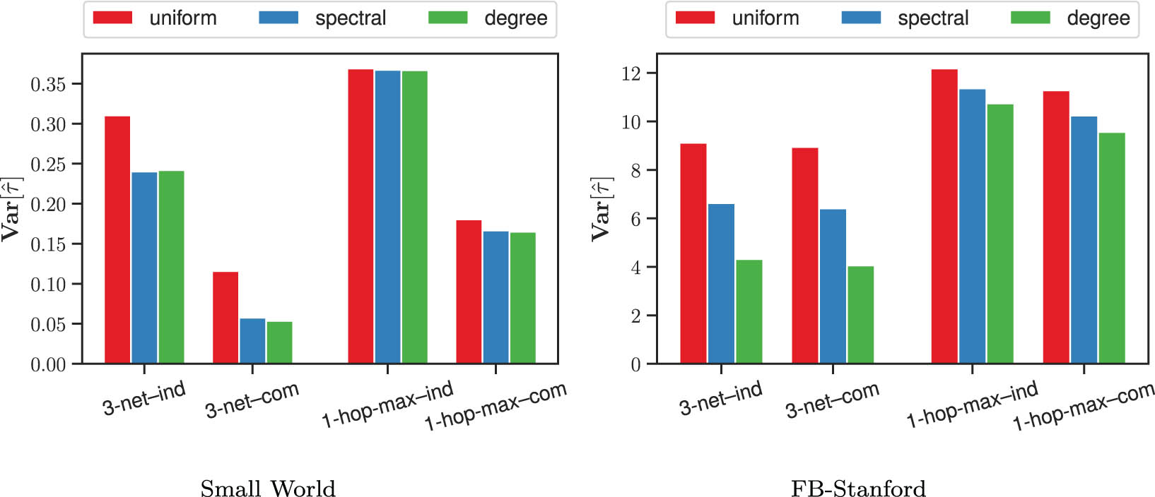
Variance of the HT GATE estimator under the RGCR scheme with various random clustering strategies. The suffix of each clustering method distinguishes independent (- -ind) or complete (- -com) randomization at the cluster level. The variance of these HT estimators under GCR, not shown, are all dramatically higher (comparable to results in Figure 3).
Second, in both networks and with both the 3-net and 1-hop-max random clustering strategy, the variance with the spectral-weighted scheme is lower than that of the unweighted version. Such reduction can be explained by the increase in the lowest exposure probabilities (see the first two columns of Figure 6). This variance reduction is less significant for 1-hop-max clustering, which is consistent with how the spectral-weighted scheme also decreases the exposure probabilities of most nodes (second column of Figure 6).
Third, we observe that degree weighting usually gives lower variance than the spectral-weighted scheme. According to the discussion begun in Appendix B.3, spectral weighting achieves a uniform lower bound on the exposure probability of every node, but this lower bound is less tight for nodes with smaller
We conclude that for HT estimators, RGCR, with randomized 3-net and 1-hop-max are generally comparable. Between the two, randomized 3-net usually yields a modestly lower variance. According to Lemma 4.1, 1-hop-max has a local dependency property, and thus, the cross-node terms in the variance formulae (equations (4)–(6)) decay significantly in the distance between node pairs (and become zero when the distance is greater than 4). In contrast, randomized 3-net has no local dependency guarantee, and consequently, we do not have a nontrivial theoretical upper bound on the variance. However, in our simulations, the cross-node terms are also small, making the variance of the HT estimator under randomized 3-net even lower than using 1-hop-max.
In summary, for the HT GATE estimator for the response model and networks, we study:
complete randomization yields lower variance than independent randomization,
randomized 3-net clustering yields lower variance than 1-hop-max,
spectral- and degree-weighting schemes yields lower variance than unweighted schemes.
6.6 Hájek estimator bias and variance
Unlike the HT estimator, the Hájek estimator does not have close-form formulae to compute the bias, variance, or MSE, and thus, we estimate these quantities via simulation. We therefore briefly describe how we evaluate performance via simulation. For GCR, since the estimation performance is associated with the specific clustering is use, we use the median bias, variance, and MSE across 1,000 randomly generated clusterings. Specifically for each clustering, we simulate the experimental procedure (assignment, outcome generation, and GATE estimation) and compute the sample bias, variance, and MSE and use as the proxy of the corresponding measure of the GCR scheme. For RGCR, we simulate the experimental procedure (random clustering generation, assignment, outcome generation, and GATE estimation)
Figure 8 presents the bias, variance, and MSE of the Hájek estimator under GCR and RGCR, focusing on independent randomization. We make two main observations. First, the bias of the Hájek estimator under RGCR has been significantly reduced, compared with GCR. Recall that in our response model (Section 6.2), the ground-truth GATE is
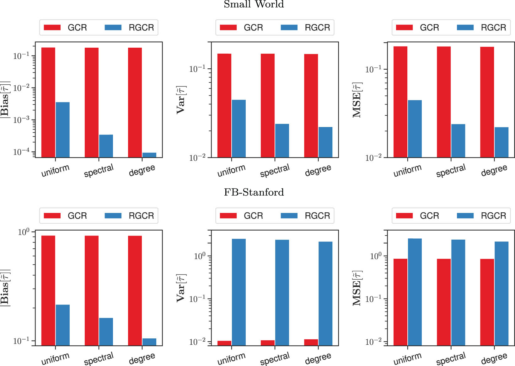
Bias, variance, and MSE of the Hájek GATE estimator under GCR and RGCR with 3-net clustering and independent randomization in the Small World (first row) and FB-Stanford (second row) networks.
One can intuitively interpret this bias reduction as follows. Under GCR, for nodes with exponentially small exposure probability (in the FB-Stanford network, it can be lower than
In contrast, for RGCR, the exposed nodes are not so strictly high exposure probabilities. For example, if a large degree node is at the center of a cluster in a randomly generated clustering, even though it has large conditional exposure probability under this clustering and thus being likely to be network exposure to treatment or control, its unconditional exposure probability can still be small. As a result, it is weighted more heavily in the weighted average procedure of Hájek estimation, making the estimator value shift toward the response of large degree nodes and thus less biased than that under GCR.
Alongside this understanding of Hájek bias, it is also expected to observe an increase in variance from RGCR, vs GCR, under Hájek estimation. In Figure 8, we see variance reduction from RGCR in the Small World network but an increased variance in the FB-Stanford network. Under GCR, since the estimator value is dominated by the response of low degree nodes, in our response model, the response of low-degree nodes have a much narrower range than the whole population, resulting in low variance (but overwhelming bias, we repeat).
Finally, we also compare the bias and MSE of the RGCR scheme with different random clustering strategies, which we also include complete randomization, and the results are given in Figure 9. In general, the benefits of complete randomization (over independent randomization) that we see for the HT estimator do not appear to carry over to Hájek estimation.
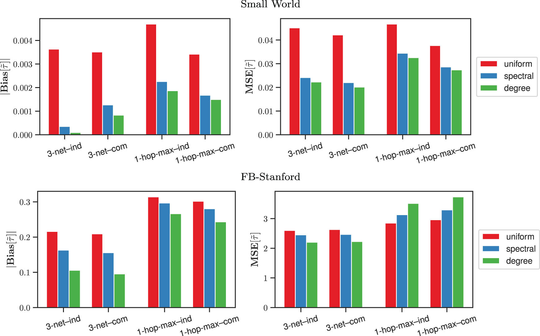
Bias and MSE of Hájek GATE estimator under RGCR with various clustering algorithms with both independent and complete randomization.
In summary, comparing with the GCR scheme, the Hájek estimator under the RGCR scheme has significantly lower bias but may have larger variance. Examining the MSE that trades off bias and variance, we see a lower MSE in the Small World network from RGCR (vs GCR), while we see a higher MSE in the FB-Stanford network under RGCR (vs GCR).
6.7 Variance, bias, and network size
Here, we examine how the bias, variance, and MSE change as a function of network size. Recall that the heavy-tailed small-world network we use throughout our earlier simulations is based on a periodic two-dimensional lattice of side length 96 (thus,
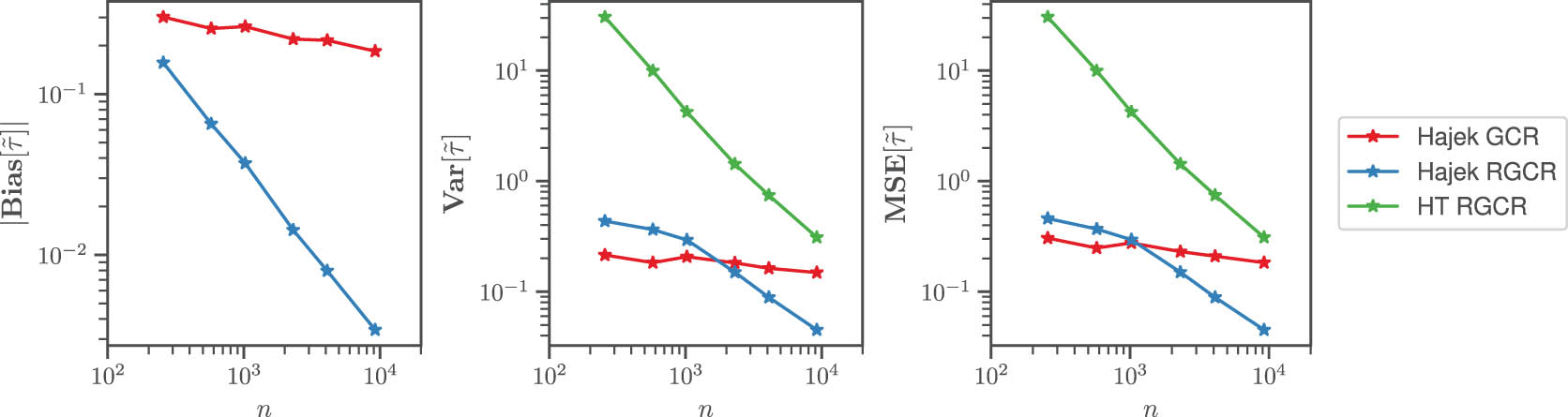
Bias (absolute value), variance, and MSE of the Hájek and HT GATE estimator under GCR and RGCR with unweighted 3-net clustering in a sequence of increasingly sized heavy-tailed small-world networks.
From the first plot in Figure 10, we observe that the Hájek estimator under the RGCR scheme has consistently less bias than under the GCR scheme, across the range of network sizes we study. Moreover, the bias decays with the network size at a much higher rate for RGCR than for GCR. Recall that the HT estimator is unbiased (under both GCR and RGCR).
From the second plot, we observe that the variance of the Hájek estimator under RGCR also decays with higher rate than under GCR. We can explain the slow decay of the variance under GCR by observing that as the number of nodes
Combining both bias and variance, we observe that the MSE of all three methods decays with the network size, while the decay rate is notably faster for the estimators based on the RGCR scheme. In summary, with a large interference network, the Hájek estimator with RGCR is preferred.
7 Conclusion
We developed RGCR as a scheme for the design and analysis of randomized experiments in the presence of interference. This scheme is an improvement on the graph clustering randomization (GCR) scheme in that it is based on a distribution of random clusterings instead of a single fixed clustering, with favorable consequences for the bias and variance of standard estimators. Compared to GCR, the RGCR scheme with proper random clustering generators enjoys significantly reduced variance for both the Horvitz–Thompson and the Hájek estimator of the GATE, and also supports complete randomization. We also discuss how the network drift pattern in node’s responses, as is observed in real-world settings, plays an important role in the variance of GATE estimation, and propose a new response model exhibiting homophily in the form of network drift in responses, facilitating a more careful analysis of realistic estimator performance.
Acknowledgements
We thank Guillaume Basse, Alex Chin, Dean Eckles, and Aaron Sidford for valuable discussions, as well as participants at the Conference on Digital Experimentation (CODE) and at the MIT Initiative on the Digital Economy Seminar.
-
Funding information: This work was supported in part by NSF grant IIS-1657104.
-
Author contributions: All authors have accepted responsibility for the entire content of this manuscript and approved its submission.
-
Conflict of interest: The authors state no conflict of interest.
-
Data availability statement: Replication code available at https://github.com/hyin-stanford/RGCR-code.
Appendix A Empirical study of social network growth rates
As described in Section 1, the theoretical analyses in this work are developed under either a bound on the maximum degree
We use the Facebook100 datasets [67,70,71], a collection of complete Facebook friendship networks at 100 American institutions collected and released in September 2005. The networks are quite diverse, most basically varying in size from 762 to
Network statistics of 25 randomly selected networks from the Facebook-100 collection, listing the number of nodes
| University |
|
|
|
|
|
|
|
|
|||||
|---|---|---|---|---|---|---|---|---|---|---|---|---|---|
|
|
|
|
|
|
|
|
|||||||
| Caltech36 | 762 | 16,651 | 6 | 43.70 | 248 | 102 | 0.0587 | 0.6448 | 0.9618 | 0.9986 | 0.3268 | 0.9357 | 0.9987 |
| Swarthmore42 | 1,657 | 61,049 | 6 | 73.69 | 577 | 149 | 0.0451 | 0.6594 | 0.9790 | 0.9991 | 0.3488 | 0.9523 | 0.9994 |
| Trinity100 | 2,613 | 111,996 | 6 | 85.72 | 404 | 148 | 0.0332 | 0.5735 | 0.9684 | 0.9980 | 0.1550 | 0.9529 | 0.9981 |
| Wellesley22 | 2,970 | 94,899 | 8 | 63.91 | 746 | 160 | 0.0219 | 0.4781 | 0.9221 | 0.9938 | 0.2515 | 0.9232 | 0.9963 |
| Pepperdine86 | 3,440 | 152,003 | 9 | 88.37 | 674 | 301 | 0.0260 | 0.5400 | 0.9420 | 0.9936 | 0.1962 | 0.9340 | 0.9968 |
| Mich67 | 3,745 | 8,1901 | 7 | 43.74 | 419 | 157 | 0.0119 | 0.2945 | 0.8644 | 0.9906 | 0.1121 | 0.8179 | 0.9939 |
| Rice31 | 4,083 | 184,826 | 6 | 90.53 | 581 | 256 | 0.0224 | 0.5434 | 0.9675 | 0.9994 | 0.1425 | 0.9224 | 0.9995 |
| Wake73 | 5,366 | 279,186 | 9 | 104.06 | 1341 | 671 | 0.0196 | 0.5141 | 0.9561 | 0.9973 | 0.2501 | 0.9702 | 0.9983 |
| UChicago30 | 6,561 | 208,088 | 10 | 63.43 | 1624 | 813 | 0.0098 | 0.3375 | 0.8661 | 0.9832 | 0.2477 | 0.9218 | 0.9938 |
| UC64 | 6,810 | 155,320 | 8 | 45.62 | 660 | 282 | 0.0068 | 0.2103 | 0.7921 | 0.9777 | 0.0971 | 0.8026 | 0.9872 |
| WashU32 | 7,730 | 367,526 | 8 | 95.09 | 1794 | 898 | 0.0124 | 0.4244 | 0.9328 | 0.9957 | 0.2322 | 0.9578 | 0.9988 |
| Yale4 | 8,561 | 405,440 | 9 | 94.72 | 2517 | 1259 | 0.0112 | 0.4132 | 0.9082 | 0.9909 | 0.2941 | 0.9429 | 0.9961 |
| Georgetown15 | 9,388 | 425,619 | 11 | 90.67 | 1235 | 618 | 0.0098 | 0.3546 | 0.8946 | 0.9867 | 0.1317 | 0.8838 | 0.9923 |
| Northwestern25 | 10,537 | 488,318 | 9 | 92.69 | 2105 | 1053 | 0.0089 | 0.3624 | 0.9126 | 0.9936 | 0.1999 | 0.9503 | 0.9974 |
| Stanford3 | 11,586 | 568,309 | 9 | 98.10 | 1172 | 587 | 0.0086 | 0.3375 | 0.8529 | 0.9841 | 0.1012 | 0.8443 | 0.9906 |
| USF51 | 13,367 | 321,209 | 8 | 48.06 | 897 | 319 | 0.0037 | 0.1433 | 0.7428 | 0.9785 | 0.0672 | 0.7441 | 0.9915 |
| Northeastern19 | 13,868 | 381,919 | 9 | 55.08 | 968 | 393 | 0.0040 | 0.1721 | 0.8036 | 0.9850 | 0.0699 | 0.8017 | 0.9930 |
| UCSD34 | 14,936 | 443,215 | 9 | 59.35 | 2165 | 1083 | 0.0040 | 0.1877 | 0.8158 | 0.9868 | 0.1450 | 0.9129 | 0.9970 |
| UMass92 | 16,502 | 519,376 | 8 | 62.95 | 3684 | 1843 | 0.0039 | 0.2068 | 0.8621 | 0.9939 | 0.2233 | 0.9575 | 0.9994 |
| UConn91 | 17,206 | 604,867 | 8 | 70.31 | 1709 | 855 | 0.0041 | 0.2082 | 0.8754 | 0.9946 | 0.0994 | 0.9167 | 0.9980 |
| Auburn71 | 18,448 | 973,918 | 7 | 105.59 | 5160 | 2581 | 0.0058 | 0.3672 | 0.9528 | 0.9989 | 0.2798 | 0.9795 | 0.9998 |
| Maryland58 | 20,829 | 744,832 | 7 | 71.52 | 3784 | 1893 | 0.0035 | 0.2031 | 0.8631 | 0.9937 | 0.1817 | 0.9474 | 0.9989 |
| Wisconsin87 | 23,831 | 835,946 | 9 | 70.16 | 3484 | 1620 | 0.0030 | 0.1888 | 0.8607 | 0.9929 | 0.1462 | 0.9361 | 0.9985 |
| Indiana69 | 29,732 | 1,305,757 | 8 | 87.84 | 1358 | 479 | 0.0030 | 0.1794 | 0.8624 | 0.9941 | 0.0457 | 0.8102 | 0.9960 |
| MSU24 | 32,361 | 1,118,767 | 8 | 69.14 | 5267 | 2634 | 0.0022 | 0.1413 | 0.8222 | 0.9913 | 0.1628 | 0.9478 | 0.9989 |
The average growth geometry of the full population of 100 networks in the FB100 collection is illustrated in Figure A1. The more fine-grained growth of the Small World and FB-Stanford networks are illustrated in Figure A2.
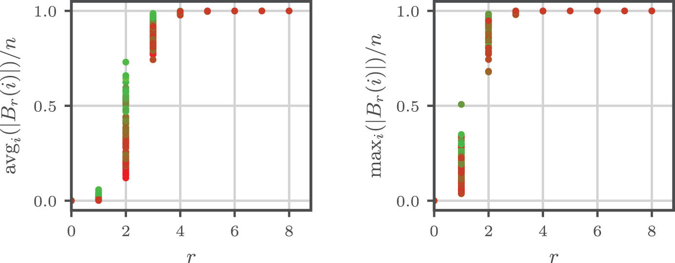
Mean and max ball size at each radius
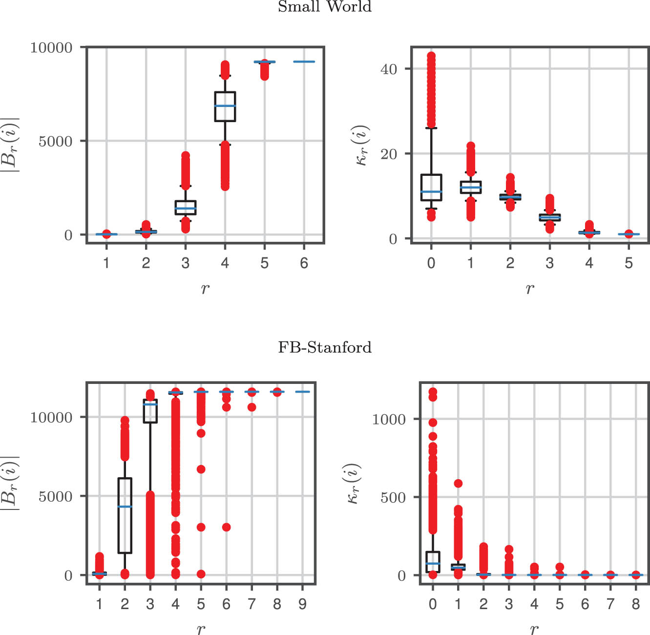
The ball sizes
We here give a concise summary of specific observations from Table A1 and these figures. First, per Table A1, diameter appears to be independent of network size. This is not surprising, as diameter is a fragile metric known to be sensitive to whiskers in the network. Second, the maximum degree, restricted growth coefficient, and network size all appear to be positively correlated. Third, an observation that impacts how we interpret our theoretical results, the restrictive growth coefficients
Looking closer at the results across netowrks in both Table A1 and Figure A1, regarding the average ball-size at each radius
B Weighted algorithms
B.1 Algorithms
Recall that, in the 1-hop-max clustering algorithm (Algorithm 2), we first independently generate a random number from the uniform distribution and construct a clustering based on these generated random numbers: nodes with higher numbers dominate their neighbors and are more likely to be in the center of a cluster. Since the numbers are generated from a uniform distribution, the probability that a given node generates a larger number than any other is always 1/2, making higher-degree nodes less likely to dominate all their neighbors.
| Algorithm 3: Weighted 1-hop-max clustering | |
|---|---|
|
Input: Graph
|
|
|
Output: Graph clustering
|
|
| 1 |
for
|
| 2 |
|
| 3 |
for
|
| 4 |
|
| 5 |
return
|
Our proposed fix to this problem is to change the first step of the algorithm, generating numbers
To understand the intuition behind the weighted scheme, we first note the following basic and well-known properties of the beta distribution, proven for completeness in Appendix C.
Theorem B.1
For independent random variables
According to part (a) of Theorem B.1, a node with a larger weight is more likely to generate a larger number. Thus, by adopting larger weights at high degree nodes, we can make the large degree nodes more likely to dominate their neighbors, correcting their disadvantage in the unweighted scheme.
| Algorithm 4: Weighted 3-net clustering | |
|
Input: Graph
|
|
|
Output: Graph clustering
|
|
| 1 |
for
|
| 2 |
|
| 3 |
|
| 4 |
|
| 5 |
for
|
|
|
|
| 10 |
for
|
| 11 |
|
| 12 |
return
|
This idea of node weighting can also be applied to 3-net clustering. In the unweighted version, we first generate a uniform random ordering of all nodes, which is used to form a seed set and partition the network. In a uniform random ordering where each node has an equal probability of ranking first, large degree nodes are at disadvantage of being selected into the seed set and being the center of a cluster and thus less likely to be network exposed. To compensate for this disadvantage, we can generate a nonuniform random ordering where large degree nodes are more likely to rank high. A nonuniform random ordering can be generated by a combination of Beta-distributed samples and sorting. Specifically, if each node
We note two connections between the weighted 3-net and 1-hop-max clustering algorithms and their original unweighted versions. First, the weighted version can be considered an extension of the unweighted algorithms: when all nodes have the same weight, the weighted 3-net and 1-hop-max algorithm are equivalent to the original algorithm. Second, for either 3-net or 1-hop-max clustering, the distribution of the random clustering returned from the unweighted and weighted algorithms have the same support, i.e., for clusterings that has nonzero probability of being generated from the unweighted version, the probability of being generated from the weighted version is also nonzero, and vice versa. While the support of possible clusterings is the same, certain clusterings are more or less likely to be generated in the weighted versions than the unweighted versions. Consequently, conditioning on the generated clustering and using it in a GCR scheme, there is no difference between which version is used to generate the clustering. However, in RGCR, which is based on a distribution of clusterings, the weighted version might have superior properties due to its node-level adjustments.
B.2 Properties with arbitrary node weights
In this section, we discuss properties of the weighted 3-net and 1-hop-max algorithms with an arbitrary set of node weights. The result motivates our discussion on good choices of node weights in section that follows.
First, we have the following lower bound on exposure probabilities at each node. Similar to Theorem 4.2, the result is based on analyzing the probability that a node is ranked first in its 2-hop-neighborhood. The proof is given in Appendix C.
Theorem B.2
With the weighted 3-net or 1-hop-max random clustering algorithm, using either independent or complete randomization at the cluster level, the full-neighborhood exposure probabilities for any node i satisfy
When all nodes have equal weights, then the weighted 3-net and 1-hop-max algorithm degenerates to the original version, making Theorem B.2 a generalization of Theorem 4.2.
Computing the exposure probability of each node might now be challenging, but we again show that Monte Carlo estimation, as in equation (10), can efficiently achieve low relative error.
Theorem B.3
By using either weighted 3-net or weighted 1-hop-max random clustering algorithm, and with K Monte-Carlo trials, for any node i, the relative error of the Monte-Carlo estimator is upper bounded in MSE as follows:
As stated earlier, stratified sampling can also be adapted for the weighted clustering methods. Similar to the procedure in Section 4.2.2, we generate
Again this stratified method is preferred over Monte Carlo estimation with independent samples since it guarantees positivity in the estimated exposure probabilities and reduces variance in the probability estimation.
B.3 Choice of node weights
With the node-level flexibility in the weighted 3-net and 1-hop-max clustering, a natural subsequent question is to find a good choice of node weights. In this section, we discuss two heuristics that lead to different sets of node weights. The first heuristic suggests node weights based on the eigenvector of an eigenvalue problem associated with the network’s squared adjacency matrix. The second heuristic suggests uniform weights, i.e., the unweighted versions of the algorithms.
B.3.1 Maximizing the minimal exposure probability lower bound
As is discussed in the previous sections, high-degree nodes are less likely than low-degree nodes to be network exposed using the unweighted 3-net or 1-hop-max clustering. To correct this disadvantage, it might be ideal if all nodes have the same exposure probability, or at least the same lower bound.
Given a graph
all the elements
By using these spectral weights in the weighted 3-net or 1-hop-max scheme, we show that as a corollary of Theorem B.2 and equation (A1) (the proof logic is identical), all nodes now have the same exposure probability lower bound.
Theorem B.4
With the spectral-weighted 3-net or 1-hop-max random clustering algorithm, using either independent or complete randomization at the cluster level, the full-neighborhood exposure probabilities for any node i satisfy
a uniform lower bound on the full neighborhood exposure probability of all nodes.
We then have the following corollary (of Theorem 4.7) upper bound on the variance of HT GATE estimators using RGCR with spectral-weighted 1-hop-max random clustering.
Theorem B.5
Using RCGR with spectral-weighted 1-hop-max clustering, if every node’s response is within
for both independent and complete cluster-level randomization.
Proof
We first note that, with an identical proof, one can verify that Theorem 4.6 also hold with the weighed 1-hop-max clustering with any weights
where the first inequality is due to the exposure probability lower bound in Theorem B.4.□
As a final corollary, we have the following upper bound on the variance of the HT GATE estimator, by a proof identical to that of Theorem 4.8.
Theorem B.6
Using RCGR with spectral-weighted 1-hop-max clustering, if every node’s response is within
for both independent and complete cluster-level randomization.
Of note, according to the Perron-Frobenius theorem, we also have
As a result, this variance upper bound using spectral-weighted 1-hop-max clustering can be used to furnish the variance upper bound for the unweighted 1-hop-max clustering (Theorem 4.8) as well. These final inequalities are not necessarily strict improvements – they become equalities for a regular graph – but in practical settings, they can lead to sizable improvements over unweighted clustering methods.
Having the same exposure probabilities at each node is ideal, whereas we note that our spectral weights do not exactly achieve that. They merely maximize a uniform lower bound, the lower bound given in Theorem B.2. The tightness of this lower bound might not be equal at each node, since it only captures the scenario when the node is at the interior of a cluster. If a node is not in the interior and thus adjacent to multiple clusters, then a lower-degree node is likely to be adjacent to fewer clusters and thus still has higher exposure probability. Therefore, in reality, one might use a weight where high-degree nodes are even more aggressively favored than under spectral weighting. In Section 6, besides uniform weight and spectral weight, we also consider weighting each node by their degree directly. Simulation results show that this aggressive degree weight strategy usually yields lower variance than both uniform weights and spectral weights.
B.3.2 Minimizing a variance proxy
The aforementioned heuristic is intended to reduce the estimator variance, but a more direct approach would be to find the optimal weights that minimize the actual estimator variance.
That said, optimizing the variance, as formulated in equations (4) to (6), is challenging because (i) it consists of cross-terms associated with the joint exposure probability of node pairs that are hard to analyze, and (ii) the nodes’ response is unknown before the experiment, but can play a significant role in determining the variance. One compromise is to use a proxy objective function that resembles the variance formula. We consider the following function
which overlooks the cross-terms and assumes a uniform response from all nodes.
Note that this proxy function is also intractable since one cannot efficiently compute the exposure probability of each node given the weights. However, one can obtain an upper bound of
and attempt to minimize this variance surrogate. We have the following result.
Theorem B.7
The minimum of
for any
The first heuristic increased the exposure probability of high degree nodes, but came at the cost of decreasing the exposure probabilities of low degree nodes. Thus, it is not certain whether this heuristic would actually reduces variance. It is therefore interesting that under this second heuristic, if trusting
The construction of the surrogate variance,
C Proofs
C.1 Proof of Theorem 4.1
Proof
In the first step of the algorithm (line 1–2), every node independently generates a random number which can be executed in parallel. Therefore, the depth is
C.2 Proof of Theorem 4.2
Proof
We first show that the probability that node
To this end, we consider a sufficient condition of this event, for the 3-net clustering and 1-hop-max clustering separately. With 3-net clustering, in the first step when we generate a random ordering of all nodes, if node
Now we derive the results in the theorem. Conditioning on the event that node
With the same reasoning, it can be easily verified that
C.3 Proof of Theorem 4.3
Proof
By symmetry, we only need to consider treatment (control is analogous). Suppose node
where we use the fact that the probability of node
C.4 Proof of Theorem 4.4
Proof
Here, we provide a proof for the specific case
We present a polynomial-time reduction to network exposure probability computation from the minimum maximal distance-3 independent set (MD3IS) problem, which is known to be NP-complete [72]. This problem is as follows.
Minimum Maximal Distance-3 Independent Set problem (decision version): Given a graph
for any pair of nodes
For any instance of the MD3IS problem with input
Before connecting this exposure probability computation problem with the original MD3IS instance, we first present several properties of the maximal distance-3 independent sets of
Lemma C.1
For any node subset in the original graph
Lemma C.2
Any maximal distance-3 independent set of
Lemma C.2 illustrates the two types of maximal distance-3 independent set of
Lemma C.3
For a random sample of 3-net clustering c on
with probability
with probability
Now we have the following key result connecting the exposure probability value to the MD3IS problem.
Lemma C.4
The exposure probability value of node
If there exists a maximal distance-3 independent set of size
If every maximal distance-3 independent set is of size
Combining the aforementioned results, we show that exact computation of the exposure probability solves the MD3IS instance. Suppose there is a polynomial algorithm such that, for any graph
Now according to scenario (2) in Lemma C.4, the MD3IS instance must have a maximal distance-3 independent set of size
and thus, the MD3IS instance cannot have a maximal distance-3 independent set of size
Given this reduction, we must show that the reduction from the MD3IS is polynomial. The size of the MD3IS problem is
and the log value of required precision
Before presenting the proof of Lemma C.1, we first give an auxiliary result.
Lemma C.5
For any distinct nodes
Proof
“
“
Proof (Lemma C.1)
Note that a corollary of Lemma C.5 is the following:
We first show the sufficiency in Lemma C.1. If
Next we show the necessity in Lemma C.1. If
Proof (Lemma C.2)
Suppose
Proof (Lemma C.3)
In 3-net clustering, we use the randomized greedy algorithm to construct a maximal distance-3 independent set as the seed set. With probability
Similarly, with probability
Proof (Lemma C.4)
For the first result, if the MD3IS problem has a maximal distance-3 independent set of size
where the first term comes from the case when a single-node maximal distance-3 independent set is used as seeds.
For the second result, if every maximal distance-3 independent set of size
C.5 Proof of Theorem 4.5
Proof
Unless otherwise stated, all the expectation and variance in this proof are taken conditioned on the random clustering distribution
Let
Consider the Bernoulli random variable
Moreover, note that
and thus,
where the second inequality is due to Theorem 4.2.
Now to prove the inequality in Theorem 4.5, we note that
and thus,
Now note that the expected value of
C.6 Proof of Theorem 4.6
We first present the following result on the joint exposure probability of a pair of nodes.
Lemma C.6
For the 1-hop-max random clustering algorithm, if
independent randomization, we have
complete randomization, we have
Proof
We first show that nodes
Now we prove the results in the lemma. Due to symmetry, it suffices to just prove for the case of
where the last but one equality is due to
We now prove the result for the complete randomization scenario. The proof is almost identical to that of independent randomization, except for the fact that
where the last equality is verified in the proof for independent randomization.□
With this lemma in hand, we now prove Theorem 4.6.
Proof (Theorem 4.6)
According to Lemma C.6, for any pair of nodes
where the second inequality is due to
C.7 Proof of Theorem 4.8
Proof
Analogous to Theorem 4.7, it can be verified that
where the second inequality is due to the mean inequality, and the last inequality is due to the variance upper bound of
C.8 Proof of Theorem 4.10
Proof
With a constant treatment effect
and consequently,
where the second equality is due to the symmetry of network exposure to treatment and control, more specifically, the joint distribution of
Since
C.9 Proof of Theorem 5.1
Proof
Note that in any oracle
For any node pair
a quantity in
C.9.1 Variance under independent randomization
We start with computing the joint exposure probabilities
By combining with equation (A7), we have
and
Now we compute the variance of the mean outcome HT estimators given these probabilities. Note that the variance, as given in equation (4), is equivalent to
due to the fact that
where the third equality is due to the average of
Analogously, it can be shown that
Consequently,
C.9.2 Variance under complete randomization
We also first compute the joint exposure probabilities
and thus,
Similarly, one can show that
With these exposure probabilities, we have
Analogously, it can be shown that
Consequently,
C.9.3 Variance with increasing number of clusters
In the end, we show the variance when the number of clusters
Under the complete randomization scheme, we have
C.10 Proof of Theorem B.1
Proof
For result (a), Since the PDF of
For result (b), we have
which is the CDF of the
C.11 Proof of Theorem B.2
We first prove the following useful lemma.
Lemma C.7
If every node generates
Proof
According to the second result in Theorem B.1, the distribution of
Proof (Theorem B.2)
Analogous to the proof of Theorem 4.2, one only need to show that the probability of node
For 1-hop-max clustering, similarly a sufficient condition for node
For 3-net clustering, again we consider the scenario when node
C.12 Proof of Theorem B.3
The proof is almost the same as that of Theorem 4.5, except that in equation (A5), we apply the lower bound result of Theorem B.2.
C.13 Proof of Theorem B.7
Proof
Note that
where the inequality applies the AM–GM inequality, which holds as equality if all nodes have the same weight.□
References
[1] Hudgens MG, Halloran ME. Toward causal inference with interference. J Amer Stat Assoc. 2008;103(482):832–42. 10.1198/016214508000000292Search in Google Scholar PubMed PubMed Central
[2] Fienberg SE. A brief history of statistical models for network analysis and open challenges. J Comput Graph Stat. 2012;21(4):825–39. 10.1080/10618600.2012.738106Search in Google Scholar
[3] Aronow PM, Samii C. Estimating average causal effects under general interference, with application to a social network experiment. Ann Appl Stat. 2017;11(4):1912–47. 10.1214/16-AOAS1005Search in Google Scholar
[4] Sävje F, Aronow P, Hudgens M. Average treatment effects in the presence of unknown interference. Ann Stat. 2021;49(2):673. 10.1214/20-AOS1973Search in Google Scholar
[5] Chin A. Central limit theorems via stein’s method for randomized experiments under interference. 2018. arXiv: http://arXiv.org/abs/arXiv:1804.03105. Search in Google Scholar
[6] Jagadeesan R, Pillai NS, Volfovsky A. Designs for estimating the treatment effect in networks with interference. Ann Stat. 2020;48(2):679–712. 10.1214/18-AOS1807Search in Google Scholar
[7] Eckles D, Karrer B, Ugander J. Design and analysis of experiments in networks: reducing bias from interference. J Causal Infer. 2017;5(1):20150021. 10.1515/jci-2015-0021Search in Google Scholar
[8] Saint-Jacques G, Varshney M, Simpson J, Xu Y. Using ego-clusters to measure network effects at linkedin. 2019. arXiv: http://arXiv.org/abs/arXiv:1903.08755. Search in Google Scholar
[9] Chin A. Regression adjustments for estimating the global treatment effect in experiments with interference. J Causal Infer. 2019;7(2). 10.1515/jci-2018-0026Search in Google Scholar
[10] Saveski M, Pouget-Abadie J, Saint-Jacques G, Duan W, Ghosh S, Xu Y, et al. Detecting network effects: Randomizing over randomized experiments. In: Proceedings of the 23rd ACM SIGKDD International Conference on Knowledge Discovery and Data Mining; 2017. p. 1027–35. 10.1145/3097983.3098192Search in Google Scholar
[11] Pouget-Abadie J, Mirrokni V, Parkes DC, Airoldi EM. Optimizing cluster-based randomized experiments under monotonicity. In: Proceedings of the 24th ACM SIGKDD International Conference on Knowledge Discovery and Data Mining. 2018. p. 2090–9. 10.1145/3219819.3220067Search in Google Scholar
[12] Pouget-Abadie J, Saint-Jacques G, Saveski M, Duan W, Ghosh S, Xu Y, et al. Testing for arbitrary interference on experimentation platforms. Biometrika. 2019;106(4):929–40. 10.1093/biomet/asz047Search in Google Scholar
[13] Blake T, Coey D. Why marketplace experimentation is harder than it seems: the role of test-control interference. In: Proceedings of the Fifteenth ACM Conference on Economics and Computation; 2014. p. 567–82. 10.1145/2600057.2602837Search in Google Scholar
[14] Fradkin A. A simulation approach to designing digital matching platforms. Boston University Questrom School of Business Research Paper Forthcoming; 2019. https://papers.ssrn.com/sol3/papers.cfm?abstract_id=3320080.10.2139/ssrn.3320080Search in Google Scholar
[15] Ha-Thuc V, Dutta A, Mao R, Wood M, Liu Y. A counterfactual framework for seller-side a/b testing on marketplaces. In: Proceedings of the 43rd International ACM SIGIR Conference on Research and Development in Information Retrieval, New York, NY, USA; 2020. p. 2288–96. 10.1145/3397271.3401434Search in Google Scholar
[16] Holtz D, Aral S. Limiting bias from test-control interference in online marketplace experiments. 2020. arXiv: http://arXiv.org/abs/arXiv:2004.12162. 10.2139/ssrn.3583596Search in Google Scholar
[17] Johari R, Li H, Liskovich I, Weintraub GY. Experimental design in two-sided platforms: an analysis of bias. Management Sci. 2022;68(10):7069–89. 10.1287/mnsc.2021.4247Search in Google Scholar
[18] Ogburn EL, VanderWeele TJ. Causal diagrams for interference. Stat Sci. 2014;29(4):559–78. 10.1214/14-STS501Search in Google Scholar
[19] Ogburn EL, Shpitser I, Lee Y. Causal inference, social networks and chain graphs. J R Stat Soc Ser A (Stat Soc) 2020;183(4):1659–76. 10.1111/rssa.12594Search in Google Scholar PubMed PubMed Central
[20] Cox DR. Planning of Experiments. New York: Wiley; 1958. Search in Google Scholar
[21] Rubin DB. Estimating causal effects of treatments in randomized and nonrandomized studies. J Educat Psychol. 1974;66(5):688. 10.1037/h0037350Search in Google Scholar
[22] Sobel ME. What do randomized studies of housing mobility demonstrate? causal inference in the face of interference. J Amer Stat Assoc. 2006;101(476):1398–407. 10.1198/016214506000000636Search in Google Scholar
[23] Manski CF. Identification of treatment response with social interactions. Econom J. 2013;16(1):S1–23. 10.1111/j.1368-423X.2012.00368.xSearch in Google Scholar
[24] Choi D. Estimation of monotone treatment effects in network experiments. J Amer Stat Assoc. 2017;112(519):1147–55. 10.1080/01621459.2016.1194845Search in Google Scholar
[25] Sussman DL, Airoldi EM. Elements of estimation theory for causal effects in the presence of network interference. 2017. arXiv: http://arXiv.org/abs/arXiv:1702.03578. Search in Google Scholar
[26] Forastiere L, Airoldi EM, Mealli F. Identification and estimation of treatment and interference effects in observational studies on networks. J Amer Stat Assoc. 2021;116(534)901–18. 10.1080/01621459.2020.1768100Search in Google Scholar
[27] Ugander J, Karrer B, Backstrom L, Kleinberg J. Graph cluster randomization: network exposure to multiple universes. In: Proceedings of the 19th ACM SIGKDD International Conference on Knowledge Discovery and Data Mining. ACM; 2013. p. 329–37. 10.1145/2487575.2487695Search in Google Scholar
[28] Horvitz DG, Thompson DJ. A generalization of sampling without replacement from a finite universe. J Amer Stat Assoc. 1952;47(260):663–85. 10.1080/01621459.1952.10483446Search in Google Scholar
[29] VanderWeele TJ. Concerning the consistency assumption in causal inference. Epidemiology. 2009;20(6):880–3. 10.1097/EDE.0b013e3181bd5638Search in Google Scholar PubMed
[30] Yu CL, Airoldi EM, Borgs C, Chayes JT. Estimating the total treatment effect in randomized experiments with unknown network structure. Proc National Acad Sci. 2022;119(44):e2208975119. 10.1073/pnas.2208975119Search in Google Scholar PubMed PubMed Central
[31] Basu D. An essay on the logical foundations of survey sampling, Part I. In: Godambe V, Sprott D, editors. Foundations of statistical inferences, Toronto, Canada: Holt, Rinehart and Winston; 1971. Search in Google Scholar
[32] Kojevnikov D, Marmer V, Song K. Limit theorems for network dependent random variables. J Econom. 2021;222(2):882–908. 10.1016/j.jeconom.2020.05.019Search in Google Scholar
[33] Leung MP. Causal inference under approximate neighborhood interference. Econometrica. 2022;90(1):267–93. 10.3982/ECTA17841Search in Google Scholar
[34] Leskovec J, Horvitz E. Planetary-scale views on a large instant-messaging network. In: Proceedings of the 17th international conference on World Wide Web; 2008. p. 915–24. 10.1145/1367497.1367620Search in Google Scholar
[35] Backstrom L, Boldi P, Rosa M, Ugander J, Vigna S. Four degrees of separation. In: Proceedings of the 4th Annual ACM Web Science Conference; 2012. p. 33–42. 10.1145/2380718.2380723Search in Google Scholar
[36] Ugander J, Karrer B, Backstrom L, Marlow C. The anatomy of the Facebook social graph. 2011. arXiv: http://arXiv.org/abs/arXiv:1111.4503. Search in Google Scholar
[37] Travers J, Milgram S. An experimental study of the small world problem. Sociometry. 1969;32(4):425–43. 10.2307/2786545Search in Google Scholar
[38] Radaelli L, Sapiezynski P, Houssiau F, Shmueli E, de Montjoye Y-A. Quantifying Surveillance in the Networked Age: Node-based Intrusions and Group Privacy. 2018. arXiv: http://arXiv.org/abs/arXiv:1803.09007. Search in Google Scholar
[39] Su J, Sharma A, Goel S. The effect of recommendations on network structure. In: Proceedings of the 25th International Conference on World Wide Web; 2016. p. 1157–67. 10.1145/2872427.2883040Search in Google Scholar
[40] Spielman DA, Teng S-H. Spectral partitioning works: Planar graphs and finite element meshes. In: Proceedings of 37th Conference on Foundations of Computer Science; 1996. p. 96–105. 10.1109/SFCS.1996.548468Search in Google Scholar
[41] Shi J, Malik J. Normalized cuts and image segmentation. IEEE Trans Pattern Anal Machine Intell. 2000;22(8):888–905. 10.1109/34.868688Search in Google Scholar
[42] Lee JR, Gharan SO, Trevisan L. Multiway spectral partitioning and higher-order cheeger inequalities. JACM. 2014;61(6):1–30. 10.1145/2665063Search in Google Scholar
[43] Ugander J, Backstrom L. Balanced label propagation for partitioning massive graphs. In: Proceedings of the Sixth ACM International Conference on Web Search and Data Mining; 2013. p. 507–16. 10.1145/2433396.2433461Search in Google Scholar
[44] Nishimura J, Ugander J. Restreaming graph partitioning: simple versatile algorithms for advanced balancing. In: Proceedings of the 19th ACM SIGKDD International Conference on Knowledge Discovery and Data Mining; 2013. p. 1106–14. 10.1145/2487575.2487696Search in Google Scholar
[45] McPherson M, Smith-Lovin L, Cook JM. Birds of a feather: homophily in social networks. Ann Rev Sociol. 2001;27(1):415–44. 10.1146/annurev.soc.27.1.415Search in Google Scholar
[46] Karger DR, Ruhl M. Finding nearest neighbors in growth-restricted metrics. In: Proceedings of the Thiry-fourth Aannual ACM Smposium on Theory of Computing; 2002. p. 741–50. 10.1145/509907.510013Search in Google Scholar
[47] Leskovec J, Kleinberg J, Faloutsos C. Graph evolution: densification and shrinking diameters. ACM Trans Knowledge Discovery Data (TKDD). 2007;1(1):2–es. 10.1145/1217299.1217301Search in Google Scholar
[48] Linial N, Saks M. Low diameter graph decompositions. Combinatorica. 1993;13(4):441–54. 10.1007/BF01303516Search in Google Scholar
[49] Alon N, Babai L, Itai A. A fast and simple randomized parallel algorithm for the maximal independent set problem. J Algorithms. 1986;7(4):567–83. 10.1016/0196-6774(86)90019-2Search in Google Scholar
[50] Miller GL, Peng R, Chen Xu S. Parallel graph decompositions using random shifts. In: Proceedings of the Twenty-fifth Annual ACM Symposium on Parallelism in Algorithms and Architectures; 2013. p. 196–203. 10.1145/2486159.2486180Search in Google Scholar
[51] Calinescu G, Karloff H, Rabani Y. Approximation algorithms for the 0-extension problem. SIAM J Comput. 2005;34(2):358–72. 10.1137/S0097539701395978Search in Google Scholar
[52] Karzanov AV. Minimum 0-extensions of graph metrics. Europ J Combinatorics. 1998;19(1):71–101. 10.1006/eujc.1997.0154Search in Google Scholar
[53] Dahlhaus E, Johnson DS, Papadimitriou CH, Seymour PD, Yannakakis M. The complexity of multiway cuts. In: Proceedings of the Twenty-fourth Annual ACM Symposium on Theory of Computing; 1992. p. 241–51. 10.1145/129712.129736Search in Google Scholar
[54] Fakcharoenphol J, Rao S, Talwar K. A tight bound on approximating arbitrary metrics by tree metrics. J Comput Syst Sci. 2004;69(3):485–97. 10.1016/j.jcss.2004.04.011Search in Google Scholar
[55] Gupta A, Krauthgamer R, Lee JR. Bounded geometries, fractals, and low-distortion embeddings. In: Proceedings of the 44th Annual IEEE Symposium on Foundations of Computer Science, 2003. IEEE; 2003. p. 534–43. 10.1109/SFCS.2003.1238226Search in Google Scholar
[56] Gleich DF, Seshadhri C. Vertex neighborhoods, low conductance cuts, and good seeds for local community methods. In: Proceedings of the 18th ACM SIGKDD International Conference on Knowledge Discovery and Data Mining; 2012. p. 597–605. 10.1145/2339530.2339628Search in Google Scholar
[57] Yin H, Benson AR, Leskovec J. The local closure coefficient: a new perspective on network clustering. In: Proceedings of the Twelfth ACM International Conference on Web Search and Data Mining; 2019. p. 303–11. 10.1145/3289600.3290991Search in Google Scholar
[58] Blelloch GE, Fineman JT, Shun J. Greedy sequential maximal independent set and matching are parallel on average. In: Proceedings of the Twenty-Fourth Annual ACM Symposium on Parallelism in Algorithms and Architectures. ACM; 2012. p. 308–17. 10.1145/2312005.2312058Search in Google Scholar
[59] Blelloch GE. Programming parallel algorithms. Commun ACM. 1996;39(3):85–97. 10.1145/227234.227246Search in Google Scholar
[60] Trotter HF, Tukey JW. Conditional monte carlo for normal samples. In: Symposium on Monte Carlo Methods. 1956. p. 64. Search in Google Scholar
[61] Swaminathan A, Joachims T. The self-normalized estimator for counterfactual learning. In: Advances in neural information processing systems; 2015. p. 3231–39. Search in Google Scholar
[62] Shalizi CR, Thomas AC. Homophily and contagion are generically confounded in observational social network studies. Sociol Meth Res. 2011;40(2):211–39. 10.1177/0049124111404820Search in Google Scholar PubMed PubMed Central
[63] Kleinberg J. The small-world phenomenon: an algorithmic perspective. In: Proceedings of the Thirty-second Annual ACM Symposium on Theory of Computing; 2000. p. 163–70. 10.1145/335305.335325Search in Google Scholar
[64] Watts DJ, Strogatz SH. Collective dynamics of ‘small-world’ networks. Nature. 1998;393(6684):440. 10.1038/30918Search in Google Scholar PubMed
[65] Milgram S. The small world problem. Psychol Today. 1967;2(1):60–7. 10.1037/e400002009-005Search in Google Scholar
[66] Clauset A, Shalizi CR, Newman MEJ. Power-law distributions in empirical data. SIAM Review. 2009;51(4):661–703. 10.1137/070710111Search in Google Scholar
[67] Traud AL, Mucha PJ, Porter MA. Social structure of facebook networks. Phys A Stat Mech Appl. 2012;391(16):4165–80. 10.1016/j.physa.2011.12.021Search in Google Scholar
[68] Basse GW, Airoldi EM. Model-assisted design of experiments in the presence of network-correlated outcomes. Biometrika. 2018;105(4):849–58. 10.1093/biomet/asy036Search in Google Scholar
[69] VonLuxburg U. A tutorial on spectral clustering. Stat Comput. 2007;17(4):395–416. 10.1007/s11222-007-9033-zSearch in Google Scholar
[70] Traud AL, Kelsic ED, Mucha PJ, Porter MA. Comparing community structure to characteristics in online collegiate social networks. SIAM Review. 2011;53(3):526–43. 10.1137/080734315Search in Google Scholar
[71] Jacobs AZ, Way SF, Ugander J, Clauset A. Assembling thefacebook: Using heterogeneity to understand online social network assembly. In: Proceedings of the ACM Web Science Conference; 2015. p. 1–10. 10.1145/2786451.2786477Search in Google Scholar
[72] Eto H, Guo F, Miyano E. Distance-d independent set problems for bipartite and chordal graphs. J Comb Optim. 2014;27(1):88–99. 10.1007/s10878-012-9594-4Search in Google Scholar
© 2023 the author(s), published by De Gruyter
This work is licensed under the Creative Commons Attribution 4.0 International License.
Articles in the same Issue
- Research Articles
- Adaptive normalization for IPW estimation
- Matched design for marginal causal effect on restricted mean survival time in observational studies
- Robust inference for matching under rolling enrollment
- Attributable fraction and related measures: Conceptual relations in the counterfactual framework
- Causality and independence in perfectly adapted dynamical systems
- Sensitivity analysis for causal decomposition analysis: Assessing robustness toward omitted variable bias
- Instrumental variable regression via kernel maximum moment loss
- Randomization-based, Bayesian inference of causal effects
- On the pitfalls of Gaussian likelihood scoring for causal discovery
- Double machine learning and automated confounder selection: A cautionary tale
- Randomized graph cluster randomization
- Efficient and flexible mediation analysis with time-varying mediators, treatments, and confounders
- Minimally capturing heterogeneous complier effect of endogenous treatment for any outcome variable
- Quantitative probing: Validating causal models with quantitative domain knowledge
- On the dimensional indeterminacy of one-wave factor analysis under causal effects
- Heterogeneous interventional effects with multiple mediators: Semiparametric and nonparametric approaches
- Exploiting neighborhood interference with low-order interactions under unit randomized design
- Robust variance estimation and inference for causal effect estimation
- Bounding the probabilities of benefit and harm through sensitivity parameters and proxies
- Potential outcome and decision theoretic foundations for statistical causality
- 2D score-based estimation of heterogeneous treatment effects
- Identification of in-sample positivity violations using regression trees: The PoRT algorithm
- Model-based regression adjustment with model-free covariates for network interference
- All models are wrong, but which are useful? Comparing parametric and nonparametric estimation of causal effects in finite samples
- Confidence in causal inference under structure uncertainty in linear causal models with equal variances
- Special Issue on Integration of observational studies with randomized trials - Part II
- Personalized decision making – A conceptual introduction
- Precise unbiased estimation in randomized experiments using auxiliary observational data
- Conditional average treatment effect estimation with marginally constrained models
- Testing for treatment effect twice using internal and external controls in clinical trials