Causality and independence in perfectly adapted dynamical systems

2.1 Causal discovery

The main objective of causal discovery is to infer causal relations from experimental and observational data. The most common causal discovery algorithms can be roughly divided into score-based and constraint-based approaches. In this work, we will focus on the latter approach (examples include PC, FCI, and variants thereof, and see [1,2,4,5,7,9,10]), which exploits conditional independences in data to infer causal relations. We will first discuss assumptions for constraint-based causal discovery. We then consider the application of causal discovery algorithms to models with feedback. We proceed with a brief but concrete introduction to a simple causal discovery algorithm. Finally, we discuss how the present work relates to the existing literature.

Learning a graphical structure from conditional independence constraints typically relies on Markov and faithfulness assumptions relating conditional independences to properties of a graph. In particular, a d-separation is a relation between three disjoint sets of vertices in a graph that indicates whether all paths between two sets of vertices are d -blocked by the vertices in a third [3,4]. If every d -separation in a graph implies a conditional independence in the probability distribution, then we say that the distribution satisfies the directed global Markov property (or the d-separation criterion) with respect to that graph [20]. Conversely, if every conditional independence in the probability distribution corresponds to a d -separation in a graph, then we say that the distribution is d-faithful to that graph.^[1] When a probability distribution satisfies the d -separation Markov property with respect to a graph and is also d -faithful to the graph, then this graph is a compact representation of the conditional independences in the probability distribution, and we say that it encodes its independence relations. A lot of work has been done to understand the (combinations of) various assumptions (e.g., linearity, Gaussianity, discreteness, causal sufficiency, acyclicity, no selection bias) under which a graph that encodes all conditional independences and dependences in a probability distribution has a certain causal interpretation [see, e.g., 2,4–10,21,22]. Perhaps the simplest assumption is that the data were generated by a causal directed acyclic graph (DAG) [3,4].^[2] This graphical object represents both the conditional independence structure (the observational probability distribution is assumed to satisfy the directed global Markov property with respect to the graph) and the causal structure (every directed edge that is absent in the DAG corresponds with the absence of a direct causal relation between the two variables, relative to the set of variables in the DAG). For this acyclic setting, sophisticated constraint-based causal discovery algorithms (such as the PC and FCI algorithms [4,5]) have been developed. The key assumption that these algorithms make is that the same DAG expresses both the conditional independences in the observational distribution and the causal relations between the variables.

However, many systems of interest in various scientific disciplines (e.g., biology, econometrics, physics) include feedback mechanisms. Cyclic structural causal models (SCMs) can be used to model causal features and conditional independence relations of systems that contain cyclic causal relationships [23]. For linear SCMs with causal cycles, several causal discovery algorithms have been developed that are based on d -separations [2,6,21,22]. The d -separation criterion is applicable to acyclic settings and to cyclic SCMs with either discrete variables or linear relations between continuous variables, but it is too strong in general [24]. A weaker Markov property, based on the notion of σ -separation, has been derived for graphs that may contain cycles [23–25]. If every σ -separation in a graph implies a conditional independence in the probability distribution then we say that it satisfies the generalized directed global Markov property (or the σ -separation criterion) with respect to that graph [25]. Conversely, if every conditional independence in the probability distribution corresponds to a σ -separation in a graph then we say that it is σ -faithful to that graph. Richardson [26] already proposed a causal discovery algorithm that is sound under the generalized directed Markov property and the d -faithfulness assumption, assuming causal sufficiency. Recently, a causal discovery algorithm was proposed based on the σ -separation criterion and the assumption of σ -faithfulness that is sound and complete [8]. It was also shown that, perhaps surprisingly, the PC and FCI algorithms are still sound and complete in that setting, although their output has to be interpreted differently [10].

For the sake of simplicity, we will limit our attention in this article to one of the simplest causal discovery algorithms, local causal discovery (LCD) [1]. This algorithm is a straightforward and efficient search method to detect a specific causal structure from background knowledge and observational or experimental data. The algorithm looks for triples of variables ( C , X , Y ) for which (a) C is a variable that is not caused by X , and (b) the following (in)dependences hold: C ⊥̸ ⊥ X , X ⊥̸ ⊥ Y , and C ⊥ ⊥ Y ∣ X . Figure 1 shows all acyclic directed mixed graphs (ADMGs)^[3] that correspond to the LCD triple ( C , X , Y ) , assuming d -faithfulness and no selection bias. They all have in common that there is no bidirected edge between X and Y , while there is a directed edge from X to Y . Hence, we can conclude that X causes Y and the two variables are not confounded. The algorithm was proven to be sound in both the σ - and d -separation settings even when cycles may be present [9]. Even though this algorithm is not as sophisticated as many other causal discovery algorithms, it suffices for our exposition of the pitfalls of attempting causal discovery on data generated by a perfectly adaptive dynamical system.

Figure 1

All ADMGs that form an LCD triple ( C , X , Y ) , assuming d -faithfulness. In the absence of latent confounders and selection bias, the structure can only be that of the DAG on the left.

In this article, we consider equilibrium distributions that are generated by dynamical models. The causal relations in an equilibrium model are defined through the effects of persistent interventions (i.e., interventions that are constant over time) on the equilibrium distribution, assuming that the system again converges to equilibrium. It has been shown that directed graphs encoding the conditional independences between endogenous variables in the equilibrium distribution of dynamical systems with feedback do not always have a straightforward and intuitive causal interpretation [12–14] (see also Appendix F). As a consequence, the output of causal discovery algorithms applied to equilibrium data of dynamical systems with feedback cannot always be interpreted causally in a naive way. In this work, we will show that this not only happens in isolated cases, but that this is actually a common phenomenon in a large class of models with perfectly adapting feedback mechanisms. In our opinion, a better understanding of how perfectly adapting feedback loops affect the causal interpretation of the conditional independence structure is a prerequisite for successful applications of causal discovery in fields like systems biology, where one often encounters perfect adaptivity. One way to arrive at such understanding is through the application of the causal ordering algorithm, the topic of the next section.

2.2 Causal ordering

The causal ordering algorithm of Simon [11] returns an ordering of endogenous variables that occur in a set of equations, given a specification of which variables are exogenous. The algorithm was recently reformulated so that the output is a causal ordering graph that encodes the generic effects of certain interventions and a Markov ordering graph that represents conditional independences (both under certain assumptions regarding the solvability of the equations) [12]. We refer readers who are not yet familiar with the causal ordering algorithm to ref. [12] for a more extensive introduction to this approach. Here, we will provide only a brief description of the algorithm and discuss how its output should be interpreted.

First, note that the structure of a set of equations and the variables that appear in them can be represented by a bipartite graph ℬ = ⟨ V , F , E ⟩ , where vertices F correspond to the equations and vertices V correspond to the endogenous variables that appear in these equations. For each endogenous variable v ∈ V that appears in an equation f ∈ F , there is an undirected edge ( v − f ) ∈ E . The output of the causal ordering algorithm is a directed cluster graph ⟨ V , ℰ ⟩ , consisting of a partition V of the vertices V ∪ F into clusters, and edges ( v → S ) ∈ ℰ that go from vertices v ∈ V to clusters S ∈ V . Application of the causal ordering algorithm to a bipartite graph ℬ = ⟨ V , F , E ⟩ results in the directed cluster graph CO ( ℬ ) = ⟨ V , ℰ ⟩ , which we will call the causal ordering graph [12]. For simplicity, we assume here that the bipartite graph has a perfect matching (i.e., there exists a subset M ⊆ E of the edges in the bipartite graph ℬ = ⟨ V , F , E ⟩ so that every vertex in V ∪ F is adjacent to exactly one edge in M ).^[4] The causal ordering graph is constructed by the following steps:^[5]

1. Find a perfect matching M ⊆ E and let M ( S ) denote the vertices in V ∪ F that are joined to vertices in S ⊆ V ∪ F by an edge in M .

2. For each ( v − f ) ∈ E with v ∈ V and f ∈ F : if ( v − f ) ∈ M orient the edge as ( v ← f ) and if ( v − f ) ∉ M orient the edge as ( v → f ) . Let G ( ℬ , M ) denote the resulting directed bipartite graph.

3. Partition vertices V ∪ F into strongly connected components V ′ of G ( ℬ , M ) . Create the cluster set V consisting of clusters S ∪ M ( S ) for each S ∈ V ′ . For each edge ( v → f ) in G ( ℬ , M ) , add an edge ( v → cl ( f ) ) to ℰ when v ∉ cl ( f ) , where cl ( f ) denotes the cluster in V that contains f .

4. Exogenous variables appearing in the equations are added as singleton clusters to V , with directed edges towards the clusters of the equations in which they appear in ℰ .

5. Output the directed cluster graph CO ( ℬ ) = ⟨ V , ℰ ⟩ .

Figure 2

Several graphs occurring in Example 1. The bipartite graph ℬ associated with equations (1) and (2) is shown in (a). The oriented graph G ( ℬ , M ) obtained in step 2 of the causal ordering algorithm (with perfect matching M ) is shown in (b). The causal ordering graph CO ( ℬ ) is shown in (c). The corresponding equilibrium Markov ordering graph MO ( ℬ ) is displayed in (d).

Throughout this work, we will assume that sets of equations are uniquely solvable with respect to the causal ordering graph, which means that for each cluster, the equations in that cluster can be solved uniquely for the endogenous variables in that cluster (see Definition 14 in ref. [12] for details). This implies amongst others that the endogenous variables in the model can be solved uniquely along a topological ordering of the causal ordering graph. Under this assumption, the causal ordering graph represents the effects of soft and certain perfect interventions [12]. Soft interventions target equations; they do not change which variables appear in the targeted equation and may only alter the parameters or functional form of the equation. Perfect interventions target clusters in the causal ordering graph and replace the equations in the targeted cluster with equations that set the variables in the cluster equal to constant values. A soft intervention on an equation or a perfect intervention on a cluster has no effect on a variable in the causal ordering graph whenever there is no directed path to that variable from the intervention target (i.e., the targeted equation or an arbitrary vertex in the targeted cluster, respectively), see Theorems 20 and 23 in ref. [12].^[6] Since the equations in Example 1 are uniquely solvable with respect to the causal ordering graph in Figure 2(c),^[7] we can, for example, read off from the causal ordering graph that a soft intervention targeting f 1 may have an effect on X v 2 (since there is a directed path from f 1 to v 2 ), and that a perfect intervention targeting the cluster { v 2 , f 2 } has no effect on X v 1 (as there is no directed path from the cluster { v 2 , f 2 } to v 1 ).

Given the probability distribution of the exogenous random variables, one obtains a unique probability distribution on all the variables under the assumption of unique solvability with respect to the causal ordering graph. The Markov ordering graph is a DAG MO ( ℬ ) such that d -separations in this graph imply corresponding conditional independences between variables in this joint distribution, provided that all exogenous random variables are independent [12]. The Markov ordering graph is obtained from a causal ordering graph CO ( ℬ ) = ⟨ V , ℰ ⟩ by constructing a graph ⟨ V ′ , E ′ ⟩ with vertices V ′ = V and edges ( v → w ) ∈ E ′ if and only if ( v → cl ( w ) ) ∈ ℰ . The Markov ordering graph for the set of equations in Example 1 is given in Figure 2(d). The d -separations in this graph imply conditional independences between the corresponding variables under the assumption that U w 1 and U w 2 are independent. For instance, since v 1 and w 2 are d -separated, we can read off from the Markov ordering graph that X v 1 and U w 2 must be independent.

Assuming that the probability distribution is d -faithful to the Markov ordering graph and that we have a conditional independence oracle, we know that the output of the PC algorithm represents the Markov equivalence class of the Markov ordering graph [10].^[8] However, while for acyclic systems, the directed edges in the Markov ordering graph can also be interpreted as direct causal relations, this is not the case for all systems [12,16]. Several examples of this phenomenon are provided in Appendix F. In this work, we will show that such discrepancy between the causal and the Markov structure is actually a common feature of perfectly adapted dynamical systems at equilibrium.

2.3 Related work

The causal ordering algorithm can be applied, for instance, to the equilibrium equations of a dynamical system to uncover its causal properties and conditional independence relations at equilibrium. The relationship between dynamical models and causal models has received much attention over the years. For instance, the works of [13,30–35] considered causal relations in dynamical systems that are not at equilibrium, while [6,13,14,16,21,34,36–39] considered graphical and causal models that arise from studying the stationary behaviour of dynamical models. In particular, extensions of the causal ordering algorithm for dynamical systems were proposed and discussed in ref. [13]. Also, the causal ordering algorithm was applied in ref. [16] to study the robustness of model predictions when combining two systems. The relationship between the causal semantics of a dynamical system before it reaches equilibrium and at equilibrium has also been studied [14,34,36].

In previous work, researchers have noted various problems when attempting to use a single graphical model to represent both conditional independence properties and causal properties of certain dynamical systems at equilibrium [14,21,37,39,40]. Often, restrictive assumptions on the underlying dynamical models are made to avoid these subtleties – the most common one being to exclude the possibility of cycles altogether. In this work, we will not make such restrictive assumptions and instead show that such problems are pervasive in the important class of perfectly adapted dynamical systems. We follow [12,16] in addressing the issues by using the causal ordering algorithm to construct separate graphical representations for the causal properties and conditional independence relations implied by these systems.

It has been shown that the popular SCM framework [3,23] is not flexible enough to fully capture the causal semantics (in terms of perfect interventions targeting variables) of the dynamics of a basic enzyme reaction at equilibrium, and for that purpose, [39] proposed to use causal constraints models (CCMs) instead. However, CCMs lack a graphical representation (and consequently, all the benefits that usually come with it, like a Markov property and a graphical approach to causal reasoning). The techniques in ref. [12] can also be used to construct graphical representations of causal relations and conditional independences of these models. In Appendix D, we demonstrate that the basic enzyme reaction is perfectly adapting and we show how the causal ordering technique can be used to obtain graphical presentations and a Markov property for this model. This approach offers several advantages over the CCMs approach to model this system.

An application area where obtaining a causal understanding of complex systems is often non-trivial due to feedback and perfect adaptation is that of systems biology. A research question that has seen considerable interest in that field is which reaction networks can achieve perfect adaptation [17,41–44]. The present work provides a method that facilitates the analysis of perfectly adapted dynamical systems by providing a principled and computationally efficient procedure to identify perfect adaptation either from model equations or from experimental data and background knowledge.

In Section 5, we apply our methodology in an attempt to arrive at a better understanding of the causal mechanisms present in protein signalling networks. For protein signalling networks, apparent “causal reversals” have been reported, that is, cases where causal discovery algorithms find the opposite causal relation of what is expected [9,45–48]. One explanation for these reversed edges in the output of causal discovery algorithm could be the unknown presence of measurement error [49]. As we demonstrate in this work, unknown feedback loops that result in perfect adaptation can be another reason why one might find reversed causal relations when applying causal discovery algorithms to biological data.

3.1 Examples

We consider three different dynamical models corresponding to a filling bathtub, a viral infection with an immune response, and a chemical reaction network. We use simulations to demonstrate that all of these systems are capable of achieving perfect adaptation. The details of the simulations presented in this section are provided in Appendix B, and the code to reproduce these is provided under a free and open source license (see the Data availability statement at the end of this article).

3.1.1 Filling bathtub

We consider the example of a filling bathtub of Iwasaki and Simon [13] (see also [12,14]). Let I K ( t ) be an input signal^[9] that represents the size of the drain in the bathtub. The inflow rate X I ( t ) , water level X D ( t ) , water pressure X P ( t ) , and outflow rate X O ( t ) are modelled by the following static and dynamic equations:^[10]

(3) X I ( t ) = U I ,

(4) X ˙ D ( t ) = U 1 ( X I ( t ) − X O ( t ) ) ,

(5) X ˙ P ( t ) = U 2 ( g U 3 X D ( t ) − X P ( t ) ) ,

(6) X ˙ O ( t ) = U 4 ( U 5 I K ( t ) X P ( t ) − X O ( t ) ) ,

where g is the gravitational acceleration, and U I , U 1 , U 2 , U 3 , U 4 , and U 5 are independent exogenous random variables taking value in R > 0 . Let X D , X P , and X O denote the respective equilibrium solutions for the water level, water pressure, and outflow rate. The equilibrium equations associated with this model can easily be constructed by setting the time derivatives equal to zero and assuming the input signal I K ( t ) to have a constant value I K :

(7) f I : X I − U I = 0 ,

(8) f D : U 1 ( X I − X O ) = 0 ,

(9) f P : U 2 ( g U 3 X D − X P ) = 0 ,

(10) f O : U 4 ( U 5 I K X P − X O ) = 0 .

We call the labelling f D , f P , and f O that we choose for the equilibrium equations that are constructed from the time derivatives the natural labelling for this dynamical system.^[11] A solution ( X I , X D , X P , X O ) to the system of equilibrium equations satisfies X I = U I and X O = X I almost surely. From this we conclude that, at equilibrium, the outflow rate is independent of the size of the drain I K , assuming that U I is independent of I K . We recorded the changes in the system after we changed the input signal I K of the bathtub system in equilibrium. The results in Figure 3(a) show that the outflow rate X O has a transient response to changes in the input signal I K ,^[12] but it eventually converges to its original value. We say that the outflow rate X O in the bathtub model perfectly adapts to changes in I K .

Figure 3

Simulations of the outflow rate X O ( t ) in the bathtub model (a), the amount of infected cells X I ( t ) in the viral infection model (b), and the concentration X C ( t ) in the biochemical reaction network with a negative feedback loop (c). The input signal suddenly changes from a (constant) value for t < t 0 to a different (constant) value for t ≥ t 0 . The timing of this change is indicated by a vertical dashed line. The three systems started with input signals I K − = 1.2 , I σ − = 1.6 , and I − = 1.5 , respectively. After a transient response, X O ( t ) , X I ( t ) , and X C ( t ) all converge to their original equilibrium value (i.e., they perfectly adapt to the input signal).

3.1.3 Reaction networks with a negative feedback loop

The phenomenon of perfect adaptation is a common feature in biochemical reaction networks, and there exist many reaction networks that can achieve (near) perfect adaptation [41,43]. For networks consisting of only three nodes, Ma et al. [17] found by an exhaustive search that there exist two major classes of reaction networks that produce (robust) adaptive behaviour. The reaction diagrams for these networks are given in Figure 4. Here, we will only analyze the “Negative Feedback with a Buffer Node” (NFBN) network. An analysis of the other network, the “Incoherent Feed-Forward Loop with a Proportioner Node” (IFFLP), is provided in Appendix E. The NFBN system can be described by the following first-order differential equations:

(17) X ˙ A ( t ) = I ( t ) k I A ( 1 − X A ( t ) ) K I A + ( 1 − X A ( t ) ) − F A k F A A X A ( t ) K F A A + X A ( t ) ,

(18) X ˙ B ( t ) = X C ( t ) k C B ( 1 − X B ( t ) ) K C B + ( 1 − X B ( t ) ) − F B k F B B X B ( t ) K F B B + X B ( t ) ,

(19) X ˙ C ( t ) = X A ( t ) k A C ( 1 − X C ( t ) ) K A C + ( 1 − X C ( t ) ) − X B ( t ) k B C X C ( t ) K B C + X C ( t ) ,

where X A ( t ) , X B ( t ) , and X C ( t ) are concentrations of three compounds A , B , and C , respectively, while I ( t ) represents an external input into the system. Assume that k I A , k C B , and k A C are independent exogenous random variables, which we will denote as U A , U B , and U C , respectively, and that the other parameters are constants. Perfect adaptation is achieved under saturation conditions [17], ( 1 − X B ( t ) ) ≫ K C B and X B ( t ) ≫ K F B B , in which case the following approximation can be made:

(20) X ˙ B ( t ) ≈ X C ( t ) k C B − F B k F B B .

Under the assumption that I ( t ) has a constant value, the system converges to an equilibrium. We will denote the equilibrium equations that are associated with the time derivatives X ˙ A ( t ) and X ˙ C ( t ) using the natural labelling f A and f C . The equilibrium equation f B is obtained by setting the approximation of the time derivative X ˙ B ( t ) in (20) equal to zero. We initialized this model in an equilibrium state and then simulated its response after changing the input signal I to three different values. Figure 3(c) shows that X C ( t ) perfectly adapts to changes in the input signal I .

Figure 4

The two reaction networks that can achieve perfect adaptation [17]. (a) NFBN network, and (b) IFFLP network. Orange edges represent saturated reactions, blue edges represent linear reactions, and black edges are unconstrained reactions. Arrowheads represent positive influence and edges ending with a circle represent negative influence.

3.2 Graphical representations

We will now provide the different graphical representations of the perfectly adapted dynamical systems that were introduced in the previous section. These representations are based on the graphs that are used in refs [12,13] to encode the equilibrium structure of equations, causal relations, and conditional independences. The main difference with the previous work is that we also explicitly consider similar graphical representations for systems that have not yet reached equilibrium.

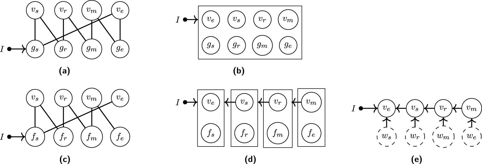
Bipartite graph: The equilibrium bipartite graphs associated with the equilibrium equations of the filling bathtub, the viral infection, and the reaction network with feedback are given in Figure 5(a), (b), and (c), respectively. We have added also a node representing the input signal. The dynamic bipartite graphs for the dynamics of these models are constructed from first-order differential equations in canonical form^[14] in the following way. Both the derivative X ˙ i ( t ) and the corresponding variable X i ( t ) are associated with the same vertex v i . The natural labelling is used for the differential equations, so that a vertex g i is associated with the differential equation for X ˙ i ( t ) . We then construct the dynamic bipartite graph ℬ dyn = ⟨ V , F , E ⟩ with variable vertices v i ∈ V and the corresponding dynamical equation vertices g i ∈ F . Additional static equation vertices f i ∈ F are added as well in case the dynamical system consists of a combination of dynamic and static equations. The edge set E has an edge ( v i − f j ) whenever X i ( t ) appears in the static equation f j . In addition, there are edges ( v i − g j ) whenever X i ( t ) or X ˙ i ( t ) appears in the dynamic equation g j (which includes the cases i = j due to the natural labelling used). The dynamic bipartite graphs for the bathtub model, the viral infection, and the reaction network with feedback are given in Figure 5(d), (e), and (f), respectively.

Figure 5

Graphical representations of the bathtub model (left column), the viral infection model (center column), and the reaction network with negative feedback (right column). The input vertices I K , I σ , and I are represented by black dots, while exogenous variables are indicated by dashed circles. For each model, the structure of the equilibrium equations can be read off from the equilibrium bipartite graphs in (a)–(c). The structure of the first-order differential equations can be represented with the dynamic bipartite graphs in (d)–(f). The equilibrium causal ordering graphs corresponding to the equilibrium bipartite graphs are given in (g)–(i). Similarly, the dynamic causal ordering graphs corresponding to the dynamic bipartite graphs can be found in (j)–(l). The equilibrium Markov ordering graphs for the equilibrium distribution of the models are given in (m)–(o).

Comparing the equilibrium bipartite graphs with the dynamic bipartite graphs we note that there is no edge ( v D − f D ) in Figure 5(a), while ( v D − g D ) is present in Figure 5(d). This is a direct consequence of the fact that the time derivative X ˙ D ( t ) in equation (4) does not depend on X D ( t ) itself. Similarly, the edges ( v I − f I ) and ( v E − f E ) are not present in Figure 5(b), whilst the edges ( v I − g I ) and ( v E − g E ) are present in Figure 5(e). In this case, we see that even though the time derivatives X ˙ I ( t ) and X ˙ E ( t ) depend on X I ( t ) and X E ( t ) in differential equations (12) and (13), these variables do not appear in the associated equilibrium equations (15) and (16). Finally, there is no edge ( v B − f B ) in Figure 5(c), while the edge ( v B − g B ) is present in Figure 5(f). Here, the variable X B ( t ) does not appear in the equilibrium equation under saturation conditions (20) that stems from the dynamic equation (18) for X ˙ B ( t ) . The equilibrium bipartite graph can be compared to the dynamic bipartite graph to read off structural differences between the equations before and after equilibrium has been reached.

Causal ordering graph: The application of the causal ordering algorithm to the equilibrium bipartite graphs of the filling bathtub, the viral infection, and the reaction network results in the equilibrium causal ordering graphs in Figure 5(g), (h), and (i), respectively. Henceforth, we will assume that the dynamic bipartite graph has a perfect matching that extends the natural labelling of the dynamic equations, i.e., such that all pairs ( v i , g i ) are matched. Application of the causal ordering algorithm to the associated dynamic bipartite graph for the model of a filling bathtub, the viral infection model, and the reaction network results in the dynamic causal ordering graphs in Figure 5(j), (k), and (l), respectively.^[15]

As shown in ref. [12], the absence (presence) of a directed path from an equation vertex to a variable vertex in the equilibrium causal ordering graph indicates that a soft intervention targeting a parameter in that equation has no (a generic) effect on the value of that variable once the system has reached equilibrium again. Furthermore, the absence (presence) of a directed path from a cluster to a variable vertex in the equilibrium causal ordering graph indicates that a perfect intervention targeting the cluster has no (a generic) effect on the value of that variable once the system has reached equilibrium again. Notice that the variables v i in the equilibrium causal ordering graph do not always end up in the same cluster with the equilibrium equation f i of the natural labelling. For example, we see in Figure 5(g) that a soft intervention targeting the equilibrium equation f O (e.g., a change in the value of U 5 ) does not affect the value of the outflow rate X O at equilibrium (since there is no directed path from f O to v O ), even though f O was obtained from the dynamic equation for the time derivative of the outflow rate X O ( t ) . Similarly, targeting f I with a soft intervention in the viral infection model has no effect on X I at equilibrium and targeting f C in the reaction network model has no effect on the equilibrium distribution of X C .^[16] This suggests that the causal structure at equilibrium of perfectly adapted dynamical systems may differ from the transient causal structure. In the next section, we will use this idea to detect perfect adaptation from background knowledge and experimental data.

Equilibrium Markov ordering graph: As explained in Section 2.2, the Markov ordering graph is constructed from the causal ordering graph and includes exogenous variables. For the bathtub model, we let vertices w I , w 1 , … , w 5 represent the independent exogenous random variables U I , U 1 , … , U 5 that appear in the model. For the viral infection model, we let w T , w I , w E , and w β represent independent exogenous random variables d T , d I , d E , and β in equations (11), (12), and (13). Finally, for the reaction network with negative feedback, we let w A , w B , and w C represent the independent exogenous random variables k I A , k C B , and k A C , respectively. The equilibrium Markov ordering graphs for the filling bathtub model, the viral infection model, and the model of a reaction network with a negative feedback loop are given in Figure 5(m), (n), and (o), respectively.^[17] These equilibrium Markov ordering graphs can be used to read off conditional independences in the equilibrium distribution that are implied by the equilibrium equations of the model. For example, since v I is d -separated from v D given v P in the equilibrium Markov ordering graph in Figure 5(m), X I will be independent of X D given X P once the system has reached equilibrium. These independences can be tested for in equilibrium data by means of statistical conditional independence tests. These implied conditional independences can, for instance, be used in the process of model selection [16].

3.3 Existence and uniqueness of solutions

The causal ordering algorithm is a graphical tool that can be useful when solving a system of equations. It decomposes the question of existence and uniqueness of a “global” solution into several “local” existence and uniqueness problems corresponding to a partitioning of the equations. When a unique global solution exists for all possible joint values of the (independent) exogenous variables, this leads to both a causal semantics and a Markov property [12]. We argue here that these ideas can also be extended to include differential equations. We will illustrate this with the filling bathtub model. We start with the (conceptually simpler) equilibrium model, which solely contains static equations, before discussing what to do when dynamic equations are present.

The equilibrium equations (7)–(10) can be solved in steps by following the topological ordering of the clusters in the equilibrium causal ordering graph in Figure 5(g). First, use f I to solve for X I , resulting in X I = U I . Then, use f D to solve for X O , which results in X O = X I . Subsequently, use f O to solve for X P , yielding X P = X O U 5 I K . Finally, use f P to solve for X D , resulting in X D = X P g U 3 . By substitution, we obtain a global solution of the form

Since we obtain a unique solution of each equation for the target variable in terms of the other variables appearing in the equation, this procedure shows that there exists a unique global solution of the system of equations for any value of the exogenous variables U I , U 1 , U 2 , U 3 , U 4 , U 5 and any value of the input signal I K . Because of this, we obtain both a causal interpretation and a Markov property for the filling bathtub model at equilibrium as described in Section 3.2.

For the dynamic filling bathtub model, we can follow a similar procedure, but now the clusters may also contain differential equations. We can make use of the theory for the existence and uniqueness of solutions of ordinary differential equations. First, note that the dynamic bipartite graph reflects the structure of the static and dynamic equations once we rewrite the differential equations as integral equations. For example, for the time interval [ t 0 , t ] :

Rewriting the differential equations as integral equations has two advantages: (i) there is no need to introduce the derivatives as if they were (variation) independent processes; (ii) it makes the dependence on the initial conditions X D ( t 0 ) , X P ( t 0 ) , and X O ( t 0 ) explicit. Equations (3)–(6) describing the dynamical system can be solved in steps by following the topological ordering of the clusters in the dynamic causal ordering graph in Figure 5(j). First, solve f I for X I , resulting in X I ( t ) = U I . The cluster { g D , g P , g O , v D , v P , v O } has to be dealt with as a single unit, which means we have to solve the subsystem of three differential equations { g D , g P , g O } (i.e., equations (4)–(6)) for its solution with components ( X D ( t ) , X P ( t ) , X O ( t ) ) . By applying the Picard–Lindelöf theorem (see, e.g., [50]), one obtains that this subsystem has a unique solution on a time interval [ t 0 , ∞ ) for any initial condition ( X D ( t 0 ) , X P ( t 0 ) , X O ( t 0 ) ) , provided that X I ( t ) and I K ( t ) are continuous and that the input signal I K ( t ) is bounded. Thus, equations (3)–(6) have a unique global solution for any value of the exogenous variables U I , U 1 , U 2 , U 3 , U 4 , U 5 , any initial condition ( X D ( t 0 ) , X P ( t 0 ) , X O ( t 0 ) ) , and any continuous and bounded input signal I K ( t ) . The approach of [12] can in this way be extended to yield both a dynamic causal interpretation and a Markov property (by using the trick of [34] to interpret path-continuous stochastic processes as random variables).^[18]

Important to note here is that this explicit solution procedure shows that at equilibrium, the value of the input signal I K may affect the value of X D and X P , but cannot affect the values of X O and X I , while there can be transient effects of the input signal I K ( t ) on X D ( t ) , X P ( t ) , and X O ( t ) , but not on X I ( t ) . Furthermore, under appropriate local solvability conditions for each cluster, these observations can directly be read off from the (equilibrium and dynamic) causal ordering graphs.

4.1 Identification of perfect adaptation via causal ordering

The identification of perfect adaptation via causal ordering makes use of the causal semantics of the equilibrium causal ordering graph. The following lemma states that a change in the input signal has no effect on the value of a variable if there is no directed path from the input vertex to that variable in the equilibrium causal ordering graph.

To establish perfect adaptation, we assume that the presence of a directed path in the dynamic causal ordering graph implies the presence of a transient causal effect.

Intuitively, this assumption may seem plausible, as the presence of the directed path in the dynamic causal ordering graph implies that the input signal enters into the construction of the solution of the variable, as sketched in Section 3.3. Unless a perfect cancellation occurs, one then expects a generic effect on the solution some time after the change in the input signal. Assumption 1 can be seen as a consequence of a certain faithfulness assumption.^[19] We conjecture that this assumption is generically satisfied for a large class of dynamical systems (e.g., it might hold for almost all parameter values with respect to the Lebesgue measure on a suitable parameter space).^[20]

By combining Lemma 1 and Assumption 1, we immediately obtain the following result.

Theorem 1 can be directly applied to the equilibrium and dynamic causal ordering graphs in Figure 5 to identify perfect adaptation. For example, we see that there is a directed path from the input signal I K to v O in the dynamic causal ordering graph of the filling bathtub in Figure 5(j), while no such path exists in the equilibrium causal ordering graph in Figure 5(g). It follows from Theorem 1 that X O perfectly adapts to changes in the input signal I K . This is in agreement with the simulation in Figure 3(a). Similarly, we can verify that the amount of infected cells X I in the viral infection model perfectly adapts to changes in the input signal I σ and that X C perfectly adapts to I in the reaction network with negative feedback. Hence, perfect adaptation in the bathtub model, the viral infection model, and the reaction network with negative feedback can be identified by applying the graphical criteria in Theorem 1 to the respective causal ordering graphs. It is important to keep in mind, though, that what we can identify in this way is only the possibility of perfectly adaptive behaviour, relying on the implicit assumption that the system will actually equilibrate.

In Appendix D, we show that the sufficient conditions in Theorem 1 for the identification of perfect adaptation are not necessary. More specifically, we construct graphical representations for a dynamical model of a basic enzymatic reaction that achieves perfect adaptation but does not satisfy the conditions in Theorem 1. Interestingly, though, after rewriting the equations, the perfectly adaptive behaviour of these systems can be captured via Theorem 1. Further, in Appendix E, we show that the biochemical reaction network in Figure 4(b), which Ma et al. [17] identified as being capable of achieving perfect adaptation, does not satisfy the conditions in Theorem 1 either. We show that a change of variables enables one to still capture the perfectly adaptive behaviour of this system via Theorem 1.

4.2 Identification of perfect adaptation from data

So far we have only considered how perfect adaptation can be identified in mathematical models. In this section, we focus on methods for identifying perfect adaptation from data that are generated by perfectly adapted dynamical systems under experimental conditions. The most straightforward approach to detect perfect adaptation is to collect time-series data while experimentally changing the input signal to the system. One can then simply observe whether the variables in the system revert to their original values. However, this type of experimentation is not always feasible. Another way to identify feedback loops that achieve perfect adaptation uses a combination of observational equilibrium data, background knowledge, and experimental data. Our second main result, Theorem 2, gives sufficient conditions under which we can identify a system that is capable of perfect adaptation from experimental equilibrium data.

Theorem 2 applies in particular to experiments on the filling bathtub, viral infection, and chemical reaction systems (for the corresponding graphs, see Figure 5). For example, a soft intervention targeting f O in the bathtub example has no effect on the outflow rate at equilibrium X O , because there is no directed path from f O to v O in Figure 5(g), and an intervention targeting f C has no effect on the equilibrium concentration X C in the reaction network because there is no directed path from f C to v C in Figure 5(i). In both cases, the first condition of Theorem 2 is satisfied. For the viral infection model, we see that a soft intervention targeting f E has an effect on the amount of infected cells X I at equilibrium (since there is a directed path from f E to v I in Figure 5(h)), while there is no directed path from v E to v I in Figure 5(n). In this case, the second condition of Theorem 2 is satisfied.

We can devise the following scheme to detect perfectly adapted dynamical systems from data and background knowledge. The procedure relies on several assumptions, including d -faithfulness of the equilibrium distribution to the equilibrium Markov ordering graph. We start by collecting observational equilibrium data and use a causal discovery algorithm (such as LCD or FCI) to learn a (partial) representation of the equilibrium Markov ordering graph, assuming the observational distribution at equilibrium to be d -faithful with respect to the equilibrium Markov ordering graph. We then consider a soft intervention that changes a known equation in the first-order differential equation model (i.e., it targets a known equilibrium equation). If this intervention does not change the distribution of the variable corresponding to this target using the natural labelling, or if it changes the distribution of identifiable non-descendants of the variable corresponding to the target according to the learned Markov equivalence class, we can apply Theorem 2 to identify the dynamical system as being capable of perfect adaptation. This way, we could identify perfect adaptation in specific cases such as the filling bathtub, viral infection, and reaction network by exploiting a combination of background knowledge and experimental data. Another example of a possible application of Theorem 2 is given in Section 5.3.

5.1 Dynamical model

We adapt the mathematical model of [19] for the RAS-RAF-MEK-ERK signalling cascade, as in ref. [16].^[23] Let V = { v s , v r , v m , v e } be an index set for endogenous variables that represent the equilibrium concentrations X s , X r , X m , and X e of active (phosphorylated) RAS, RAF, MEK, and ERK proteins, respectively. We model their dynamics as follows:

where we assume that I ( t ) is an external stimulus or perturbation. Roughly speaking, there is a signalling pathway that goes from I ( t ) to X s ( t ) to X r ( t ) to X m ( t ) to X e ( t ) with negative feedback from X e ( t ) on X s ( t ) . As we did for the reaction network with negative feedback in Section 3.1.3, we will consider the system under certain saturation conditions. Specifically, for ( T e − X e ( t ) ) ≫ K m e and X e ( t ) ≫ K F e e , the following approximation holds:

We let f s , f r , f m , and f e represent the equilibrium equations corresponding to the dynamical equations in (25), (26), (27), and (29) respectively, where we assume the input signal to have a constant (possibly random) value I .

We simulated the model under these saturation conditions (picking values for K m e and K F e e close to zero) until it reached equilibrium, and then we recorded the changes in the concentrations X s ( t ) , X r ( t ) , X m ( t ) , and X e ( t ) after a change in the input signal I . The details of this simulation can be found in Appendix B. The results in Figure 3 show that active RAS, RAF, and MEK revert to their original values after an initial response, while the equilibrium value of active ERK changes. Apparently, the equilibrium concentrations X s , X r , and X m perfectly adapt to the input signal I , while the equilibrium concentration X e of active ERK depends on the input signal I .

5.2 Graphical representations

We consider graphical representations of the protein signalling pathway. By using the natural labelling, we construct the dynamic bipartite graph in Figure 7(a) from the first-order differential equations, with the input signal I included. The associated dynamic causal ordering graph is given in Figure 7(b).

Under saturation conditions, the equilibrium equations f s , f r , f m , and f e obtained by setting equations (25), (26), (27), and (29), respectively, to zero have the bipartite structure in Figure 7(c). Note that there is no edge ( f e − v e ) in the equilibrium bipartite graph because X E ( t ) does not appear in the approximation (29) of (28). The associated equilibrium causal ordering graph is shown in Figure 7(d), where the cluster { I } is added with an edge towards the cluster { v e , f s } because I appears in equation (25) and in no other equations. So far we have treated all symbols in equations (25)–(28) as deterministic parameters. Let w s , w r , w m , and w e represent independent exogenous random variables appearing in the equilibrium equations f s , f r , f m , and f e , respectively. After adding them to the causal ordering graph with edges to their respective clusters, we construct the equilibrium Markov ordering graph for the equilibrium distribution in Figure 7(e).

There is a directed path from the input vertex I to v s , v r , and v m in the dynamic causal ordering graph (Figure 7(b)), while the equilibrium causal ordering graph has no directed paths from I to v s , v r , or v m (Figure 7(d)). Under Assumption 1, we can apply Theorem 1 to conclude that X s , X r , and X m will perfectly adapt to a persistent change in the input signal I . This is in line with what we observed in the simulations (Figure 6).

Figure 6

Perfect adaptation in the model for the RAS-RAF-MEK-ERK signalling pathway. After an initial response to a change of the input signal from value I − = 1.0 to a value I + at time t = t 0 , the equilibrium concentrations of active RAS, RAF, and MEK revert to their original values, while the concentration of active ERK changes. Shown are concentrations of active RAS (a), RAF (b), MEK (c) and ERK (d) against time.

Figure 7

Five graphs associated with the protein signalling pathway model under saturation conditions where indices s , r , m , and e correspond to concentrations of active RAS, RAF, MEK, and ERK, respectively. (a) Dynamic bipartite graph. (b) Dynamic causal ordering graph. (c) Equilibrium bipartite graph. (d) Equilibrium causal ordering graph. (e) Equilibrium Markov ordering graph.

The d -separations in the equilibrium Markov ordering graph (Figure 7(e)) imply conditional independences between the corresponding variables at equilibrium. For example, from the graph in Figure 7(e), we read off the following (implied) conditional independences:

We verified that these conditional independences indeed appear in the simulated equilibrium distribution of the model (see Appendix C for details).

5.3 Inhibiting the activity of MEK

A common biological experiment that is used to study protein signalling pathways is the use of an inhibitor that decreases the activity of a protein on the pathway. Such an inhibitor slows down the rate at which the active protein is able to activate another protein. Here, we consider inhibition of MEK activity. We can model this as a change of the parameters of the differential equations in which X m ( t ) appears. We can interpret this experiment as a soft intervention on differential equation g e in the dynamic model and on equation f e at equilibrium, decreasing the rate k m e at which ERK is activated. Since there is a directed path from f e to v m , v r , v s , and v e in the equilibrium causal ordering graph in Figure 7(d), we expect that a change in an input signal I e on f e (e.g., a change in the parameter k m e in the case of the MEK inhibition) affects the equilibrium concentrations of active MEK, RAF, RAS, and ERK.

We assessed the effect of decreasing the activity of MEK on the equilibrium concentrations of RAS, RAF, MEK, and ERK. To that end, we simulated the perfectly adapted model (with parameters as described in Appendix B, in particular, k m e = 1.0 ) until it reached equilibrium. We then decreased the parameter that controls the activity of MEK to k m e = 0.98 . The recorded responses of the concentrations of active RAS, RAF, MEK, and ERK are displayed in Figure 8. From this, we confirm our prediction that inhibition of MEK activity affects the equilibrium concentrations of RAS, RAF, MEK, and ERK. A qualitative aspect of this change that one cannot read off from the graph is that the MEK inhibition increases (rather than decreases) the concentrations of active MEK, RAF, and RAS according to the model for this choice of the parameters.

Figure 8

Simulation of the response of the concentrations of active RAS, RAF, MEK, and ERK after inhibition of the activity of MEK. The system starts out in equilibrium with k m e = 1.0 . The concentrations of RAS, RAF, MEK, and ERK are recorded after the parameter controlling MEK activity is decreased to k m e = 0.98 from t = t 0 on.

Note that RAS, RAF, and MEK are non-descendants of ERK in the equilibrium Markov ordering graph in Figure 7(e), so that under the assumptions in Theorem 2, we could actually use this experiment to detect perfect adaptation in the protein pathway.

5.4 Testing model predictions on real-world data

In this subsection, we verify some of the predictions of the model we obtained in Sections 5.2 and 5.3 on real-world data. We will compare with predictions of the causal Bayesian network model proposed by ref. [18].

Figure 9 shows scatter plots for the (logarithms of) the expressions of active RAF, MEK, and ERK in the multivariate single-cell protein expression dataset that was used in ref. [18], for three (out of 14) different experimental conditions. The baseline condition (in blue) is the one where the cells were treated with anti-CD3 and anti-CD28, activators of the RAS-RAF-MEK-ERK signalling cascade. In another condition (in red), the cells were additionally exposed to U0126, a known inhibitor of MEK activity. By inspecting the scatter plots, we get a quick visual check of some of the predictions of the model. In particular, these plots clearly show that inhibition of MEK activity by administering U0126 results in an increase in the concentrations of active RAF and active MEK and a reduction in the concentration of active ERK. Furthermore, we clearly see a strong dependence between RAF and MEK (in both experimental conditions), but there is no discernible dependence between RAF and ERK or between MEK and ERK (in either experimental condition). In the light of the supposedly direct effect of MEK on ERK, it is surprising that the data show no significant dependence between the two.^[24] This apparent “faithfulness violation” is problematic for constraint-based causal discovery methods, as they will typically not identify the causal relation between MEK and ERK.

Figure 9

Scatter plots of the logarithms of active RAF, MEK, and ERK concentrations for the data in ref. [18]. The blue circles correspond to cells treated only with anti-CD3 and anti-CD28, which activate the signalling cascade. The red circles correspond to cells treated with anti-CD3, anti-CD28, and in addition, the MEK-activity inhibitor U0126. The inhibition of MEK results in an increase of MEK and RAF, whereas ERK is reduced. The black circles correspond to cells treated with β 2cAMP (but not anti-CD3 and anti-CD28), which seems to affect MEK, but leaves RAF and ERK invariant.

According to ref. [18], the biological consensus (at the time) was that there is a signalling pathway from RAF to MEK to ERK.^[25] They propose to model this pathway as a causal Bayesian network RAF → MEK → ERK , and this is also the structure identified by their causal discovery algorithm. That model predicts that inhibiting the MEK activity can only affect ERK. In Table 1, we summarize some of the observations made using the scatter plots in Figure 9, and whether they are in line with the predictions of the models (our perfectly adaptive model on the one hand, and the causal Bayesian network model on the other hand). We conclude that the predictions of the perfectly adaptive model are more in agreement with the data than those of the causal Bayesian network model.

Still, the perfectly adaptive model does not explain all aspects of the data. For example, the effects of the β 2cAMP stimulation (black circles in Figure 9) are hard to explain with either model. β 2cAMP is an AMP analogue that is supposed to activate the RAS-RAF-MEK-ERK cascade by promoting active RAS. It seems counterintuitive that this would lead to a strong reduction of active MEK in comparison to the activation of the cascade by means of anti-CD3 and anti-CD28, while leading to the same levels of active RAF and ERK. For completeness, in Table 2, we have indicated for all 12 perturbations in ref. [18] the effects on the levels of active RAF, MEK, and ERK. It appears questionable whether a simple causal model (such as the perfectly adaptive model) could account for all the observed perturbation effects.

5.5 Caveats for causal discovery

Experiments in which the protein signalling network is perturbed in various ways are of crucial importance to obtaining a causal understanding of the system. While very sophisticated causal discovery algorithms are available, we will here illustrate the key concepts by means of applying one of the simplest causal discovery algorithms based on conditional independences to equilibrium data from the model. We simulate the system in two different conditions, a baseline and a condition where the activity of MEK has been inhibited.

Consider observational equilibrium data from the protein signalling pathway model and also experimental equilibrium data from a setting where the MEK activity is inhibited. We introduce a context variable C that in this case simply indicates for each sample whether a MEK inhibition was applied. Because the decision whether to apply the MEK inhibitor to a sample occurs before the measurement, the equilibrium concentrations measured afterwards cannot causally affect this decision. Hence, C is an exogenous variable, i.e., it is not caused by other observed variables. This motivates the use of the LCD algorithm, which requires the existence of such a variable. For the MEK inhibition, the context variable represents a (soft) intervention on the equation f e in the equilibrium causal ordering graph in Figure 7(d). The equilibrium Markov ordering graph that includes the context variable C (but where the independent exogenous random variables have been marginalized out) is given in Figure 10(a). To construct this graph, the context variable C is first added to the equilibrium causal ordering graph in Figure 7(d) as a singleton cluster with an edge towards the cluster { v m , f e } . The equilibrium Markov ordering graph is then constructed from the resulting directed cluster graph in the usual way. From Figure 10(a), we can read off (conditional) independences to find the LCD triples that are implied by the equilibrium equations of the model. We find that our model implies the following LCD triples: ( C , v m , v r ) , ( C , v m , v s ) , ( C , v m , v e ) , ( C , v r , v s ) , ( C , v r , v e ) , and ( C , v s , v e ) . We verified this by explicit simulation (details in Appendix C).

Figure 10

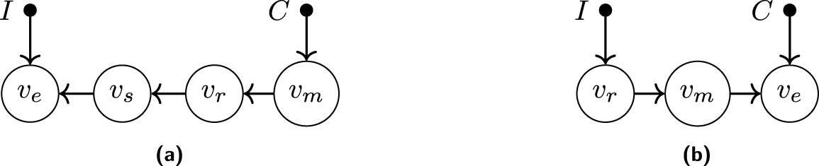
Equilibrium Markov ordering graphs of the protein signalling pathway with the context variable C included, corresponding to two hypothetical models. This context variable indicates whether a cell was treated with a MEK inhibitor or not. (a) Perfectly adaptive model (with feedback). (b) Causal Bayesian network model.

In particular, one of the LCD triples we obtained is ( C , v m , v r ) , whereas the triple ( C , v r , v m ) does not qualify as such. According to the standard interpretation of causal discovery algorithms, this would imply that MEK causes RAF rather than the other way around (see also Section 2.1), a surprising finding in the light of the textbook treatments of the RAS-RAF-MEK-ERK signalling pathway, and the “consensus network” according to ref. [18]. The equilibrium Markov ordering graph corresponding to the causal Bayesian network model of [18] is shown in Figure 10(b). As one can see from Figure 10(b), the causal Bayesian network model implies no LCD triples at all.

References

[1] Cooper GF. A simple constraint-based algorithm for efficiently mining observational databases for causal relationships. Data Min Knowl Discov. 1997;1:203–24. 10.1023/A:1009787925236Search in Google Scholar
[2] Richardson TS, Spirtes P. Automated discovery of linear feedback models. In: Gregory F. Cooper, Clark Glymour. Computation, Causation and Discovery. London, England: MIT Press; 1999. p. 253–302.10.7551/mitpress/2006.003.0010Search in Google Scholar
[3] Pearl J. Causality: models, reasoning, and inference. Cambridge, UK: Cambridge University Press; 2000. Search in Google Scholar
[4] Spirtes P, Glymour C, Scheines R. Causation, prediction, and search. Cambridge, Massachusetts: MIT Press; 2000. 10.7551/mitpress/1754.001.0001Search in Google Scholar
[5] Zhang J. On the completeness of orientation rules for causal discovery in the presence of latent confounders and selection bias. Artif Intell. 2008;172:1873–96. 10.1016/j.artint.2008.08.001Search in Google Scholar
[6] Hyttinen A, Eberhardt F, Hoyer PO. Learning linear cyclic causal models with latent variables. J Mach Learn Res. 2012;13(1):3387–439. Search in Google Scholar
[7] Colombo D, Maathuis MH, Kalisch M, Richardson TS. Learning high-dimensional directed acyclic graphs with latent and selection variables. Ann Stat. 2012;40:294–321. 10.1214/11-AOS940Search in Google Scholar
[8] Forré P, Mooij JM. Constraint-based causal discovery for non-linear structural causal models with cycles and latent confounders. In: Proceedings of the 34th Annual Conference on Uncertainty in Artificial Intelligence (UAI-18); 2018. p. 269–78. Search in Google Scholar
[9] Mooij JM, Magliacane S, Claassen T. Joint causal inference from multiple contexts. J Mach Learn Res. 2020;21:1–108. Search in Google Scholar
[10] Mooij JM, Claassen T. Constraint-based causal discovery using partial ancestral graphs in the presence of cycles. In: Proceedings of the 36th Conference on Uncertainty in Artificial Intelligence (UAI-20). vol. 124. Proceedings of Machine Learning Research (PMLR); 2020. p. 1159–68. Search in Google Scholar
[11] Simon HA. Causal ordering and identifiability. In: Studies in econometric methods. New York: John Wiley & Sons; 1953. p. 49–74. 10.1007/978-94-010-9521-1_5Search in Google Scholar
[12] Blom T, van Diepen MM, Mooij JM. Conditional independences and causal relations implied by sets of equations. J Mach Learn Res. 2021;22(178):1–62. Search in Google Scholar
[13] Iwasaki Y, Simon HA. Causality and model abstraction. Artif Intell. 1994;67:143–94. 10.1016/0004-3702(94)90014-0Search in Google Scholar
[14] Dash D. Restructuring dynamic causal systems in equilibrium. In: Proceedings of the Tenth International Workshop on Artificial Intelligence and Statistics (AIStats 2005); 2005. p. 81–8. Search in Google Scholar
[15] De Boer RJ. Which of our modeling predictions are robust? PLOS Comput Biol. 2012;8:e1002593. 10.1371/journal.pcbi.1002593Search in Google Scholar PubMed PubMed Central
[16] Blom T, Mooij JM. Robustness of model predictions under extension. In: Cussens J, Zhang K, editors. Proceedings of the Thirty-Eighth Conference on Uncertainty in Artificial Intelligence (UAI-22). vol. 180 of Proceedings of Machine Learning Research. PMLR; 2022. p. 213–22. Search in Google Scholar
[17] Ma W, Trusina A, El-Samad H, Lim WA, Tang C. Defining network topologies that can achieve biochemical adaptation. Cell. 2009;138:760–73. 10.1016/j.cell.2009.06.013Search in Google Scholar PubMed PubMed Central
[18] Sachs K, Perez O, Pe’er D, Lauffenburger DA, Nolan GP. Causal protein-signaling networks derived from multiparameter single-cell data. Science. 2005;308:523–9. 10.1126/science.1105809Search in Google Scholar PubMed
[19] Shin SY, Rath O, Choo SM, Fee F, McFerran B, Kolch W, et al. Positive- and negative-feedback regulations coordinate the dynamic behavior of the Ras-Raf-Mek-Erk signal transduction pathway. J Cell Sci. 2009;122:425–35. 10.1242/jcs.036319Search in Google Scholar PubMed
[20] Lauritzen SL, Dawid AP, Larsen BN, Leimer HG. Independence properties of directed Markov fields. Networks. 1990;20:491–505. 10.1002/net.3230200503Search in Google Scholar
[21] Lacerda G, Spirtes P, Ramsey J, Hoyer PO. Discovering cyclic causal models by independent components analysis. In: Proceedings of the 24th Annual Conference on Uncertainty in Artificial Intelligence (UAI-08); 2008. p. 1159–68. Search in Google Scholar
[22] Strobl EV. A constraint-based algorithm for causal discovery with cycles, latent variables and selection bias. Int J Data Sci Anal. 2019;8:33–56. 10.1007/s41060-018-0158-2Search in Google Scholar
[23] Bongers S, Forré P, Peters J, Mooij JM. Foundations of structural causal models with cycles and latent variables. Ann Stat. 2021;49(5):2885–915. 10.1214/21-AOS2064Search in Google Scholar
[24] Spirtes P. Directed cyclic graphical representations of feedback models. In: Proceedings of the 11th Annual Conference on Uncertainty in Artificial Intelligence (UAI-1995); 1995. p. 491–8. Search in Google Scholar
[25] Forré P, Mooij JM. Markov properties for graphical models with cycles and latent variables. 2017. arXiv:1710.08775v1 [math.ST]. https://arxiv.org/abs/1710.08775v1. Search in Google Scholar
[26] Richardson TS. Models of feedback: interpretation and discovery. PhD dissertation. Carnegie-Mellon University, 1996. Search in Google Scholar
[27] Nayak P. Automated modeling of physical systems. Berlin: Springer-Verlag; 1995. 10.1007/3-540-60641-6Search in Google Scholar
[28] Pothen A, Fan CJ. Computing the block triangular form of a sparse matrix. ACM Trans Math Softw. 1990;16:303–24. 10.1145/98267.98287Search in Google Scholar
[29] Gonçalves B, Porto F. A note on the complexity of the causal ordering problem. Artif Intell. 2016;238:154–65. 10.1016/j.artint.2016.06.004Search in Google Scholar
[30] Fisher FM. A correspondence principle for simultaneous equation models. Econometrica. 1970;38(1):73–92. 10.2307/1909242Search in Google Scholar
[31] Voortman M, Dash D, Druzdzel MJ. Learning why things change: the difference-based causality learner. In: Proceedings of the Twenty-Sixth Annual Conference on Uncertainty in Artificial Intelligence (UAI-10); 2010. p. 641–50. Search in Google Scholar
[32] Sokol A, Hansen NR. Causal interpretation of stochastic differential equations. Electr J Probabil. 2014;19:1–24. 10.1214/EJP.v19-2891Search in Google Scholar
[33] Rubenstein PK, Bongers S, Schölkopf B, Mooij JM. From deterministic ODEs to dynamic structural causal models. In: Proceedings of the 34th Annual Conference on Uncertainty in Artificial Intelligence (UAI-18); 2018. p. 114–23. Search in Google Scholar
[34] Bongers S, Blom T, Mooij JM. Causal modeling of dynamical systems. 2022 Mar. Preprint. arXiv:1803.08784v4 [cs.AI]. https://arxiv.org/abs/1803.08784v4. Search in Google Scholar
[35] Mogensen SW, Malinsky D, Hansen NR. Causal learning for partially observed stochastic dynamical systems. In: Proceedings of the 34th Annual Conference on Uncertainty in Artificial Intelligence (UAI-18); 2018. p. 350–60. Search in Google Scholar
[36] Mooij JM, Janzing D, Schölkopf B. From ordinary differential equations to structural causal models: the deterministic case. In: Proceedings of the 29th Annual Conference on Uncertainty in Artificial Intelligence (UAI-13); 2013. p. 440–8. Search in Google Scholar
[37] Lauritzen SL, Richardson TS. Chain graph models and their causal interpretations. J R Stat Soc Ser B (Stat Methodol). 2002;64:321–61. 10.1111/1467-9868.00340Search in Google Scholar
[38] Mooij JM, Janzing D, Heskes T, Schölkopf B. On causal discovery with cyclic additive noise models. Adv Neural Inform Process Syst (NIPS 2011). 2011;24:639–47. Search in Google Scholar
[39] Blom T, Bongers S, Mooij JM. Beyond structural causal models: causal constraints models. In: Proceedings of the 35th Uncertainty in Artificial Intelligence Conference (UAI-19). vol. 115 of Proceedings of Machine Learning Research; 2020. p. 585–94.Search in Google Scholar
[40] Dawid AP. Beware of the DAG! In: Proceedings of Workshop on Causality: Objectives and Assessment at NIPS 2008. vol. 6 of Proceedings of Machine Learning Research; 2010. p. 59–86. Search in Google Scholar
[41] Araujo RP, Liotta LA. The topological requirements for robust perfect adaptation in networks of any size. Nature Commun. 2018;9:29717141. 10.1038/s41467-018-04151-6Search in Google Scholar PubMed PubMed Central
[42] Muzzey D, Gómez-Uribe CA, Mettetal JT, van Oudenaarden A. A systems-level analysis of perfect adaptation in yeast osmoregulation. Cell. 2009;138:160–71. 10.1016/j.cell.2009.04.047Search in Google Scholar PubMed PubMed Central
[43] Ferrell JE. Perfect and near-perfect adaptation in cell signaling. Cell Sys. 2016;2:62–67. 10.1016/j.cels.2016.02.006Search in Google Scholar PubMed
[44] Krishnan J, Floros I. Adaptive information processing of network modules to dynamic and spatial stimuli. BMC Syst Biol. 2019;13:30866946. 10.1186/s12918-019-0703-1Search in Google Scholar PubMed PubMed Central
[45] Triantafillou S, Lagani V, Heinze-Deml C, Schmidt A, Tegner J, Tsamardinos I. Predicting causal relationships from biological data: applying automated causal discovery on mass cytometry data of human immune cells. Sci Rep. 2017;7:12724. 10.1038/s41598-017-08582-xSearch in Google Scholar PubMed PubMed Central
[46] Mooij JM, Heskes T. Cyclic causal discovery from continuous equilibrium data. In: Proceedings of the 29th Annual Conference on Uncertainty in Artificial Intelligence (UAI-13). Arlington, Virgina: AUAI Press; 2013. p. 431–9. Search in Google Scholar
[47] Ramsey J, Andrews B. FASK with interventional knowledge recovers edges from the Sachs model. 2018; arXiv:1805.03108 [q-bio.MN]. https://arxiv.org/abs/1805.03108. Search in Google Scholar
[48] Boeken PA, Mooij JM. A Bayesian nonparametric conditional two-sample test with an application to local causal discovery. In: Proceedings of the Thirty-Seventh Conference on Uncertainty in Artificial Intelligence (UAI-21). vol. 161 of Proceedings of Machine Learning Research; 2021. p. 1565–75. Search in Google Scholar
[49] Blom T, Klimovskaia A, Magliacane S, Mooij JM. An upper bound for random measurement error in causal discovery. In: Proceedings of the 34th Annual Conference on Uncertainty in Artificial Intelligence (UAI-18); 2018. p. 570–9. Search in Google Scholar
[50] Coddington EA, Levinson N. Theory of ordinary differential equations. New York: McGraw-Hill; 1955. Search in Google Scholar
[51] Meek C. Strong completeness and and faithfulness in Bayesian networks. In: Proceedings of the Eleventh Conference on Uncertainty in Artificial Intelligence (UAI-95); 1995. p. 411–8. Search in Google Scholar
[52] Sachs K, Itani S, Fitzgerald J, Schoeberl B, Nolan GP, Tomlin CJ. Single timepoint models of dynamic systems. Interface Focus. 2013;3:24511382. 10.1098/rsfs.2013.0019Search in Google Scholar PubMed PubMed Central
[53] Filippi S, Barnes CP, Kirk PD, Kudo T, Kunida K, McMahon SS, et al. Robustness of MEK-ERK dynamics and origins of cell-to-cell variability in MAPK signaling. Cell Reports. 2016 Jun;15:2524–35. 10.1016/j.celrep.2016.05.024Search in Google Scholar PubMed PubMed Central
[54] Fritsche-Guenther R, Witzel F, Sieber A, Herr R, Schmidt N, Braun S, et al. Strong negative feedback from Erk to Raf confers robustness to MAPK signalling. Mol Syst Biol. 2011;7(1):489. 10.1038/msb.2011.27Search in Google Scholar PubMed PubMed Central
[55] Chalupka K, Eberhardt F, Perona P. Causal feature learning: an overview. Behaviormetrika. 2017;44:137–67. 10.1007/s41237-016-0008-2Search in Google Scholar
[56] Murray JD. Mathematical biology I: an introduction. 3rd edition. New York: Springer-Verlag; 2002. 10.1007/b98868Search in Google Scholar
[57] Dash D, Druzdzel MJ. A note on the correctness of the causal ordering algorithm. Artif Intell. 2008;172:1800–8. 10.1016/j.artint.2008.06.005Search in Google Scholar
© 2023 the author(s), published by De Gruyter
This work is licensed under the Creative Commons Attribution 4.0 International License.
Articles in the same Issue
- Research Articles
- Adaptive normalization for IPW estimation
- Matched design for marginal causal effect on restricted mean survival time in observational studies
- Robust inference for matching under rolling enrollment
- Attributable fraction and related measures: Conceptual relations in the counterfactual framework