Heterogeneous interventional effects with multiple mediators: Semiparametric and nonparametric approaches

Max Rubinstein; Zach Branson; Edward H. Kennedy

doi:10.1515/jci-2022-0070

Article Open Access

Heterogeneous interventional effects with multiple mediators: Semiparametric and nonparametric approaches

Max Rubinstein , Zach Branson and Edward H. Kennedy

Published/Copyright: July 29, 2023

Published by

Become an author with De Gruyter Brill

Submit Manuscript Author Information

From the journal Journal of Causal Inference Volume 11 Issue 1

Abstract

We propose semiparametric and nonparametric methods to estimate conditional interventional indirect effects in the setting of two discrete mediators whose causal ordering is unknown. Average interventional indirect effects have been shown to decompose an average treatment effect into a direct effect and interventional indirect effects that quantify effects of hypothetical interventions on mediator distributions. Yet these effects may be heterogeneous across the covariate distribution. We consider the problem of estimating these effects at particular points. We propose an influence function-based estimator of the projection of the conditional effects onto a working model, and show under some conditions that we can achieve root-n consistent and asymptotically normal estimates. Second, we propose a fully nonparametric approach to estimation and show the conditions where this approach can achieve oracle rates of convergence. Finally, we propose a sensitivity analysis that identifies bounds on both the average and conditional effects in the presence of mediator-outcome confounding. We show that the same methods easily extend to allow estimation of these bounds. We conclude by examining heterogeneous effects with respect to the effect of COVID-19 vaccinations on depression during February 2021.

Keywords: mediation; heterogeneous effects; machine learning; nonparametrics; causal inference

MSC 2010: 62G08; 62P25; 62D20

1 Introduction

A goal of causal mediation analysis is to understand the mechanisms through which interventions work. “Natural effects” most directly pertain to the idea of mechanism [1] and decompose the individual-level treatment effect into pathways that work directly or via changes in mediator values. However, the identifying assumptions required to estimate these effects are unenforceable even in randomized experiments. These effects are also not generally identified in common applied settings that involve multiple mediators unless the mediators are considered jointly. “Interventional effects” were proposed as alternative causal estimands that are identifiable under weaker assumptions and in settings with multiple mediators [2,3]. These effects conceptualize hypothetical interventions on the mediator distributions defined at specific covariate values. Unlike natural effects, these effects are identifiable in a sequentially randomized experiment. While the relationship between interventional effects and mechanisms acting at an individual level is unclear [1], interventional effects have gained popularity in applied research over the past several years.

This popularity is also in part because the same statistical functionals yield alternative causal interpretations that are often of substantive interest. Specifically, under weaker assumptions, these same methods can quantify disparity reductions achieved via interventions on some possibly mediating factor(s). For example, Vansteelandt and Daniel [3] analyze disparities in breast-cancer survival among high and low socioeconomic status (SES) women. They consider a model where SES causes breast-cancer survival via a direct pathway and via cancer screening and treatment choices, so that SES takes the role of an exposure. They estimate that if low SES women had the same (conditional) distribution of cancer screening and treatment choices as high SES women, the observed disparity in breast-cancer survival between high and low SES women would be reduced by half. This effect requires conceiving of an unspecified hypothetical intervention that could shift the covariate-stratrum specific distributions of cancer screening and treatment choices among low SES women to match that of high SES women. However, this intervention does not require conceiving of potential outcomes with respect to SES, or more generally of the types of controversial counterfactual quantities required to conceive of natural effects [3].

To date, the literature on interventional effects has primarily focused on estimating average effects. We instead consider estimating conditional effects across covariates that are possibly continuous. For example, consider the application from [3]. One natural follow-up question might be how these disparity reductions change as a function of a woman’s age. Even if the total disparity in cancer survival were constant across age, it remains possible that age moderates the interventional effects and therefore also the proportion of the disparity that would be eliminated via such an intervention. These questions pertain to conditional interventional indirect effects (CIIEs). To our knowledge, proposed strategies to estimate the CIIE have been limited to parametric methods [3,4], and the validity of the inferences are tied to assumptions that the models are correctly specified.

Our first contribution is to propose methods that allow for flexible nonparametric and machine learning methods for estimation. Specifically, we consider the setting of a binary intervention and two discrete-valued mediators whose causal ordering is unknown. We propose two estimation procedures: first, a semiparametric projection-based approach; second, a fully nonparametric approach. Both procedures are conceptually simple, and involve a regression of an estimate of the uncentered influence function for the average effect onto the covariates. However, the semiparametric approach targets a projection of the CIIE onto a parametric model rather than the CIIE itself. Projection-based estimators have frequently been proposed in the context of different causal estimands [5–7]. Our proposal extends this idea to this setting, and we show that under some conditions, root-n consistent and asymptotically normal estimates of the projection parameter are possible. The second proposal considers a fully nonparametric estimation procedure (a “DR-Learner”) that targets the CIIE directly, extending results from ref. [8]. While directly targeting the CIIE instead of its projection may seem preferable, we cannot in general obtain root-n consistent estimates. Even so, we show that we can obtain oracle rates of convergence in some settings. Both the projection estimator and the DR-Learner substantially weaken the modeling assumptions used to date in the literature on estimating the CIIE. Moreover, these methods allow the use of flexible nonparametric and machine-learning methods for estimation while still obtaining relatively fast rates of convergence.

Our methods, like most, require several identifying assumptions, including that the mediator-outcome relationship is unconfounded. A natural question is whether our estimators are sensitive to violations of this assumption. We therefore derive bounds on the CIIE while relaxing this assumption and show that we can use both the projection-based approach and the DR-Learner to estimate these quantities. These methods naturally extend to allow for estimating bounds on the average effects, and we show that root-n consistent and asymptotically normal estimates of these bounds are possible under some conditions. Existing approaches frequently focus on the natural rather than interventional effects and are often tied to strong parametric modeling assumptions [9–11]. Moreover, sensitivity analyses for conditional estimands is less seldom discussed (though see ref. [12]).

Finally, we demonstrate these methods using an application previously considered in ref. [13]. This study sought to quantify the extent to which COVID-19 vaccines reduced self-reported depression via changes in social isolation versus worries about health among the COVID-19 Trends and Impact Survey (CTIS) respondents in February 2021. The authors only examined effect heterogeneity across discrete subgroups; moreover, they did not conduct a sensitivity analysis with respect to the interventional effect estimates. We revisit this analysis and model how the vote share for Joe Biden in the 2020 US presidential election in each respondent’s county of residence moderated the interventional effects. We then demonstrate our sensitivity analysis for the average and the CIIEs.

This article proceeds as follows. In Section 2, we review interventional effects, the required identifying assumptions, and efficient estimation. In Section 3, we introduce the CIIE and propose the projection-based estimator and the DR-Learner. We establish conditions required for asymptotic normality and root-n consistency of the projection estimator and for obtaining oracle rates of convergence for the DR-Learner. Section 4 contains a simulation study demonstrating that these theoretic properties hold in practice. Section 5 proposes our sensitivity analysis, Section 6 contains our application, and Section 7 contains a discussion of these results.

2 Review

We define the average interventional effects, the causal assumptions required to tie the causal targets to observed data, and efficient estimation of the observed data functionals. We largely summarize material covered in refs [3,14] and refer to those articles for more details. We begin by outlining the setup and notation that we will use throughout.

2.1 Setup and notation

Assume that we observe n i.i.d. samples of observations Z i = ( V i , W i , M 1 i , M 2 i , A i , Y i ) , where Y represents some outcome of interest (either continuous or discrete), A represents a binary intervention, and M 1 and M 2 represent discrete-valued mediators. Finally, we let [ V , W ] represent a matrix of either discrete or continuous covariates, where W may be empty, and which we jointly denote as X . We distinguish between V and W because we will estimate effects conditional on V = v , which may or may not include all elements of X . Figure 1 illustrates the assumed relationships between the variables, with an arrow indicating a causal pathway. Importantly, we do not assume that we know the causal relationship between M 1 and M 2 .

Figure 1

Assumed data generating process.

While this figure helps to motivate the problem, we will primarily rely on potential outcomes notation to define our assumptions. Specifically, we use Y a m 1 m 2 to denote potential outcomes under A = a , M 1 = m 1 , and M 2 = m 2 , and M j a to denote the counterfactual outcome for the j th mediator under A = a . For any discrete variable C , we use p ( c ) as a short hand for P ( C = c ) throughout.

We also define the following functions of the data. Let π a ( X ) = p ( A = a ∣ X ) and μ a ( M 1 , M 2 , X ) denote the outcome regression E [ Y ∣ A = a , X , M 1 , M 2 ] . We denote the joint mediator probabilities as p ( M 1 , M 2 ∣ X , A ) , and the marginal probabilities as p ( M 1 ∣ X , A ) and p ( M 2 ∣ X , A ) . Following the notation in ref. [14], we define the marginalized outcome models:

μ a , M 1 ( M 2 , X ) = ∑ m 1 μ a ( m 1 , M 2 , X ) p ( m 1 ∣ a , X ) μ a , M 1 × M 2 ′ ( X ) = ∑ m 1 , m 2 μ a ( m 1 , m 2 , X ) p ( m 1 ∣ a , X ) p ( m 2 ∣ a ′ , X ) .

These quantities are defined with respect to marginalizing the outcome regression over p ( M 1 ∣ a , X ) . We use this same notation to define quantities marginalized with respect to p ( M 1 ∣ a ′ , X ) (e.g., μ a , M 1 ′ × M 2 ′ ( X ) ).

We also denote sample averages using P n ( Z ) and regression estimates as E ˆ n ( Y ∣ X ) . For possibly random functions f , we denote ‖ f ‖ 2 as the squared L 2 ( P ) norm, ∫ f ( z ) 2 d P ( z ) . We use the notation a ≲ b to indicate that a ≤ C b for some universal constant C . Finally, for any random function f ˆ learned on an independent sample of size n , D 1 n , we let P f ˆ ( Z ) = ∫ f ˆ ( z ) d P ( z ∣ D 1 n ) . That is, P f ˆ ( Z ) refers to the expected value of this estimated function conditional on the training sample, noting that for a fixed function f this is equivalent to E ( f ) .

2.2 Interventional effects

We can decompose the average effect ψ = E [ Y a − Y a ′ ] into the sum of the following quantities [3]:

(1) ψ IDE = E ∑ m 1 , m 2 E [ Y a m 1 m 2 − Y a ′ m 1 m 2 ∣ X ] p ( M 1 a ′ = m 1 , M 2 a ′ = m 2 ∣ X ) ,

(2) ψ M 1 = E ∑ m 1 , m 2 E [ Y a m 1 m 2 ∣ X ] { p ( M 1 a = m 1 ∣ X ) − p ( M 1 a ′ = m 1 ∣ X ) } p ( M 2 a ′ = m 2 ∣ X ) ,

(3) ψ M 2 = E ∑ m 1 , m 2 E [ Y a m 1 m 2 ∣ X ] { p ( M 2 a = m 2 ∣ X ) − p ( M 2 a ′ = m 2 ∣ X ) } p ( M 1 a = m 1 ∣ X ) ,

(4) ψ Cov = E ∑ m 1 , m 2 E [ Y a m 1 m 2 ∣ X ] { p ( M 1 a = m 1 , M 2 a = m 2 ∣ X ) − p ( M 1 a = m 1 ∣ X ) p ( M 2 a = m 2 ∣ X ) − [ p ( M 1 a ′ = m 1 , M 2 a ′ = m 2 ∣ X ) − p ( M 1 a ′ = m 1 ∣ X ) p ( M 2 a ′ = m 2 ∣ X ) ] } ) .

The interventional direct effect ( ψ IDE ) represents the contrast in mean potential outcomes when we set A = a for everyone in the population versus A = a ′ , while drawing the mediators randomly for each individual from their counterfactual joint distribution under A = a ′ given subject-specific covariates X . By contrast, the interventional indirect effect via M 1 ( ψ M 1 ) holds A fixed at a for all individuals, and considers the average contrast between giving everyone subject-specific values of M 1 drawn randomly from the counterfactual distribution under A = a versus the distribution under A = a ′ given covariates X , and simultaneously drawing M 2 from the counterfactual distribution under A = a ′ given covariates X . The interventional indirect effect through M 2 ( ψ M 2 ) is defined analogously. The covariant effect ( ψ Cov ) is the difference between the total effect and all three of these effects and captures the effect of the dependence of the mediators on each other. This decomposition also holds switching the role of a and a ′ : Vansteelandt and Daniel [3] index these estimands by a to make this distinction, while for conceptual simplicity, we do not. In addition, for the purposes of this article we focus on effects via M 1 ; however, our proposed methods can be used for any of these estimands.

2.3 Identification

The estimands defined earlier require knowledge about the potential outcomes under each treatment and mediator value for each subject. However, for any individual, we do not observe all of these quantities. We therefore make the following identifying assumptions to connect these causal quantities to the observed data distribution. First, we assume consistency, where for a ⋆ ∈ { a , a ′ } and any ( m 1 , m 2 ) :

Assumption 1

(Consistency)

A = a ⋆ ⇒ ( M 1 , M 2 ) = ( M 1 a ⋆ , M 2 a ⋆ ) A = a ⋆ , M 1 = m 1 , M 2 = m 2 ⇒ Y = Y a ⋆ m 1 m 2 .

Consistency precludes the potential outcomes for any individual from depending on another individual’s treatment or mediator assignment. We next assume sequential ignorability:

Assumption 2

(Sequential ignorability)

(5) Y a ⋆ m 1 m 2 ⊥ A ∣ X ,

(6) ( M 1 a ⋆ , M 2 a ⋆ ) ⊥ A ∣ X ,

(7) Y a ⋆ m 1 m 2 ⊥ ( M 1 , M 2 ) ∣ ( A = a ⋆ , X ) .

Sequential ignorability consists of three assumptions: equations (5) and (6), or Y–A and M–A ignorability, state that A is independent of Y a ⋆ m 1 m 2 and ( M 1 a ⋆ , M 2 a ⋆ ) given X . Equation (7), or Y-M ignorability, states that ( M 1 , M 2 ) is independent of Y a ⋆ m 1 m 2 given X and A = a ⋆ . We next assume positivity:

Assumption 3

(Positivity)

(8) P ( min a ⋆ π a ⋆ ( X ) > ε ) = 1 , P ( min m 1 , m 2 , a ⋆ p ( m 1 , m 2 ∣ a ⋆ , X ) > ε ) = 1 , ε > 0 .

Equation (8) implies that the propensity scores are bounded away from zero and one and the joint mediator probabilities are bounded away from zero with probability one.^[1] Under these assumptions, we can write ψ M 1 in terms of the observed data distribution.

(9) ψ M 1 = E ∑ m 1 , m 2 μ a ( X , m 1 , m 2 ) { p ( m 1 ∣ X , a ) − p ( m 1 ∣ X , a ′ ) } p ( m 2 ∣ X , a ′ ) = E ( ψ M 1 ( X ) ) .

The functional in (9) reflects other interesting causal parameters under weaker assumptions. For example, consider the case where (7) holds but (5) and (6) do not. This situation is frequently relevant in cases where we are using interventional indirect effects to understand disparities and A is an indicator of some subgroup of interest (e.g., Black versus white individuals). In that case, (9) still targets the causal contrast:

(10) E ∑ m 1 , m 2 E [ Y m 1 m 2 ∣ a , X ] [ p ( m 1 ∣ a , X ) − p ( m 1 ∣ a ′ , X ) ] p ( m 2 ∣ a ′ , X ) .

This estimand tells us about how much an intervention on the distribution of M 1 could reduce an observed disparity in some outcome of interest [3]. However, in practice, we must carefully consider the relevant conditioning sets when defining these quantities [15].

2.4 Estimation

Regardless of the targeted causal quantity, (9) reflects a statistical parameter that is a fixed function of the observed data and we require methods to estimate this quantity. One natural idea would be to estimate each function in (9) separately, plug them into that same expression, and take the empirical average. If we were to use correctly specified parametric models to estimate the nuisance functions, the resulting estimate would be consistent for ψ M 1 and converge at n − 1 ∕ 2 rates. Unfortunately, this is unlikely to occur in practice. We could instead estimate these functions flexibly using nonparametric models; however, the subsequent estimator will in general inherit the nonparametric rate of convergence of the slowest estimated nuisance function, a rate generally slower than n − 1 ∕ 2 [16]. A different estimation strategy instead utilizes the so-called influence curve of (9). Influence curves are important quantities related to statistical functionals that naturally suggest efficient estimators without parametric modeling assumptions [16].

For example, ref. [14] previously showed that ψ M 1 has the efficient influence curve φ ( Z ; η ) − ψ M 1 , where the uncentered influence curve φ ( Z ; η ) takes the following form:

(11) φ ( Z ; η ) = 1 ( A = a ) π a ( X ) { p ( M 1 ∣ a , X ) − p ( M 1 ∣ a ′ , X ) } p ( M 2 ∣ a ′ , X ) p ( M 1 , M 2 , ∣ a , X ) ( Y − μ a ( M 1 , M 2 , X ) ) + 1 ( A = a ) π a ( X ) { μ a , M 2 ′ ( M 1 , X ) − μ a , M 1 × M 2 ′ ( X ) } − 1 ( A = a ′ ) π a ′ ( X ) { μ a , M 2 ′ ( M 1 , X ) − μ a , M 1 ′ × M 2 ′ ( X ) } + 1 ( A = a ′ ) π a ′ ( X ) ( μ a , M 1 ( M 2 , X ) − μ a , M 1 × M 2 ′ ( X ) − ( μ a , M 1 ′ ( M 2 , X ) − μ a , M 1 ′ × M 2 ′ ( X ) ) ) + μ a , M 1 × M 2 ′ ( X ) − μ a , M 1 ′ × M 2 ′ ( X ) ,

and where

(12) η = [ p ( M 1 , M 2 ∣ a , X ) , p ( M 1 , M 2 ∣ a ′ , X ) , μ a ( M 1 , M 2 , X ) , π a ( X ) ] .

By using φ ( Z ) , we can construct the so-called one-step estimator of ψ M 1 :

(13) ψ ˆ M 1 o s = P n [ φ ( Z ; η ˆ ) ] .

This estimator involves estimating η , plugging these estimates into (11) yielding φ ( Z ; η ˆ ) and taking the empirical mean. As shown in ref. [14], the following conditions are sufficient for this estimator to yield root-n consistent and asymptotically normal estimates.

The estimates η ˆ are obtained via sample splitting.
‖ φ ( Z ; η ˆ ) − φ ( Z ; η ) ‖ 2 = o p ( 1 ) .
‖ η ˆ − η ‖ = o p ( n − 1 ∕ 4 ) .

Condition (1) can be enforced in the estimation procedure. Condition (2) requires that the mean-squared error of the estimated influence-function converges in probability to zero at any rate. This would require, for example, that the propensity scores and their estimates be bounded away from zero and one, the joint mediator probabilities p ( m 1 , m 2 ∣ a , x ) and their estimates are bounded away from zero, and that the nuisance estimates η ˆ are consistent at any rate for η . Finally, condition (3) holds for a variety of nonparametric estimators of η under structural assumptions on the underlying nuisance functions: for example, on their smoothness or sparsity.

Influence function-based estimators can therefore attain n − 1 ∕ 2 convergence rates without parametric modeling assumptions and allowing for nonparametric estimates of the nuisance parameters. Intuitively, the reason is that we can essentially ignore the nuisance estimation error – assuming that we estimate the nuisance functions well enough (condition (3)). The asymptotics then follow as if we had an oracle that gave us the fixed (but unknown) function φ ( Z ; η ) and we took the average [16]. This remarkable fact occurs because the error of influence function-based estimators is a function of the product of errors in the nuisance estimation. By contrast, standard methods are in general linear in the nuisance estimation. As a result, influence function-based estimators can tolerate relatively slow rates of convergence for the nuisance estimates (e.g. rates achieved by nonparametric methods) while still obtaining faster rates of convergence for the estimand itself. Analogous to results shown by [8] for estimating the conditional average treatment effect (CATE), we will next show that we can also leverage φ ( Z ; η ) to achieve relatively fast rates of convergence when estimating the CIIE.

3 Conditional effects

In contrast to the average effects ψ M 1 , we consider estimating the effect at a given point V = v , recalling that X = [ W , V ] , so that V is a subset of the covariates X . In a slight abuse of notation,^[2] we define this estimand as follows:

(14) ψ M 1 ( v ) = E ∑ m 1 , m 2 E [ Y a m 1 m 2 ∣ X ] { p ( M 1 a = m 1 ∣ X ) − p ( M 1 a ′ = m 1 ∣ X ) } p ( M 2 a ′ = m 2 ∣ X ) ∣ V = v

Under Assumptions (1)–(3), these parameters are identified in the observed data as follows:

(15) ψ M 1 ( v ) = E ∑ m 1 , m 2 μ a ( X , m 1 , m 2 ) { p ( m 1 ∣ X , a ) − p ( m 1 ∣ X , a ′ ) } p ( m 2 ∣ X , a ′ ) ∣ V = v

A natural question is how well we can estimate these effects. Noting that

E [ φ ( Z ; η ) ∣ V = v ] = ψ M 1 ( v ) ,

we can think of an “oracle” influence function-based estimator as providing a benchmark for comparison for any other CIIE estimate:

(16) E ˆ n [ φ ( Z ; η ) ∣ V = v ] .

Just as the “oracle” estimate of ψ M 1 would be an empirical average of the true influence function, we can think of (16) as a local average of the true influence function around the point V = v . As long as Assumption 3 holds, we expect that the rate of convergence of (16) provides a valid, though possibly unachievable, lower bound for the rate of convergence for any estimator of the CIIE. This follows from noting that the convergence rate of this estimator is equivalent, up to constants, of replacing μ a ( X , m 1 , m 2 ) with the potential outcomes Y a m 1 m 2 in the expression for ψ M 1 ( X ) , and regressing this quantity onto V . While the remaining discussion compares our estimators against the oracle estimate, we expect that the oracle rates provide, in some settings, the best possible (minimax optimal) rates of convergence.^[3]

At a high level, both ideas we propose – the projection-estimator and the DR-Learner – substitute the estimated influence function φ ( Z ; η ˆ ) for φ ( Z ; η ) into a regression model E ˆ n . A key difference between these approaches is that the projection-estimator uses a parametric model for the regression and targets a projection of the CIIE, while the DR-Learner instead uses a nonparametric model and targets the CIIE itself. For either approach, we show the conditions where the corresponding oracle rates are attainable, analogous to results derived in [8]. Importantly, the theoretic results assume that the nuisance estimates η ˆ are estimated on an independent sample from the regression estimate E ˆ n . We therefore refer to this as a “second-stage” regression, reflecting the ordering of these two procedures. We discuss both procedures more in the following sections.

3.1 Projection estimator

We first consider the case where the second-stage regression estimate E ˆ n ( ⋅ ∣ V = v ) is given by the parametric model g ( v ; β ) , where β is a finite-dimensional parameter that minimizes some loss function. Specifically,

(17) β = arg min β ˜ E [ w ( X ) ℓ { ψ M 1 ( X ) − g ( V ; β ˜ ) } ] .

Importantly, we need not assume ψ M 1 ( X ) = g ( V ; β ) for g ( v ; β ) to represent a meaningful target of inference. Under no assumptions about ψ M 1 ( X ) , β represents a population parameter that characterizes a projection of ψ M 1 ( X ) onto g ( V ; β ) . For simplicity, we focus on the case, where β minimizes the squared-error loss ( ℓ ( z ) = z 2 ). The weights w ( X ) can vary to prioritize different parts of the covariate space when defining the projection, though in the simplest case, we can take them to be uniform. This projection, while not necessarily representing the true parameter ψ M 1 ( v ) , can nevertheless represent a useful summary of this parameter. The interpretation of parametric models as defining projections is well known, though perhaps underappreciated, in applied statistics and is frequently used in more general settings when attempting to summarize characteristics of unknown data-generating processes [17,18].

To estimate this projection, we assume standard regularity conditions and differentiate equation (17) with respect to β to obtain the following moment condition:

(18) E ∂ g ( V ; β ) ∂ β w ( X ) { ψ M 1 ( X ) − g ( V ; β ) } ≔ Ψ ( β ; P ) = 0 .

As with the average effects, our estimation approach is again based on the influence curve of Ψ ( β ; P ) . This yields an estimating-equation stated formally in Proposition 1.

Proposition 1

Under a nonparametric model, the uncentered efficient influence curve for the moment condition Ψ ( β ⋆ ) at any fixed β ⋆ is given by

(19) ϕ ( Z ; β ⋆ , η ) = ∂ g ( V ; β ⋆ ) ∂ β w ( X ) ( φ ( Z ; η ) − g ( V ; β ⋆ ) ) .

This then suggests the estimator β ˆ that satisfies:

(20) P n ∂ g ( V ; β ˆ ) ∂ β w ( X ) ( φ ( Z ; η ˆ ) − g ( V ; β ˆ ) ) = 0

Theorem 1 shows the conditions required to obtain root-n consistent and asymptotically normal parameter estimates.

Theorem 1

Consider the moment condition E [ ϕ ( Z ; β 0 , η 0 ) ] = 0 evaluated at the true parameters ( β 0 , η 0 ) . Now consider the estimator β ˆ that satisfies P n [ ϕ ( Z ; β ˆ , η ˆ ) ] = 0 , where η ˆ is estimated on an independent sample. Assume that:

The function class { ϕ ( Z ; β , η ) : β ∈ R p } is Donsker in β for any fixed η .
‖ ϕ ( Z ; β ˆ , η ˆ ) − ϕ ( Z ; β 0 , η 0 ) ‖ = o p ( 1 ) .
The map β → P [ ϕ ( Z ; β , η ) ] is differentiable at β 0 uniformly in the true η , with nonsingular derivative matrix ∂ ∂ β P { ϕ ( Z ; β , η ) } ∣ β = β 0 = M ( β 0 , η ) , where M ( β 0 , η ˆ ) → p M ( β 0 , η 0 ) .

Then

β ˆ − β = − M − 1 [ P n − P ] ϕ ( Z ; β 0 , η 0 ) + O p ( T 1 n + T 2 n + T 3 n + T 4 n ) ,

where

T 1 n = ‖ μ ˆ a ( M 1 , M 2 , X ) − μ a ( M 1 , M 2 , X ) ‖ ‖ π a ( X ) − π ˆ a ( X ) ‖ , T 2 n = ‖ μ ˆ a ( M 1 , M 2 , X ) − μ a ( M 1 , M 2 , X ) ‖ [ ‖ p ( M 1 , M 2 ∣ a , X ) − p ˆ ( M 1 , M 2 ∣ a , X ) ‖ + ‖ p ( M 1 ∣ a , X ) − p ˆ ( M 1 ∣ a , X ) ‖ + ‖ p ( M 2 ∣ a ′ , X ) − p ˆ ( M 2 ∣ a ′ , X ) ‖ + ‖ p ( M 1 ∣ a ′ , X ) − p ˆ ( M 1 ∣ a ′ , X ) ‖ ] , T 3 n = ‖ π a ( X ) − π ˆ a ( X ) ‖ [ ‖ p ( M 1 ∣ a , X ) − p ˆ ( M 1 ∣ a , x ) ‖ + ‖ p ( M 1 ∣ a ′ , X ) − p ˆ ( M 1 ∣ a ′ , x ) ‖ + ‖ p ( M 2 ∣ a ′ , X ) − p ˆ ( M 2 ∣ a ′ , X ) ‖ ] , T 4 n = ‖ p ( M 2 ∣ a ′ , X ) − p ˆ ( M 2 ∣ a ′ , X ) ‖ [ ‖ p ( M 1 ∣ a , X ) − p ˆ ( M 1 ∣ a , X ) ‖ + ‖ p ( M 1 ∣ a ′ , X ) − p ˆ ( M 1 ∣ a ′ , X ) ‖ ] .

Suppose further that T 1 n + T 2 n + T 3 n + T 4 n = o p ( n − 1 ∕ 2 ) . Then the proposed estimator attains the nonparametric efficiency bound and is asymptotically normal with

(21) n ( β ˆ − β ) → d N ( 0 , M − 1 E [ ϕ ϕ ⊤ ] M − ⊤ ) .

This also implies that for any fixed value of V = v :

(22) n ( g ( v ; β ˆ ) − g ( v ; β ) ) → d N 0 , ∂ g ( v ; β ) ∂ β ⊤ M − 1 E [ ϕ ϕ ⊤ ] M − ⊤ ∂ g ( v ; β ) ∂ β .

Remark 1

The expression T 1 n + T 2 n + T 3 n + T 4 n is expressed in terms of separate estimates for the marginal probability p ( M 1 ∣ a , X ) and the joint probability p ( M 1 , M 2 ∣ a , X ) . However, in practice, the estimate of p ( M 1 ∣ a , X ) may come from a marginalized estimate of p ( M 1 , M 2 ∣ a , X ) ; similarly, the estimates of p ( M 1 ∣ a ′ , X ) and p ( M 2 ∣ a ′ , X ) may come from marginalized estimates of p ( M 1 , M 2 ∣ a ′ , X ) . In this case, these estimates of the marginal probabilities will inherit the same rate of convergence as the estimate of these joint probabilities evaluated at the worst-case value of m 2 for p ( M 1 ∣ a , X ) (and similarly for p ( M 1 ∣ a ′ , X ) and p ( M 2 ∣ a ′ , X ) ), allowing us to simplify the second-order expressions above. Such an estimation approach is reasonable if we believe that these functions have the same underlying complexity. On the other hand, if we believe that the marginal probabilities are less complex than the joint probabilities, we may instead wish to estimate each marginal probability separately.

Theorem 1 illustrates that if we can estimate the components of η (defined in (12)) quickly enough β ˆ will be root-n consistent for β and asymptotically normal. It also implies that we can obtain pointwise confidence intervals for g ( v ; β ˆ ) by using any consistent estimate of the variance of (22) and standard normal quantiles. One sufficient condition for this to hold would be that we are able to estimate all elements of η at rates of at least o p ( n − 1 ∕ 4 ) . This is attainable by many nonparametric regression models under some conditions [19]. Alternatively, we could allow for slower rates for some nuisance components while requiring faster rates for others. For example, we could allow that ‖ μ a − μ ˆ a ‖ = o p ( n − 1 ∕ 6 ) and all other components to be estimated at o p ( n − 1 ∕ 3 ) . Regardless, as we saw when reviewing estimating the average effect ψ M 1 in Section 2.4, these conditions would imply that the regression of φ ( Z ; η ˆ ) onto g ( V ; β ) is asymptotically equivalent to the oracle regression of φ ( Z ; η ) onto g ( V ; β ) . Intuitively, this is because the error induced by the nuisance estimation is decreasing at rates faster than n − 1 ∕ 2 . As with estimating ψ M 1 , this in turn follows because the bias of β ˆ is a function of the product of errors in the nuisance estimation, as shown in the statement of Theorem 1.

3.2 DR-Learner

In some applications, we may not be satisfied with a projection and may instead wish to directly estimate ψ M 1 ( v ) . We propose estimating this quantity using a nonparametric second-stage regression model, which we call a DR-Learner following [8]. Algorithm 1 provides specific details. We then analyze the DR-Learner and derive results analogous to those found in ref. [8], giving model-free error bounds for arbitrary first-stage estimators, which reveal that under some conditions, the DR-Learner is as efficient as an oracle estimator that regresses φ ( Z ; η ) onto V directly. Our results are similar to [8]: the primary difference is that we must consider the sums of products of errors between several more sets of nuisance functions.

Algorithm 1

Let ( D 1 n , D 2 n ) denote two independent samples of n observations of Z i .

Step 1: Nuisance training. Construct estimates of η using D 1 n
Step 2: Pseudo-outcome regression. Construct the pseudo-outcomes φ ( Z ; η ˆ ) and regress it onto covariates V in the test sample D 2 n , giving
(23) ψ ˆ M 1 d r ( v ) = E ˆ n { φ ( Z ; η ˆ ) ∣ V = v } .
Step 3: Cross-fitting (optional). Repeat Steps 1 and 2, swapping the roles of D 1 n and D 2 n . Use the average of the resulting two estimates as a final estimate of ψ M 1 ( v ) .

Remark 2

In practice, when implementing either the DR-Learner or the projection estimator, one may wish to use sample-split estimates of φ ( Z ; η ˆ ) and regress them onto V using the entire sample, rather than averaging two separate estimates as suggested in Step 3. However, our results do not provide theoretic guarantees for this approach.

Proposition 1 from [8] establishes general conditions where the error of a pseudo-outcome regression of f ˆ onto V and an oracle regression of f onto V are asymptotically equivalent. This result relies on an assumption on the “stability” of the second-stage estimator with respect to a distance measure d and the convergence in probability of f ˆ to f with respect to d . Intuitively, estimator stability requires that the second-stage error between the pseudo-outcome regression and the oracle estimator converges in probability to the conditional bias of the pseudo-outcome estimates at a rate determined by root mean square error (RMSE) of the oracle estimator.^[4] Theorem 2 of ref. [8] shows the conditions for the oracle efficiency of a DR-Learner for the CATE under a direct application of Proposition 1 from ref. [8], where f is the uncentered influence function for the average treatment effect (ATE). We use the same approach for the CIIE to obtain analogous results, formalized in Corollary 1.

Corollary 1

Define b ˆ ⋆ ( x ) = E { φ ˆ ( Z ) − φ ( Z ) ∣ D 1 n , X = x } ; in other words, b ˆ ⋆ ( x ) is the conditional bias of the estimated influence function at X = x conditional on the training data. Assume

E ˆ n is stable with respect to distance metric d ,
d ( φ ˆ , φ ) → p 0 .

Let ψ ˜ M 1 ( v ) denote an oracle estimator from a regression of the true efficient influence function onto V and K n ⋆ ( v ) denote the oracle RMSE, E [ { ψ ˜ M 1 ( v ) − ψ M 1 ( v ) } 2 ] 1 ∕ 2 . Then

(24) ψ ˆ M 1 d r ( v ) − ψ ˜ M 1 ( v ) = E ˆ n { b ˆ ⋆ ( X ) ∣ V = v } + o p ( K n ⋆ ( v ) ) .

We provide an expression for b ˆ ⋆ ( x ) in Section B of the supplemental materials. Moreover, b ˆ ⋆ ( x ) ≲ b ˆ ( x ) , where:

(25) b ˆ ( x ) = T 1 n ( x ) + T 2 n ( x ) + T 3 n ( x ) + T 4 n ( x )

and

T 1 n ( x ) = ( π ˆ a ( x ) − π a ( x ) ) ∑ m 1 , m 2 ( μ a ( m 1 , m 2 , x ) − μ ˆ a ( m 1 , m 2 , x ) ) T 2 n ( x ) = ∑ m 1 , m 2 ( μ a ( m 1 , m 2 , x ) − μ ˆ a ( m 1 , m 2 , x ) ) ( p ( m 1 , m 2 ∣ a , x ) − p ˆ ( m 1 , m 2 ∣ a , x ) + ( p ( m 1 ∣ a , x ) − p ˆ ( m 1 ∣ a , x ) ) + ( p ( m 1 ∣ a ′ , x ) − p ˆ ( m 1 ∣ a ′ , x ) ) + ( p ( m 2 ∣ a ′ , x ) − p ˆ ( m 2 ∣ a ′ , x ) ) ) T 3 n ( x ) = ( π a ( x ) − π ˆ a ( x ) ) ( p ( m 1 ∣ a , x ) − p ˆ ( m 1 ∣ a , x ) ) + ( p ( m 1 ∣ a ′ , x ) − p ˆ ( m 1 ∣ a ′ , x ) ) + ( p ( m 2 ∣ a ′ , x ) − p ˆ ( m 2 ∣ a ′ , x ) ) T 4 n ( x ) = ∑ m 1 , m 2 ( p ( m 2 ∣ a ′ , x ) − p ˆ ( m 2 ∣ a ′ , x ) ) ( ( p ( m 1 ∣ a , x ) − p ˆ ( m 1 ∣ a , x ) ) + p ( m 1 ∣ a ′ , x ) − p ˆ ( m 1 ∣ a ′ , x ) ) .

Therefore, the DR-Learner is oracle efficient if E ˆ n { b ˆ ( X ) ∣ V = v } = o p ( K n ⋆ ( v ) ) .

Remark 3

As with the second-order expression in Theorem 1, the expression for b ˆ ( x ) depends on products of errors with the marginal mediator probabilities; however, these estimates, as described in Algorithm 1, come from estimates of the joint mediator probabilities. The error in the marginal probabilities is therefore of the same order as the sums of the errors in the joint probabilities across the relevant mediator values. As noted in Remark 1, we may wish to estimate the marginal mediator probabilities separately if we believe that the underlying complexity of the marginal probabilities is simpler than the joint mediator probabilities, though such a situation may seem unlikely to occur in practice.

One interesting implication of Corollary 1 is that the rate of convergence is a function of the cardinality of the joint mediator values k . We can eliminate this dependence by invoking the following assumption:

Assumption 4

The smoothed product of errors between mediator probabilities and/or the outcome model are of the same order for any values of ( m 1 , m 2 ). For example, for any ( m 1 , m 1 ′ ) and ( m 2 , m 2 ′ ) ,

E ˆ n { ( p ( m 1 ∣ a , X ) − p ˆ ( m 1 ∣ a , X ) ) ( p ( m 2 ∣ a ′ , X ) − p ˆ ( m 2 ∣ a ′ , X ) ) ∣ V = v } = o p ( a n )

and

E ˆ n { ( p ( m 1 ′ ∣ a , X ) − p ˆ ( m 1 ′ ∣ a , X ) ) ( p ( m 2 ′ ∣ a ′ , X ) − p ˆ ( m 2 ′ ∣ a ′ , X ) ) ∣ V = v } = o p ( a n ) .

Assumption 4 would be reasonable if we do not believe the functional form of the mediator probabilities or outcome models varies in underlying complexity across different values of the mediators.

We next consider the form of the second-stage regression E ˆ n . Proposition 2 from [8] implies that when E ˆ n is a linear smoother of the form ∑ i w i ( v ; V n ) f ( Z i ) and ∑ i ∣ w i ( v ; V n ) ∣ = O p ( a n ) , and b ˆ ( x ) can be expressed in the form of b ˆ 1 ( x ) b ˆ 2 ( x ) , then

E ˆ n { b ˆ ( X ) ∣ V = v } = O p ( a n ‖ b ˆ 1 ‖ w , 2 ‖ b ˆ 2 ‖ w , 2 ) ,

where

‖ f ‖ w , 2 = ∑ i ∣ w i ( v ; V n ) ∣ ∑ j ∣ w j ( v ; V n ) ∣ ∣ f ( Z i ) ∣ 2 1 ∕ 2

Corollary 2 applies this result to Corollary 1.

Corollary 2

Assume the conditions of Corollary 1 and that E ˆ n is a minimax optimal linear smoother with ∑ i ∣ w i ( v ; V n ) ∣ = O p ( 1 ) . Notice that

b ˆ ( x ) = ∑ j b ˆ j 1 ( x ) b ˆ j 2 ( x ) ,

where j indexes all of the error products in (25). Therefore,

E ˆ n { b ˆ ⋆ ( X ) ∣ V = v } ≲ E ˆ n ∑ j b ˆ j 1 ( X ) b ˆ j 2 ( X ) ∣ V = v .

By Proposition 2 of [8], we then obtain that

E ˆ n { b ˆ ( X ) ∣ V = v } = ∑ j O p ( ‖ b ˆ j 1 ‖ w , 2 ‖ b ˆ j 2 ‖ w , 2 ) ≍ max j O p ( ‖ b ˆ j 1 ‖ w , 2 ‖ b ˆ j 2 ‖ w , 2 ) .

To make Corollary 2 concrete, consider the case, where K n ⋆ ( v ) = n − θ . This result implies that when the second-stage regression estimator is a linear smoother, the DR-learner will achieve the corresponding oracle rate when, for example, all of nuisance errors are at least o p ( n − θ ∕ 2 ) in the ‖ ⋅ ‖ w , 2 norm. More generally, the DR-Learner is oracle efficient as long as the highest order error product in (25) is o p ( n − θ ) in this same norm. Whether these rates are actually attainable in a given application depends on the underlying complexity of the nuisance functions.

4 Simulations

We verify that the expected performance of these estimation strategies corresponds with the theory outlined above using a simulation study. First, we outline the data-generating process; second, we demonstrate the performance of our proposed approaches on samples of size n = 1,000 when estimating the nuisance functions using SuperLearner [20]; finally, we compare the convergence rates of the DR-Learner versus a plugin approach while controlling the convergence rates of the nuisance estimation.

4.1 Setup

To illustrate our proposed approach, we conduct a simulation study with a one-dimensional covariate X (so that V = X ). Figure 2 illustrates the simulated nuisance functions as a function of X . One aspect of this setup is that the outcome models and the propensity score models have complexity unlikely to be fully captured by simple generalized linear models, motivating our use of nonparametric methods. A second aspect is that the implied function ψ M 1 ( X ) , illustrated in Figure 3, is less complex than these functions. We provide all details about the data-generating processes for our simulations, including the functions illustrated in Figure 2, in Section C of the supplemental materials. All code for the simulation studies is available online at https://github.com/mrubinst757/ciie.

Figure 2

Simulation: selected nuisance functions. Nuisance function specifications for simulation study.

Figure 3

Estimands. Total effects, indirect effects, and proportion mediated as a function of X .

Figure 3 also illustrates the implied curves of ψ M 2 ( X ) and ψ ( X ) , as well as the curves for the proportion mediated via each mediator (e.g., ψ M 1 ( X ) ∕ ψ ( X ) ). The effects are entirely mediated via M 1 and M 2 ,^[5] and the proportion mediated via M 1 increases with X .

4.2 Estimation: SuperLearner

We evaluate the performance of each estimator across 1,000 simulations on test samples of size 1000. To estimate the nuisance parameters we use SuperLearner, using both the “SL.glm” and “SL.ranger” libraries.^[6] These model our nuisance functions as a weighted combination of predictions from logistic regression and random forests models. After estimating the nuisance parameters using samples of size 1,000, we use a separate test sample to estimate the DR-Learner and projection estimators. We then predict the points at X = 0 and X = 2 .

While we expect both estimates to be consistent, the mean square error at each point should differ by constants: this is due to differing inverse weights in the expression for φ ( Z ) . Figure 1 in Section C of the supplemental materials illustrates the maximum possible inverse weight as a function of X : at X = 0 , the maximum weight is lowest, while at X = 2 , the maximum weight is highest. These two points arguably reflect the easiest and hardest parts of the covariate space to estimate, with the point where X = 2 reflecting a “worst-case scenario” in our simulation. As long as our assumptions hold, these weights do not affect the asymptotic results. However, they can affect their performance in finite samples, with higher variance estimates where the inverse weights are large. In addition, confidence intervals may have undercoverage, since their validity is also based on asymptotic approximations. Consequently, we expect the simulations to show better results when estimating the CIIE at X = 0 compared to X = 2 , also with possibly better coverage in these regions. More generally, this comparison highlights a key limitation of our proposed approach: in an actual sample, it may be challenging to estimate conditional effects where the inverse weights are extreme.

Table 1 considers the projection estimates and displays the bias, RMSE, and confidence interval coverage associated with our proposed approach (“Efficient”) and with a plugin approach that regresses plugin estimates of ψ M 1 ( x ) on the same model. Specifically, the plugin estimates involve estimating each component in the expression for ψ M 1 ( x ) and regressing these estimates, rather than estimates of φ ( Z ; η ) , onto g ( X ; β ) . We predict the projection at the points X ∈ { 0 , 2 } using either a linear or quadratic projection. While the plugin estimator has lower RMSE, the confidence interval coverage is close to zero. This reflects that the bias associated with the nuisance estimation does not converge quickly enough to zero, and we therefore cannot ignore the estimation error in the second-stage regression when conducting inference. By contrast, we obtain close to nominal coverage rates for the efficient estimator. Finally, as expected, the point X = 0 is easier to estimate than X = 2 , reflected by the fact that the RMSE is higher for estimates at X = 2 than X = 0 .

Table 1

Projection estimators: simulation performance, n = 1,000 (averaged over 1,000 simulations)

Point	Strategy	Projection	Truth	Bias	Std	RMSE	Coverage
0	Plugin	Linear	0.07	0.00	0.03	0.03	3.10
2	Plugin	Linear	0.11	− 0.04	0.02	0.04	1.00
0	Plugin	Quadratic	0.07	− 0.00	0.03	0.03	3.10
2	Plugin	Quadratic	0.11	− 0.04	0.02	0.05	0.80
0	Efficient	Linear	0.07	0.00	0.06	0.06	95.50
2	Efficient	Linear	0.11	− 0.00	0.08	0.08	93.80
0	Efficient	Quadratic	0.07	0.00	0.06	0.06	95.10
2	Efficient	Quadratic	0.11	0.00	0.10	0.10	93.50

Table 2 displays analogous results when using the DR-Learner to target the true CIIE rather than its projection.^[7] We use smoothing splines with the default tuning parameters for the second-stage regression,^[8] and use the variance estimates from the smoothing matrix and assume that the distribution of the estimates is asymptotically normal to generate confidence intervals. Table 2 shows that this procedure yields approximately nominal coverage rates.

Table 2

Nonparametric estimators: simulation performance, n = 1,000 (averaged over 1,000 simulations)

Point	Strategy	Truth	Bias	Std	RMSE	Coverage
0	DR-Learner	0.07	0.00	0.08	0.08	94.3
0	Plugin	0.07	− 0.00	0.03	0.03	—
2	DR-Learner	0.11	− 0.00	0.11	0.11	92.6
2	Plugin	0.11	− 0.04	0.03	0.05	—

As with the projection approach, the corresponding plugin approach has lower RMSE than the DR-Learner. This is likely a function of the inverse-probability weights associated with the DR-Learner, which could cause this result for a fixed sample size.

4.3 Estimation: convergence rates

We conclude by examining the convergence rates of the DR-Learner versus a plugin estimator by specifying the convergence rates of the nuisance estimation. Roughly, we add N ( C ∕ n α , C ∕ n 2 α ) to the true values of the nuisance parameters on the logistic scale to simulate estimates. By using these results, we construct “estimated” influence functions and regress them onto X using smoothing splines. In contrast to the simulation study above, we use these simulations to estimate the integrated mean square error across the entire domain of X . Figure 4 displays the results.

$Figure 4 Convergence of DR-Learner versus plugin and oracle estimators. Scaled RMSE of each estimation strategy as a function of sample size. “Slow” nuisance function is estimated O p ( n − 1 ∕ 10 ) {{\mathcal{O}}}_{p}\left({n}^{-1/10}) rates, remaining at O p ( n − 1 ∕ 2 ) {{\mathcal{O}}}_{p}\left({n}^{-1/2}) rates.$

Figure 4

Convergence of DR-Learner versus plugin and oracle estimators. Scaled RMSE of each estimation strategy as a function of sample size. “Slow” nuisance function is estimated O p ( n − 1 ∕ 10 ) rates, remaining at O p ( n − 1 ∕ 2 ) rates.

The y -axis displays the RMSE of each estimator scaled by n , while the x -axis displays the sample sizes. The top left panel considers the case where we set α = 0.5 for all nuisance parameters. The other panels instead set α = 0.1 for the function indicated in the panel title. As expected, when all nuisance functions are estimated at the same rate, the plugin estimator converges at the same rate as the DR-Learner. However, once one of the nuisance functions is estimated slowly, the plugin estimator converges more slowly (illustrated by the diverging green lines), while the DR-Learner appears to attain the oracle rates of convergence in all settings. We again observe that despite the slower convergence rates, the plugin estimator has lower RMSE than either the DR-Learner or oracle estimators in some settings.

In Section C of the supplemental materials, we present additional results where we estimate the CIIE as a proportion of the corresponding CATE. We outline two general approaches to this problem: first, where we estimate the CIIE and the CATE and take the ratio of these estimates; second, where we derive the influence function for the mean of the ratio and regress this onto V (this is similar to ref. [6], who consider estimating a conditional risk-ratio). Our simulations show that this quantity is quite difficult to estimate well due to the high variance of the estimators, although we are able to construct confidence intervals with approximately nominal coverage rates using either approach.

5 Sensitivity analysis

We next consider estimating ψ M 1 ( v ) when the assumption that the potential outcomes Y a m 1 m 2 are independent of the mediators given the covariates and that A = a does not hold. This might occur, for example, if there were a posttreatment confounder L that occurs prior to M but after A ; or, a pre-treatment confounder U that affects the Y–M relationship but not the A–M or A–Y relationships. We first outline a general sensitivity framework to generate bounds on the conditional or average effects while specifying the degree of these types of violations, where our approach builds from ref. [21]. We extend the projection estimator and DR-Learner to estimate bounds on the conditional effects, though our proposed method naturally also suggests influence function based estimators of the bounds on the average effects. These analyses can help an analyst assess how much inferences may change given a specified degree of confounding. We first briefly introduce additional assumptions and notation to ease exposition.

5.1 Setup and notation

First, we assume for simplicity that V = X ; that is, that the conditioning set is identical to the observed confounders, so that our target estimand is ψ M 1 ( x ) . Second, to construct a bound for ψ M 1 ( x ) , it will be helpful to write ψ M 1 ( x ) = ψ M 1 , a ( x ) − ψ M 1 , a ′ ( x ) , where:

ψ M 1 , a ( x ) = ∑ m 1 , m 2 E [ Y m 1 m 2 ∣ a , x ] [ p ( m 1 ∣ a , x ) ] p ( m 2 ∣ a ′ , x ) ψ M 1 , a ′ ( x ) = ∑ m 1 , m 2 E [ Y m 1 m 2 ∣ a , x ] [ p ( m 1 ∣ a ′ , x ) ] p ( m 2 ∣ a ′ , x ) .

Third, for any ( m 1 ′ , m 1 , m 2 ′ , m 2 ) , we let

E [ Y m 1 m 2 ∣ m 1 ′ , m 2 ′ , a , x ] = μ a m 1 m 2 ⋆ ( m 1 ′ , m 2 ′ , x ) .

Assuming that Y-M ignorability holds when it does not, we define the biased target of our estimator of ψ M 1 ( x ) :

ψ ¯ M 1 ( x ) = ψ ¯ M 1 , a ( x ) − ψ ¯ M 1 , a ′ ( v ) = ∑ m 1 , m 2 μ a ( m 1 , m 2 , x ) [ p ( m 1 ∣ a , x ) − p ( m 1 ∣ a ′ , x ) ] p ( m 2 ∣ a ′ , x ) .

Finally, to reduce notation, we let ( ⋅ ) indicate the arguments ( m 1 , m 2 , x ) .

While we focus the remaining discussion on the case where V = X , all of these results also hold at a point V = v by averaging the relevant quantities over the distribution p ( W ∣ V = v ) , recalling that X = [ V , W ] .

5.2 Sensitivity framework

The bias ψ ¯ M 1 ( x ) − ψ M 1 ( x ) occurs because for any ( m 1 , m 2 , x ) , in general E [ Y m 1 m 2 ∣ a , x ] ≠ μ a ( ⋅ ) . We first consider this bias of the outcome regression. Proposition 2 shows that we can bound this bias as a function of μ a ( ⋅ ) and a sensitivity parameter τ . We consider a general framework where the meaning of τ changes based on the chosen sensitivity analysis; however, we describe the interpretation of this parameter under each assumption below.

Proposition 2

Assume that we know some functions b l ( ⋅ ; τ ) and b u ( ⋅ ; τ ) parameterized by τ such that for every ( m 1 , m 2 , x ) :

b u ( ⋅ ; μ a , τ ) ≥ μ a m 1 m 2 ⋆ ( M 1 ≠ m 1 , M 2 ≠ m 2 , x ) − μ a ( ⋅ ) ≥ b l ( ⋅ ; μ a , τ )

This implies the following bounds:

b u [ ⋅ ; μ a , τ ] [ 1 − p ( m 1 , m 2 ∣ a , x ) ] ≥ E [ Y m 1 m 2 ∣ a , x ] − μ a ( ⋅ ) ≥ b l [ ⋅ ; μ a , τ ] [ 1 − p ( m 1 , m 2 ∣ a , x ) ] .

Different assumptions on the selection process can motivate different functions b l and b u . For example, let τ ( m 1 , m 2 , x ) ∈ [ 0 , 1 ] . Consider the following three assumptions for any ( m 1 ′ ≠ m 1 ) and ( m 2 ′ ≠ m 2 ) :

(26) τ ( ⋅ ) ≥ ∣ μ a m 1 m 2 ⋆ ( m 1 ′ , m 2 ′ , x ) − μ a ( ⋅ ) ∣ ,

(27) τ ( ⋅ ) + μ a ( ⋅ ) [ 1 − τ ( ⋅ ) ] ≥ μ a m 1 m 2 ⋆ ( m 1 ′ , m 2 ′ , x ) ≥ ( 1 − τ ( ⋅ ) ) μ a ( ⋅ ) ,

(28) 1 ∕ ( 1 − τ ( ⋅ ) ) ≥ μ a m 1 m 2 ⋆ ( m 1 ′ , m 2 ′ , x ) ∕ μ a ( ⋅ ) ≥ ( 1 − τ ( ⋅ ) ) .

Under Assumption 26, τ bounds the absolute value of the difference between the regression functions μ a m 1 m 2 ⋆ ( m 1 ′ , m 2 ′ , x ) and μ a ( ⋅ ) for each level of ( m 1 , m 2 , x ) . Under assumption 28, τ parameterizes deviations of these same regression functions on the risk-ratio scale: below by 1 − τ , and above by 1 1 − τ .^[9] Finally, the meaning of τ changes for the upper and lower bound under assumption 27. First, the lower bound is equivalent to the lower bound in assumption 28, and τ retains an equivalent meaning in this case. However, the upper bound instead specifies that ( 1 − μ a m 1 m 2 ⋆ ( m 1 ′ , m 2 ′ , x ) ) ∕ ( 1 − μ a ( ⋅ ) ) ≥ ( 1 − τ ( ⋅ ) ) . Under this assumption, τ parameterizes the risk ratio of the regression function when the event Y did not occur.^[10] We discuss the trade offs between these assumptions in greater detail below.

While these assumptions provide bounds on the true outcome model, they imply, but are not equivalent to, bounds on ψ M 1 ( x ) . Proposition 3 provides a generic form of these bounds.

Proposition 3

Consider assumptions (26)–(28) and a sensitivity parameter τ ( x ) that is valid for any value of ( m 1 , m 2 ) at the point X = x . All [ b l , b u ] implied by these assumptions can be expressed as follows:

[ b l , b u ] = [ ( c l μ a ( ⋅ ) + t l ) f l ( τ ( x ) ) , ( c u μ a ( ⋅ ) + t u ) f u ( τ ( x ) ) ]

for constants ( c l , c u , t l , t u ) ∈ { 0 , 1 } 4 and functions f l and f u . At a point X = x , this yields the following bounds on ψ M 1 ( x ) :

(29) ψ M 1 , u b ( x ; τ ) = [ ψ ¯ M 1 ( x ) + ψ ¯ M 1 , a ( x ) f u ( τ ) c u − ψ ¯ M 1 , a ′ ( x ) f l ( τ ) c l + t u f u ( τ ) − t l f l ( τ ) − f u ( τ ) ∑ m 1 , m 2 [ c u μ a ( m 1 , m 2 , x ) + t u ] p ( m 1 , m 2 ∣ a , x ) p ( m 1 ∣ a , x ) p ( m 2 ∣ a ′ , x ) + f l ( τ ) ∑ m 1 , m 2 [ c l μ a ( m 1 , m 2 , x ) + t l ] p ( m 1 , m 2 ∣ a , x ) p ( m 1 ∣ a ′ , x ) p ( m 2 ∣ a ′ , x ) ,

(30) ψ M 1 , l b ( x ; τ ) = [ ψ ¯ M 1 ( x ) + ψ ¯ M 1 , a ( x ) f l ( τ ) c l − ψ ¯ M 1 , a ′ ( x ) f u ( τ ) c u + t l f l ( τ ) − t u f u ( τ ) − f l ( τ ) ∑ m 1 , m 2 [ c l μ a ( m 1 , m 2 , x ) + t l ] p ( m 1 , m 2 ∣ a , x ) p ( m 1 ∣ a , x ) p ( m 2 ∣ a ′ , x ) + f u ( τ ) ∑ m 1 , m 2 [ c u μ a ( m 1 , m 2 , x ) + t u ] p ( m 1 , m 2 ∣ a , x ) p ( m 1 ∣ a ′ , x ) p ( m 2 ∣ a ′ , x ) .

Remark 4

If we desired bounds at the point V = v , we could choose a τ valid for any realization of W at the point V = v and average these expressions over the conditional distribution of W given V = v . If we desired bounds on the average effect, we could choose a τ valid for all ( x , m 1 , m 2 ) and marginalize the aforementioned expressions over the entire covariate distribution.

The assumptions outlined in equations (26)–(28) yield different bounds. While (26) is perhaps most intuitive, for a given τ , the widths of the implied bounds on ψ M 1 in equations (29) and (30) are twice as large as those from (27) and are thus perhaps less useful in practice than the others. Comparing the assumptions in equations (27) and (28) is difficult: for a fixed τ , the scale of the confounding for the upper bounds of μ a m 1 m 2 ⋆ in these equations is simply different. One benefit of (28) is that it only requires reasoning about the risk ratio μ a m 1 m 2 ⋆ ( m 1 ′ , m 2 ′ , x ) ∕ μ a ( ⋅ ) . By contrast, (27) requires additional reasoning about the risk ratio bias in the estimates that the event Y did not occur, demanding more thought from the user. On the other hand, when using a binary outcome, equation (28) may result in an upper bound on μ a m 1 m 2 ⋆ greater than one, while equation (27), and the resulting bound on ψ M 1 ( x ) , will always respect the parameter space. Finally, for a fixed value of τ , it is unclear whether the bounds yielded by equations (27) or (28) will be wider. However, for fixed ( m 1 , m 2 , x ) , the upper bound on μ a m 1 m 2 ⋆ in (28) will always be larger than the bounds in (27) when μ a ( ⋅ ) ≥ 0.5 . Heuristically, we may therefore expect the bounds yielded by (28) to be narrower than those from (27) when μ a tends to be small across values of ( m 1 , m 2 , x ) . As a final point, the bound given by (27) is only useful for binary outcomes, or bounded outcomes rescaled to fall within 0 and 1, so that the sensitivity analysis given by (28) is more general.

Finally, we can extend this general approach in several ways. For example, Assumptions (26)–(28) yield similar bounds for ψ M 2 , ψ Cov , and ψ IDE by averaging over the relevant distributions. We discuss these extensions in Section E of the supplemental materials. We could also specify τ as a function that varies across ( m 1 , m 2 , x ) to arrive at a slightly different expression for the bounds. However, specifying this function would be challenging in practice.

5.3 Illustration

Figure 5 uses simulated data to illustrate the estimand, the biased target, and the bounds as a function of x choosing τ = 0.1 under (27) and τ = 0.15 under (28). These parameters reflect the true maximal values of τ guaranteed to hold under these assumptions in our simulation. We obtain biased estimates for our outcome model based on (27) and a parameter τ that varies between 0.1 ∗ { 1 ∕ 3 , 2 ∕ 3 , 1 } depending on the value of x . We describe the selection process in greater detail in Section C.4 of the supplemental materials. The upper and lower bounds are depicted in purple and red, while the orange and green lines reflect ψ ¯ M 1 ( x ) and ψ M 1 ( x ) , respectively. As x increases, the bounds given by (28) are at first narrower and eventually wider than the bounds given by (27). This is generally expected as the values of μ a ( m 1 , m 2 , x ) tend to increase with x (see Figure 3 in Section C of the supplemental materials). These bounds are also quite conservative: assuming (27), the bounds are only guaranteed to hold for all x for τ = 0.1 . However, even τ = 0.02 provides valid upper and lower bounds across the entire domain in our simulation. Of course, the gap between the value of τ guaranteed to hold and the minimum τ that actually does may be smaller for other data distributions; however, it does suggest that these bounds may be conservative in practice.

$Figure 5 Bounds on CIIE. Target estimand in green, biased target of inference in orange. Purple and red lines reflect upper and lower bounds that differ in terms of τ \tau specification.$

Figure 5

Bounds on CIIE. Target estimand in green, biased target of inference in orange. Purple and red lines reflect upper and lower bounds that differ in terms of τ specification.

5.4 Alternative approach

Tchetgen and Shpitser [22] and VanderWeele and Chiba [23] considered similar approaches for bounds on natural effects under the assumption that M–A and Y–A ignorability holds but that Y–M ignorability does not. Both proposals assume a known selection function that holds with equality rather than inequality. We could modify our proposed approach in a similar spirit. For example, we could assume that for all ( m 1 ′ ≠ m 1 ) , ( m 2 ′ ≠ m 2 ) :

μ a m 1 m 2 ⋆ ( m 1 ′ , m 2 ′ , x ) − μ a ( m 1 , m 2 , x ) = f ( τ ) [ c μ a ( m 1 , m 2 , x ) + t ] .

We could then recover ψ M 1 ( x ) (and any averages of it) exactly as follows:

ψ M 1 ( x ) = ψ ¯ M 1 ( x ) [ 1 + c f ( τ ) ] − c ∑ m 1 , m 2 μ a ( m 1 , m 2 , x ) p ( m 1 , m 2 ∣ a , x ) [ p ( m 1 ∣ a , x ) − p ( m 1 ∣ a ′ , x ) ] p ( m 2 ∣ a ′ , x ) − t f ( τ ) ∑ m 1 , m 2 p ( m 1 , m 2 ∣ a , x ) [ p ( m 1 ∣ a , x ) − p ( m 1 ∣ a ′ , x ) ] p ( m 2 ∣ a ′ , x ) .

While such an assumption would allow us to point identify ψ M 1 ( x ) , the concept requires knowledge about a selection function that we are unlikely to have. Despite the conservative inferences, we therefore prefer our proposed approach.

5.5 Estimation

We extend all of the aforementioned methods to estimate the bounds on ψ M 1 ( v ) . Theorem 3 in Section A.2 of the supplemental materials provides the expressions for the influence functions of the bounds on the average effect ψ M 1 . Equipped with this expression, we can again use a projection estimator or the DR-Learner to estimate the bounds.^[11] Intuitively, these approaches share the property that the upper bound on the convergence rates in the estimation is governed by the products of errors in the nuisance estimation. Corollaries 3 and 4 in Section A.2 of the supplemental materials give formal statements of these results using the lower bound as an example, although we can derive an upper bound analogously. We also provide expressions for the influence function for the bounds of ψ M 2 , ψ Cov , and ψ IDE in Section E of the supplemental materials and conjecture that results analogous to Corollaries 3 and 4 can be derived for these estimands. Finally, for a fixed τ , Theorem 4 in Section A.2 of the supplemental materials establishes the conditions where the one-step estimator for the bounds on the average effects is root-n consistent and asymptotically normal. We illustrate this estimation procedure in the application in Section 6.

6 Application

To demonstrate these methods, we revisit the data and application considered in [13], who examined the effect of COVID-19 vaccinations on depression, social isolation, and worries about health during February 2021 using the CTIS. The Delphi group at Carnegie Mellon University conducted the CTIS from April 2020 through June 2022 in collaboration with the Facebook Data for Good group [24]. By using these data, Rubinstein et al. [13] posit a model that COVID-19 vaccinations affect depression via a direct path, social isolation, and worries about health. By using the decomposition from ref. [3], they found that pathways via social isolation were more important than pathways via worries about health in explaining the effect of COVID-19 vaccinations on depression. We refer to that article for details on the data and the limitations of this analysis. While this study examined effect heterogeneity, the authors only examined heterogeneity within discrete subgroups and primarily focused on the outcomes analysis. Moreover, the authors did not find substantial effect heterogeneity with respect to the mediation analysis among the specified subgroups.

We examine the decomposition of the total effect within the following subset of CTIS respondents: employed, non-Hispanic, White respondents aged 25–54 years, with at least a college degree, no chronic health conditions, who work outside the home, and who had previously received an influenza vaccination. This included a total of 13,764 individuals. Table 3 displays the average effect estimates using influence function-based estimators, where the nuisance parameters were estimated using 20 stacked XGBoost models with different hyperparameter settings on the full dataset. While restricted to a much smaller subgroup, these results are qualitatively comparable to the average estimates in ref. [13].

Table 3

Average effect estimates on CTIS subset in February 2021, N = 13,764

Estimand	Estimate	Lower 95% CI	Upper 95% CI
Total effect	− 4.61	− 6.10	− 3.12
IIE - M1	− 1.86	− 2.45	− 1.28
IIE - M2	− 0.46	− 0.71	− 0.20
IIE - Cov	0.08	− 0.15	0.30
IDE	− 2.37	− 3.81	− 0.92

We next compare whether the interventional effects differed among those who live in counties where Trump led Biden by 50 percentage points in the 2020 election (“Trump counties”), and those where Biden led Trump by 50 percentage points (“Biden counties”). By limiting our sample to the subgroup defined earlier, effect heterogeneity across the Biden vote share may proxy for how social factors may moderate the mediated effects.^[12] Specifically, we hypothesize that these relatively educated, vaccine-accepting, and health conscious respondents who live in Trump-voting counties may have lower total effects than those who live in Biden areas due to the added stress of living in areas that generally took relatively fewer COVID precautions. We similarly hypothesize that the effects via worries about health might be lower in Trump-voting counties than Biden-voting counties for this same reason. Figure 6 displays the results using both the DR-Learner and projection estimators at these two points, where we use a simple linear model for the projection.^[13] Figure 4 in Section D of the supplemental materials display the entire estimated curves.

Figure 6

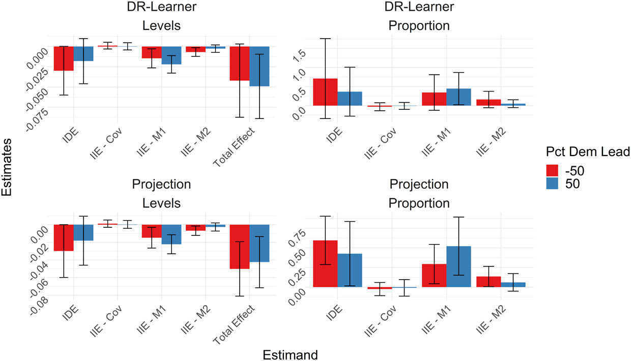
Application results. Conditional total, indirect, and direct effects in Biden (Pct Dem Lead = 50) versus Trump (Pct Dem Lead = − 50 ) counties.

The total effect estimates are comparable in the Trump counties relative to Biden counties; however, the projection estimates are slightly lower in Trump relative to Biden counties, while the DR-Learner suggests that these effects may be slightly higher.^[14] On the other hand, the effects via worries about health and social isolation are nearly identical for both the projection-estimator and DR-Learner. As shown in Figure 4 in Section D of the supplemental materials, the chosen smoothing parameter ends up essentially fitting a linear model for all functions other than the total effect. Regardless, the point estimates are consistent with our expectations, where effects via worries about health are lower in Trump counties relative to Biden counties. Meanwhile, effects via isolation appear slightly larger in Trump counties relative to Biden counties. However, all observed differences in these effects are small relative to the uncertainty estimates, and we are unable to draw statistically significant conclusions.

6.1 Sensitivity analysis

We conduct a sensitivity analysis for ψ M 1 both on average and as a function of Biden’s vote share. Figure 7 displays the results assuming (28) and where the conditional bounds are estimated using the DR-Learner.

$Figure 7 Bounds for application. Bounds for average and conditional interventional indirect effects via social isolation as a function of τ \tau .$

Figure 7

Bounds for application. Bounds for average and conditional interventional indirect effects via social isolation as a function of τ .

We find that that our average effect estimates are robust to a τ as large as 0.05, where τ parameterizes the deviations of the unobserved counterfactual regression function to the observed regression function on the risk ratio scale (equation (28)). In other words, if this ratio were less than 0.95 ( 1 − 0.05 ), or greater than 1.05 ( 1 1 − 0.05 ) for any value of ( x , m 1 , m 2 ) , our bounds would include a null effect. Our conditional effect estimates are less robust, in part due to the greater uncertainty estimates. For example, our estimates for Trump counties is robust only up to τ of 0.01 and for Biden counties is robust to τ of 0.03.

As a point of comparison, if we assumed that no unmeasured confounding held conditional on X , but we failed to control for any covariates, across all values of ( m 1 , m 2 ) , we would calculate a maximal τ = 0.95 . To be precise, we estimate that:

1 1 − 0.95 ≥ E [ Y m 1 m 2 ∣ A = a , M 1 ≠ m 1 , M 2 ≠ m 2 ] E [ Y m 1 m 2 ∣ A = a , M 1 = m 1 , M 2 = M 2 ] = E [ E [ Y ∣ A = a , M 1 = m 1 , M 2 = m 2 , X ] ] E [ Y ∣ A = a , M 1 = m 1 , M 2 = M 2 ] ≥ ( 1 − 0.95 ) ,

where the equality holds via assuming no unmeasured confounding conditional on X and consistency. Therefore, a set of unmeasured confounders with comparable association with the potential outcome regression would easily explain away our estimated effects, as we find that we would be unable to rule out a null effect at τ = 0.05 . In other words, our significant effect would disappear if there were some unmeasured confounder U that were at least approximately 5% (0.05 / 0.95) as associative with the outcome as our entire observed covariate set. However, this comparison might be best thought of as a “worst-case scenario,” as we estimate τ using all measured confounders and our covariate set is quite rich. Interesting future work would be to estimate different values of τ under different covariate subsets to obtain possibly less conservative ranges of τ . Sensitivity results for the remaining parameters are available in Section D of the supplemental materials.

7 Discussion

We propose two methods for estimating conditional average interventional indirect effects: a semiparametric projection-based approach and a fully nonparametric approach. These procedures are conceptually simple: regress an estimate of the uncentered influence function for the average parameter onto the desired covariates. The projection-based estimator uses a parametric regression model and therefore targets a projection of the CIIE, while the DR-Learner uses a fully nonparametric model for this regression, and therefore targets the CIIE itself. Our primary contribution is to establish the conditions where the convergence rates of these estimators are equivalent to that of an oracle regression of the true influence function onto these same models. As with estimating the CATE, the error of these estimators is a function of the product of errors in the nuisance estimation. However, unlike the CATE, we must consider the sums of several products of nuisance functions, which is in general a function of the cardinality of the joint mediators. While our discussion focused primarily on estimating the effect via M 1 , this approach can be extended to estimate other interventional effects, mediated effects, and likely a broad class of causal estimands.

As a second contribution, we propose a sensitivity analysis for the conditional effects that allows for mediator-outcome confounding. While the resulting bounds may be quite wide in practice, they make only weak assumptions on the underlying confounding mechanisms. Moreover, if one is willing to make stronger assumptions on the selection mechanism, more narrow bounds can be obtained using a slight variant of our approach. We propose a general approach to estimating these bounds using the projection estimators or DR-Learner, where our results are again not tied to any particular estimation method. Our methods also easily extend to estimating bounds on the average effects, allowing for root-n consistent and asymptotically normal estimates under some standard conditions.

Our proposed methods have several limitations: first, we only consider two discrete mediators and a binary treatment. However, we could broaden this general approach for more complex settings. For example, we could likely allow for several mediators by regressing the corresponding influence functions derived by [14] onto V . Similarly, we could likely extend our results to allow for continuous mediators. This would require additional assumptions, including, for example, the boundedness of the joint mediator density. A complete treatment of this topic would be an interesting area for future research. On the other hand, allowing for a continuous treatment would be a more challenging problem as the causal estimands themselves would have to be redefined, and an influence-function for the average effect does not exist. A second limitation of our proposed method is that our sensitivity analysis provides bounds that may be conservative. This is in part a function of the fact that the methods we considered are all with respect to worst-case scenarios that may occur infrequently in practice. A third limitation is that we do not study any number of other possible nonparametric estimation methods, such as an extension of the R-Learner proposed by ref. [25]. Finally, we do not explore the minimax optimal rates for CIIE estimation or propose estimators that might achieve these rates. Valuable future work could explore any of these questions.

Acknowledgments

The authors would like to thank Amelia Haviland for helpful discussions as this work developed. The authors would also like to thank the two anonymous reviews and the associate editor for helpful comments, questions, and suggestions that improved the quality of this article.

Funding information: The authors state no funding involved.
Conflict of interest: The authors state no conflict of interest.
Data availability statement: The data that support the findings of this study are available from https://dataforgood.facebook.com/dfg/docs/covid-19-trends-and-impact-survey-request-for-data-access but restrictions apply to the availability of these data, which were used under license for the current study, and so are not publicly available. Data are, however, available from the authors upon reasonable request and with permission of Facebook.

References

[1] Miles CH. On the causal interpretation of randomized interventional indirect effects. 2022. http://arXiv.org/abs/arXiv:220300245. 10.1093/jrsssb/qkad066Search in Google Scholar

[2] Didelez V, Dawid AP, Geneletti S. Direct and indirect effects of sequential treatments. In: Proceedings of the Twenty-Second Conference on Uncertainty in Artificial Intelligence; 2006. p. 138–46. Search in Google Scholar

[3] Vansteelandt S, Daniel RM. Interventional effects for mediation analysis with multiple mediators. Epidemiology (Cambridge, Mass). 2017;28(2):258. 10.1097/EDE.0000000000000596Search in Google Scholar PubMed PubMed Central

[4] Loh WW, Moerkerke B, Loeys T, Vansteelandt S. Heterogeneous indirect effects for multiple mediators using interventional effect models. Epidemiol Methods. 2020;9(1):20200023. 10.1515/em-2020-0023Search in Google Scholar

[5] Kennedy EH, Lorch S, Small DS. Robust causal inference with continuous instruments using the local instrumental variable curve. J R Stat Soc Ser B (Stat Meth). 2019;81(1):121–43. 10.1111/rssb.12300Search in Google Scholar

[6] Cuellar M, Kennedy EH. A non-parametric projection-based estimator for the probability of causation, with application to water sanitation in Kenya. J R Stat Soc Ser A (Stat Soc). 2020;183(4):1793–818. 10.1111/rssa.12548Search in Google Scholar

[7] Kennedy EH, Balakrishnan S, Wasserman L. Semiparametric counterfactual density estimation. 2021. http://arXiv.org/abs/arXiv:210212034. Search in Google Scholar

[8] Kennedy EH. Towards optimal doubly robust estimation of heterogeneous causal effects. 2020. https://arxiv.org/abs/2004.14497. Search in Google Scholar

[9] Park S, Qin X, Lee C. Estimation and sensitivity analysis for causal decomposition in health disparity research. Sociol Meth Res. 2022. 10.1177/00491241211067516 Search in Google Scholar

[10] Park S, Esterling KM. Sensitivity analysis for pretreatment confounding with multiple mediators. J Educ Behav Stat. 2021;46(1):85–108. 10.3102/1076998620934500Search in Google Scholar

[11] Imai K, Keele L, Tingley D. A general approach to causal mediation analysis. Psychol Meth. 2010;15(4):309. 10.1037/a0020761Search in Google Scholar PubMed

[12] Lindmark A, de Luna X, Eriksson M. Sensitivity analysis for unobserved confounding of direct and indirect effects using uncertainty intervals. Stat Med. 2018;37(10):1744–62. 10.1002/sim.7620Search in Google Scholar PubMed

[13] Rubinstein M, Haviland A, Breslau J. The effect of COVID-19 vaccinations on self-reported depression and anxiety during February 2021. Stat Public Policy. 2023;10(1):1–24. 10.1080/2330443X.2023.2190008. Search in Google Scholar

[14] Benkeser D, Ran J. Nonparametric inference for interventional effects with multiple mediators. J Causal Infer. 2021;9(1):172–89. 10.1515/jci-2020-0018Search in Google Scholar

[15] Jackson JW. Meaningful causal decompositions in health equity research: definition, identification, and estimation through a weighting framework. Epidemiology. 2020;32(2):282–90. 10.1097/EDE.0000000000001319Search in Google Scholar PubMed PubMed Central

[16] Kennedy EH. Semiparametric doubly robust targeted double machine learning: a review. 2022. http://arXiv.org/abs/arXiv:220306469. Search in Google Scholar

[17] Angrist JD, Pischke JS. Mostly harmless econometrics: an empiricistas companion. Princeton, NJ, United States: Princeton University Press; 2009. 10.1515/9781400829828Search in Google Scholar

[18] Buja A, Brown L, Berk R, George E, Pitkin E, Traskin M, et al. Models as approximations I: consequences illustrated with linear regression. Stat Sci. 2019;34(4):523–44. 10.1214/18-STS693Search in Google Scholar

[19] Tsybakov AB. Introduction to nonparametric estimation. 2009. 10.1007/b13794. Search in Google Scholar

[20] Van der Laan MJ, Polley EC, Hubbard AE. Super learner. Statistical applications in genetics and molecular biology. 2007;6(1). 10.2202/1544-6115.1309.Search in Google Scholar PubMed

[21] Luedtke AR, Diaz I, van der Laan MJ. The statistics of sensitivity analyses. UC Berkeley Division of Biostatistics Working Paper Series. 2015. https://biostats.bepress.com/ucbbiostat/paper341.Search in Google Scholar

[22] Tchetgen EJT, Shpitser I. Semiparametric theory for causal mediation analysis: efficiency bounds, multiple robustness, and sensitivity analysis. Ann Stat. 2012;40(3):1816. 10.1214/12-AOS990Search in Google Scholar PubMed PubMed Central

[23] VanderWeele TJ, Chiba Y. Sensitivity analysis for direct and indirect effects in the presence of exposure-induced mediator-outcome confounders. Epidemiol Biostat Public Health. 2014;11(2):e9027. 10.2427/9027Search in Google Scholar PubMed PubMed Central

[24] Salomon JA, Reinhart A, Bilinski A, Chua EJ, LaMotte-Kerr W, Rönn MM, et al. The US COVID-19 Trends and Impact Survey: Continuous real-time measurement of COVID-19 symptoms, risks, protective behaviors, testing, and vaccination. Proc Nat Acad Sci. 2021;118(51):e2111454118. 10.1073/pnas.2111454118Search in Google Scholar PubMed PubMed Central

[25] Nie X, Wager S. Quasi-oracle estimation of heterogeneous treatment effects. Biometrika. 2021;108(2):299–319. 10.1093/biomet/asaa076Search in Google Scholar

Received: 2022-10-24

Revised: 2023-04-17

Accepted: 2023-05-25

Published Online: 2023-07-29

This work is licensed under the Creative Commons Attribution 4.0 International License.

Supplementary material

Articles in the same Issue

https://doi.org/10.1515/jci-2022-0070

Keywords for this article

mediation; heterogeneous effects; machine learning; nonparametrics; causal inference

Creative Commons

BY 4.0

Heterogeneous interventional effects with multiple mediators: Semiparametric and nonparametric approaches

Article

Abstract

1 Introduction

2 Review

2.1 Setup and notation

2.2 Interventional effects

2.3 Identification

Assumption 1

Assumption 2

Assumption 3

2.4 Estimation

3 Conditional effects

3.1 Projection estimator

Proposition 1

Theorem 1

Remark 1

3.2 DR-Learner

Algorithm 1

Remark 2

Corollary 1

Remark 3

Assumption 4

Corollary 2

4 Simulations

4.1 Setup

4.2 Estimation: SuperLearner

4.3 Estimation: convergence rates

5 Sensitivity analysis

5.1 Setup and notation

5.2 Sensitivity framework

Proposition 2

Proposition 3

Remark 4

5.3 Illustration

5.4 Alternative approach

5.5 Estimation

6 Application

6.1 Sensitivity analysis

7 Discussion

Acknowledgments

References

Supplementary Material

Articles in the same Issue

Articles in the same Issue

Articles in the same Issue