Robust inference for matching under rolling enrollment

2.1 Setting and notation

We observe n subjects. For each subject i in the study, we observe repeated measures ( Y i , t , X i , t ) for timepoints t = 1 , … , T , where Y i , t is an outcome of interest and X i , t is a vector of covariates. We also observe a time of treatment initiation T i for each subject, with T i ∈ { 1 , … , T } for subjects who receive treatment at some point and T i = ∞ for those who remain controls at all observed timepoints. We specify a burn-in period of length L − 1 during which no individuals are treated, i.e., T i ≥ L for all i (or allow treatment at t = 1 by setting L = 1 ). We denote the collection of repeated measures for each subject i , along with T i , as the trajectory O i .

For clarity, we focus on “instantaneous” effects of treatment, with outcomes measured immediately following treatment. Let Y i , t ( 0 ) be the potential outcome for unit i that would have been observed at time t if T i > t , and let Y i , t ( 1 ) be the potential outcome that would have been observed if T i = t . The finite sample average effect of treatment on the treated (ATT) is denoted by Δ :

Here, the D i variable is introduced as a convenient shorthand to indicate whether T i < ∞ . We assume that trajectories O i are sampled independently from some infinite population, although we do not assume independence of observations within the same trajectory. By defining expectation E ( ⋅ ) with respect to sampling from this population, we define the population ATT as Δ pop = E ( Δ ) . For future convenience, we also introduce a concise notation for conditional expectation (again, over the sampling distribution) of potential outcomes given no treatment through time t and the covariates observed in the previous L timepoints:

Throughout, we relax notation slightly by writing μ 0 ( X i , t ) to indicate conditional expectation given the L lagged values of X i directly preceding time t , inclusive.

The potential outcomes framework adopted here represents one of many possible framings for studies with rolling enrollment. Pimentel et al. [10] define potential outcomes as functions of the length of time since treatment initiation, while both Ben-Michael et al. [3] and Athey and Imbens [16] define them as functions of the time of treatment initiation for the subject in question. In principle, these alternate constructions are much richer than ours, allowing for much more general and complicated patterns of effects, but in practice, all these authors use simplifying assumptions or focus on estimands that reduce attention to at most two potential outcomes of interest for each individual at each timepoint. For example, both Pimentel et al. [10] and Ben-Michael et al. [3] allow for treatment effects to be measured at some follow-up time postdating the time of treatment rather than focusing on instantaneous effects, but since the length of follow-up is fixed in advance, only two potential outcomes ever need to be considered for each unit. Similarly, the “no anticipation” assumption of both Ben-Michael et al. [3] and Athey and Imbens [16] ensures that there is exactly one potential outcome of interest associated with the control condition for each individual, and the “invariance to history” assumption of Athey and Imbens [16] collapses distinctions among potential outcomes under treatment. As such, the results we present in the following sections extend easily to all the potential outcomes frameworks just described, making the appropriate substitutions for our Y i , t ( 1 ) and Y i , t ( 0 ) . While the potential outcomes framework of Imai et al. [7] is much more general than all the previously mentioned works in allowing subjects to revert from treatment back to control, our framing also extends easily to it in the special case when no exit from treatment is allowed.

2.2 Identification assumptions

Pimentel et al. [10] studied the following difference-in-means estimator in designs where each treated unit is matched to C control observations. M i t , j t ′ is an indicator for whether subject i at time t has been matched to subject j at time t ′ :

Pimentel et al. [10] show that this estimator is unbiased for the population ATT under the following conditions:

1. Exact matching: matched units share identical values for covariates in the L timepoints preceding treatment.

2. L -ignorability: conditional on the covariate history over the previous L timepoints and the absence of treatment before baseline, an individual’s potential outcome at a given time is independent of the individual’s overall treatment status. Formally,

   { T i < ∞ } ⊥ ⊥ Y i , t ( 0 ) ∣ T i > t − 1 , { X i , s } s = t − L + 1 t , ∀ i .

   Intuitively, this assumption prevents unobserved confounding that makes potential outcomes for treated subjects systematically different from those that remain controls even after accounting for information from a baseline period.

3. Timepoint agnosticism: mean potential outcomes under control do not differ for any instances with identical covariate histories at different timepoints. Formally, for any set of L covariate values X ,

   μ 0 t ( X ) = μ 0 t ′ ( X ) = μ 0 ( X ) for any 1 ≤ t , t ′ ≤ T .

   This assumption ensures that matching across time is reasonable by ruling out time trends other than those captured by time-varying covariates. For clarity, we drop the t superscript when discussing the conditional expectation μ 0 ( X ) in what follows, with the exception of Section 6 where we temporarily consider failures of this assumption.

4. Covariate L -exogeneity: future covariates do not encode information about the potential outcome at time t given covariates and absence of treatment over the previous L time points. Formally,

   ( X i , 1 , … , X i , T ) ⊥ ⊥ Y i , t ( 0 ) ∣ T i > t − 1 , { X i , s } s = t − L + 1 t , ∀ i .

   Like time agnosticism, covariate L -exogeneity is important to justify considering past and future instances from a control trajectory as part of the matching procedure. If future instances’ covariates include or are correlated with past instances’ outcomes, then we may indirectly match on study outcomes introducing bias into our estimation step [17,18]. Covariate L -exogeneity ensures that future covariates are safe to consider during the design stage.

5. Overlap: given that a unit is not yet treated at time t − 1 ≥ L , the probability of entering treatment at the next time point is neither 0 nor 1 for any choice of covariates over the L timepoints at and preceding t .

   0 < P ( T i = t ∣ T i > t − 1 , X i t , … , X i t − L + 1 ) < 1 ∀ t > L .

   While this assumption is not stated explicitly in the study by Pimentel et al. [10], we note that the authors rely on an overlap assumption of this type in the proof of their main result.

The exact matching assumption is no longer needed for asymptotic identification of the population ATT if we modify the estimator by adding in a bias correction term. As shown in the studies by Otsu and Rai [15] and Abadie and Imbens [19], we first estimate the conditional mean function μ 0 ( X ) of the potential outcomes and use this outcome regression to adjust each matched pair for residual differences in covariates not addressed by matching. As outlined in the study by Abadie and Imbens [19], bias correction leads to asymptotic consistency under regularity conditions on the potential outcome mean estimator μ ^ ( ⋅ ) (for further discussion of regularity assumptions on μ ^ 0 ( ⋅ ) see the proof of Theorem 1 in Section A of the supplemental appendix). Many authors have also documented benefits from adjusting matched designs using outcome models [20,21]. The specific form of our bias-corrected (i.e., model-adjusted) estimator is as follows:

Datasets with many variables, especially continuous variables or variables with many categories, ensure that exact matching is rarely possible in practice, and in light of this, we focus primarily on estimator Δ ^ adj in what follows.

As discussed by Imai et al. [7] for settings without rolling enrollment, identification is possible under weaker assumptions if a difference-in-differences estimator is used instead of the difference-in-means. While we focus primarily on the simpler bias-corrected difference-in-means estimator for clarity of exposition, the difference-in-differences approach also offers advantages for our setting, and the new matching and inference strategies we propose extend naturally to such estimators. We provide further discussion in Section 4.3.

4.1 Inference methods for matched designs

Broadly speaking, there are two schools of thought in conducting inference for matched designs. One approach, spearheaded by Abadie and Imbens [19,25–27], views the raw data as samples from an infinite population and demonstrates that estimators based on matched designs (which in this framework are considered to be random variables, as functions of random data) are asymptotically normal. Inferences are based on the asymptotic distributions of matched estimators. A second approach, described in detail in Rosenbaum [28,29] and Fogarty [30], adopts the perspective of randomization inference in controlled experiments. Conditional on the structure of the match and the potential outcomes, the null distribution of a test statistic over all possible values of the treatment vector is obtained by permuting values of treatment within matched sets. When matches are exact and unobserved confounding is absent, strong finite sample guarantees hold for testing sharp null hypotheses without further assumptions on outcome variables. Asymptotic guarantees for weak null hypotheses may be obtained too, assuming a sequence of successively larger finite populations [31]. Well-developed methods of sensitivity analysis are also available.

As described in the study by Pimentel et al. [10], while standard methods of inference may be applied to GroupMatch without replacement, in which control individuals contribute at most one unit to any part of the match, none have been adequately developed for GroupMatch with trajectory replacement, in which distinct matched sets may contain different versions of the same control individual. For randomization inference, the barrier appears to be quite fundamental, because permutations of treatment within one matched set can no longer be considered independently for different matched sets. In GroupMatch with trajectory replacement, a treated unit receives treatment at one time and appears in a match only once; if treatment is permuted among members of a matched set so that a former control now attains treatment status, what is to be done about other versions of this control unit that are present in distinct matched sets? We note that similar issues arise when contemplating randomization inference for general cross-sectional matching designs with replacement, and we are aware of no solutions for randomization inference even in this simpler case.

In contrast, the primary issue in applying sampling-based inference to GroupMatch designs with trajectory replacement is the unknown correlation structure for repeated measures from a single control individual. The literature on matching with replacement provides estimators for pairs that are fully independent [27] and for cases in which a single observation appears identically in multiple pairs [25], but not for the intermediate case of GroupMatch with trajectory replacement where distinct but correlated observations appear in distinct matched sets. These issues extend beyond the GroupMatch family to any matched design under rolling enrollment in which control trajectories contribute to multiple matched sets, including those of Witman et al. [6] and Imai et al. [7].

In what follows, we give formal guarantees for a sampling-based inference method appropriate for general matching designs under rolling enrollment suggested by Imai et al. [7], which generalizes a recent proposal of Otsu and Rai [15] for valid sampling-based inference of cross-sectional matched studies using the bootstrap. Although the bootstrap often works well for matched designs without replacement [32], naive applications of the bootstrap in matched designs with replacement have been shown to produce incorrect inferences as a consequence of the failure of certain regularity conditions [26]. Intuitively, if matching is performed after bootstrapping the original data, multiple copies of a treated unit will necessarily all match to the same control unit, creating a clumping effect not present in the original data. However, Otsu and Rai [15] arrived at an asymptotically valid bootstrap inference method for matching by bootstrapping weighted and bias-corrected functions of the original observations after matching rather than repeatedly matching from scratch in new bootstrap samples. We show that a similar bootstrap approach, applied to entire trajectories of repeated measures in a form of the block bootstrap, provides valid inference for matched designs under rolling enrollment. Note that in our formal results, we focus on GroupMatch with instance replacement as the most difficult case, since the designs of Witman et al. [6] and Imai et al. [7] may be understood as restricted special cases in which matching on time is exact.

4.2 Block bootstrap

To conduct inference under GroupMatch with trajectory or instance replacement, we propose a weighted block bootstrap approach. We rearrange the GroupMatch ATT estimator from Section 2 as follows, letting K M ( i , t ) be the number of times the instance at trajectory i and time t is used as a match.

Because different instances of the same control unit are correlated, we resample the trajectory-level quantities Δ ^ i rather than the instance-level quantities. Since the Δ ^ i are functions of the K M ( i , t ) weights in the original match, we do not repeat the matching process within bootstrap samples. In particular, we proceed as follows:

1. Fit an outcome regression μ ^ 0 ( ⋅ ) based on covariates in the previous L timepoints using only control trajectories.

2. Match treated instances to control instances using GroupMatch with instance replacement. Calculate matching weights K M ( i , t ) equal to the number of times the instance at time t in trajectory i appears in the matched design.

3. Calculate the model-adjusted ATT estimator Δ ^ adj .

4. Repeat B times:

   1. Randomly sample N elements Δ ^ ∗ with replacement from { Δ ^ 1 , … , Δ ^ N } .

   2. Calculate the bootstrap bias-corrected ATT estimator Δ ^ adj ∗ for this sample of trajectories as follows:

      Δ ^ adj ∗ = 1 N 1 ∑ i = 1 N Δ ^ i ∗ .

5. Construct a ( 1 − α ) confidence interval based on the α / 2 and 1 − α / 2 percentile of the Δ ^ adj ∗ -values calculated from the bootstrap samples.

This method is essentially a block bootstrap, very similar to the method proposed in Imai et al. [7]. Note that while the recipe given earlier uses the nonparametric bootstrap, it may easily be generalized to other approaches such as the wild bootstrap and the Bayesian bootstrap. In particular, consider rewriting Δ ^ adj ∗ in terms of a new set of random variables W 1 ∗ , … , W N ∗ that we denote the bootstrap weights:

To recover the nonparametric bootstrap, the bootstrap weights W i ∗ are chosen as Q i / N 1 , where Q i is the number of times subject i is selected when sampling with replacement; if the W i ∗ are chosen instead by sampling from a scaled Dirichlet or scaled two-point distribution, we obtain the Bayesian bootstrap and the wild bootstrap, respectively (see Otsu and Rai [15] for specifics). To adapt the step-by-step algorithm for these approaches, we draw W i ∗ s rather than Δ ^ ∗ s in step 4(a) and use (1) to calculate Δ ^ adj ∗ in step 4b.

Our main result given here shows the asymptotic validity of this approach. Several assumptions, in addition to Assumptions 2–5 in Section 2.2, are needed to prove this result. We summarize these assumptions verbally here, deferring formal mathematical statements to Section A.1 of the supplemental appendix. First, we require the covariates X i to be continuous with compact and convex support and a density both bounded and bounded away from zero. Second, we require that the conditional mean functions are smooth in X , with bounded fourth moments. In addition, we require that conditional variances of the treated potential outcomes and conditional variances of nontrivial linear combinations of control potential outcomes from the same trajectory are smooth and bounded away from zero. We also require that conditional fourth moments of potential outcomes under treatment and linear combinations of potential outcomes under control are uniformly bounded in the support of the covariates. We also make additional assumptions related to the conditional outcome mean estimator μ ^ 0 ( ⋅ ) , specifically that the k L th derivative of the true conditional mean functions μ 1 t ( ⋅ ) and μ 0 ( ⋅ ) exist and have finite suprema, and that the μ ^ ( ⋅ ) converges to μ 0 ( ⋅ ) at a sufficiently fast rate. Finally, we require mild regularity conditions on the bootstrap weights W i ∗ , easily satisfied by construction in the bootstrap approaches we have mentioned. To state the theorem, we also define

Our regularity assumptions on the data-generating process and the regression estimator μ ^ 0 ( ⋅ ) are modeled closely on those of Abadie and Imbens [25] and later Otsu and Rai [15], and our proof technique is very similar to arguments in Otsu and Rai [15]. Briefly, U ∗ is decomposed into three terms that correspond to deviations of the potential outcome variables around their conditional means, approximation errors for μ ^ 0 ( X ) terms as estimates of μ 0 ( X ) terms, and deviations of conditional average treatment effects μ 1 t ( X ) − μ 0 ( X ) around the population ATT Δ . Regularity conditions on the data-generating process ensure that the conditional average treatment effects converge quickly to the population ATT. Regularity assumptions on the regression estimator, combined with bounds on the largest nearest-neighbor discrepancies in X vectors due originally to Abadie and Imbens [25] and adapted to the GroupMatch with instance replacement design, show that the deviation between μ ^ 0 ( ⋅ ) and μ 0 ( ⋅ ) disappears at a fast rate. Finally, a central limit theorem applies to the deviations of the potential outcomes. For details, see Section A of the supplemental appendix.

4.3 Difference-in-differences estimator

While we have focused so far on the difference-in-means estimator, Imai et al. [7] recommend a difference-in-differences estimator for matched designs with rolling enrollment in the context of designs that match exactly on time. This estimator can be used under rolling enrollment as well, taking the following form under bias correction:

This estimator requires L lags to be measured at time T i − 1 , so a burn-in period of length L rather than L − 1 is needed.

A key advantage of this bias-corrected differences-in-differences estimator is that it relies on different identification assumptions than the bias-corrected difference-in-means: essentially, any assumption previously made on the potential outcome Y i , t ( 0 ) must now hold instead only for the post–pre potential outcome difference Y i , t ( 0 ) − Y i , t − 1 ( 0 ) . The resulting assumptions tend to be substantively weaker. In particular, Imai et al. [7] highlight how the L -ignorability assumption can be replaced by a parallel trends assumption that requires only that post–pre differences in potential outcomes be conditionally independent of treatment, allowing for different unobserved outcome intercepts for different individuals. The time-agnosticism assumption also becomes weaker when formulated for outcome differences, allowing for a constant linear trend in potential outcome means rather than requiring them to be invariant to time conditional on covariates.

We can easily adapt the results of the previous section to show that the block bootstrap gives valid inference for the difference-in-difference estimator when these identification assumptions hold. The inference procedure simply requires bootstrapping the Δ ˆ i D i D terms in place of the Δ ˆ i s defined earlier. While the regularity conditions given for Theorem 1 suffice for the new estimator, the proof (as presented in Section A of the supplemental appendix) requires mild modification to work for this difference-in-differences estimator. In particular, the variance formulas include additional covariance terms. For more details, see Section A.3 of the supplemental appendix.

5.1 Data generation

We generate eight covariates, four of them uniform across time for each individual i , (i.e., they take on the same value at every timepoint):

where X 1 is also uniform across time, but it is correlated with a time-varying covariate, X 5 , so we will introduce it later in this article. The correlations between covariates ( X 3 and X 4 , and X 1 and X 5 ) are calibrated to the correlations observed between covariates in the baseball example in Section 7 (i.e., height and weight have a correlation of approximately 0.7, and lag OBP and age have a correlation of approximately − 0.4 ).

For treated units:

Four of the covariates are time-varying for control units. For each control unit, three instances are generated from a random walk process to correlate their values across time. Formally, for instance, t in trajectory i , covariate j is generated as follows:

Fixing a L = log ( 1.25 ) , a M = log ( 2 ) , a H = log ( 4 ) and a V H = log ( 10 ) , and drawing the ε i , t terms independently from a standard normal distribution, we define outcomes as follows:

The outcome for a unit is correlated across time as it is generated from some time-varying covariates. Each simulation consists of 400 treated and 600 control individuals. We consider 1:2 matching. The true treatment effect, Δ , is 0.25.

We consider two alternative ways of generating the continuous outcome variable besides model (2). First, we add correlation to the error terms within trajectories. Specifically, the ε i , t s for a given trajectory i are generated from a normal distribution with mean 0 and covariance matrix with off diagonal values of 0.8. Second, in addition to the correlated error terms, we square the X 2 , i , t term in the model, so it is no longer linear. We also run simulations with poor overlap. See Section C of the supplemental appendix for results and discussion of simulation performance under poor overlap.

We compare the bias-corrected block bootstrap approach outlined in Section 4, using a linear outcome model and a nonparametric bootstrap, to the confidence intervals obtained from WLS regression and WLS with clustered standard errors. We focus on the nonparametric bootstrap, as opposed to alternatives such as the wild bootstrap, because of its more common prevalence in practice; however, for comparisons between the wild bootstrap and the nonparametric bootstrap showing almost equivalent performance in a generally similar setting, see Otsu and Rai [15]. We choose to compare to WLS because this is commonly recommended in matching literature [33,34]. However, Abadie and Spiess [35] pointed out that standard errors from regression may be incorrect due to dependencies among outcomes of matched units, and identified matching with replacement as a setting in which these dependencies are particularly difficult to correct for. Our simulation results suggest that are used these difficulties carry over into the case of repeated measures. It is worth noting that the standard functions in R are used to compute WLS with matching weights such as lm and Zelig (which calls lm), compute biased standard error estimates in most settings. See Section B of the supplemental appendix for details.

5.2 Results

Tables 1 and 2 show the coverage and average 95% confidence interval (CI) length, respectively, of WLS regression, WLS regression with clustered standard errors, and bootstrap inference using our model-adjusted ATT estimator, for each of our three simulation settings under 10,000 simulations. As misspecification of the estimated linear outcome model increases, the bootstrap method is substantially more robust (although under substantial misspecification the bias-corrected method also fails to achieve nominal coverage). While the bootstrap confidence intervals are generally slightly wider than the WLS and WLS cluster confidence intervals, this is to be expected as the wider confidence intervals lead to improved coverage. In settings where strong scientific knowledge about the exact form of the outcome model is absent, the bootstrap approach appears more reliable than its chief competitors.

Results in Tables 1 and 2 are for GroupMatch with instance replacement, however matching with trajectory replacement performed very similarly in our simulations. Computation time was similar for GroupMatch with instance replacement and with trajectory replacement. In principle, GroupMatch with instance replacement should be substantially faster; however, in its current form GroupMatch does not implement the most computationally efficient algorithm for matching with instance replacement. Over 100 iterations, the average matching computation time was 4.63 seconds for matching with instance replacement and 4.71 seconds for matching with trajectory replacement. The average block bootstrap computation time was 2.51 seconds. Computation time was calculated on an Apple M1 Max 10-core CPU with 3.22 GHz processor and 64 GB RAM running on macOS Monterey.

7.1 Data and methodology

We use publicly available MLB player data from Retrosheet.org and injury data scraped from ProSportsTransactions.com for the years 2013–2017. Our dataset is composed of player height, weight and age, quantities that remain constant over a single season of play, as well as OBP, plate appearances (PAs) at different points in the season, and dates of short-term injuries, in which the player’s team designated him for a 7–10 day stay on the team’s official injured list, for each year. OBP is a common measure of hitter performance and is approximately equal to the number of times a player reaches base divided by their number of plate appearances.^[1]

For each noninjured player, we generate three pseudo-injury dates evenly spaced over their PAs. In each season, we match injured players to four noninjured players. Matches were formed using GroupMatch with instance replacement, matching on age, weight, height, number of times previously injured, recent performance measured by OBP over the previous 100 PAs, and performance over the entire previous year as measured by end-of-year OBP after James-Stein shrinkage.^[2] We choose to shrink OBP using James-Stein to limit the impact of sampling variability for players with a relatively small number of PAs the previous season [40]. Table 3 shows the balance for each of the covariates before and after matching. For each covariate, matching shrinks the standardized difference between the treated and control means. The balance achieved is not perfect, especially for the number of previous injuries. This underlines the importance of combining matching with bias correction to clean up imbalances not removed by matching.

7.2 Results

We compare the results for bias-corrected block bootstrap inference, WLS, and WLS with clustered standard errors. The ATT estimates are positive (0.010), but the 95% confidence intervals cover zero for all methods, indicating that there is not strong evidence that short-term injury impacts hitter performance. We present the results for 2017 in Figure 2. Results from each of 2013–2016 were substantively the same, as were results obtained by pooling the matched data across years. The data pass the timepoint agnosticism test, comparing the first and last pseudo-injury dates. We chose to compare the first and last pseudo-injury dates, because we were most concerned about player performance degrading over the course of the entire season due to fatigue. We also perform equivalence tests using ε = ± 0.02 , which our data also pass.

Figure 2

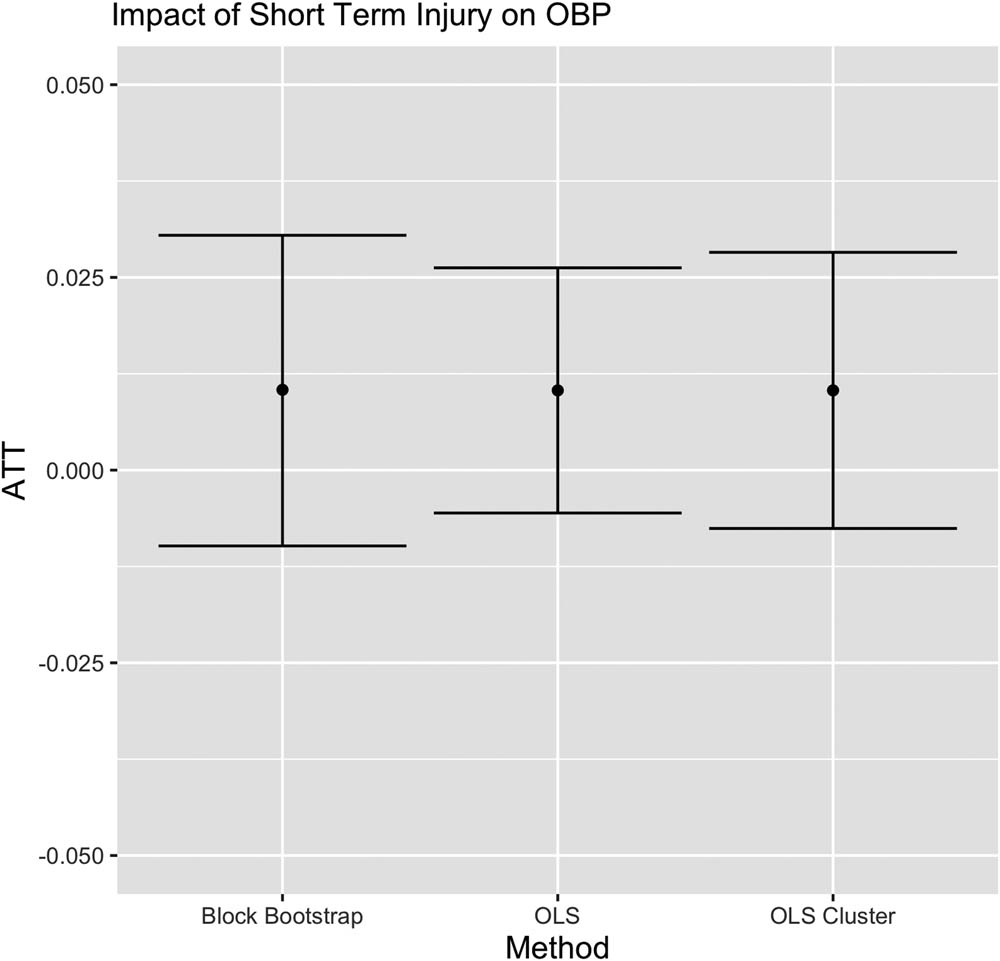
Estimates and 95% confidence intervals for block bootstrap, WLS and cluster WLS inference methods for the ATT in our 2017 baseball injury analysis.

We could have also chosen to use a difference-in-differences estimator here, using the difference in performance right before and after the injury, or pseudo-injury, date as our outcome. Results are substantively the same for both estimators. This similarity is due to the close lag OBP matches GroupMatch produces for this example.

References

[1] Stuart E. Matching methods for causal inference: a review and a look forward. Stat Sci Rev J Instit Math Stat. 2010;25:1. 10.1214/09-STS313Search in Google Scholar PubMed PubMed Central
[2] Haviland A, Nagin DS, Rosenbaum PR, Tremblay RE. Combining group-based trajectory modeling and propensity score matching for causal inferences in nonexperimental longitudinal data. Develop Psychol. 2008;44(2):422–36. 10.1037/0012-1649.44.2.422Search in Google Scholar PubMed
[3] Ben-Michael E, Feller A, Rothstein J. Synthetic controls and weighted event studies with staggered adoption. 2021. arXiv: http://arXiv.org/abs/arXiv:191203290. 10.3386/w28886Search in Google Scholar
[4] Li YP, Propert KJ, Rosenbaum PR. Balanced risk set matching. J Amer Stat Assoc. 2001;96(455):870–82. 10.1198/016214501753208573Search in Google Scholar
[5] Lu B. Propensity score matching with time-ÂŘdependent covariates. Biometrics. 2005;61:721–8. 10.1111/j.1541-0420.2005.00356.xSearch in Google Scholar PubMed
[6] Witman A, Beadles C, Liu Y, Larsen A, Kafali N, Gandhi S, et al. Comparison group selection in the presence of rolling entry for health services research: Rolling entry matching. Health Services Res. 2019;54:492–501. 10.1111/1475-6773.13086Search in Google Scholar PubMed PubMed Central
[7] Imai K, Kim IS, Wang E. Matching methods for causal inference with time-series cross-section data. Amer J Political Sci. 2020;1–19. 10.1111/ajps.12685Search in Google Scholar
[8] Acemoglu D, Naidu S, Restrepo P, Robinson JA. Democracy does cause growth. J Political Econ. 2019;127(1):47–100. 10.3386/w20004Search in Google Scholar
[9] Bohl AA, Fishman PA, Ciol MA, Williams B, LoGerfo J, Phelan EA. A longitudinal analysis of total 3-year healthcare costs for older adults who experience a fall requiring medical care. J Amer Geriatric Soc. 2010;58(5):853–60. 10.1111/j.1532-5415.2010.02816.xSearch in Google Scholar PubMed
[10] Pimentel SD, Forrow LV, Gellar J, Li J. Optimal matching approaches in health policy evaluations under rolling enrollment. J R Stat Soc Ser A (Stat Soc). 2020;183:1411–35. 10.1111/rssa.12521Search in Google Scholar
[11] Begly JP, Guss MS, Wolfson TS, Mahure SA, Rokito AS, Jazrawi LM. Performance outcomes after medial ulnar collateral ligament reconstruction in Major League Baseball positional players. J Shoulder Elbow Surgery. 2018;27:282–90. 10.1016/j.jse.2017.09.004Search in Google Scholar PubMed
[12] Conte S, Camp CL, Dines JS. Injury trends in Major League Baseball over 18 seasons: 1998–2015. Am J Orthop. 2016;45:116–23. Search in Google Scholar
[13] Frangiamore SJ, Mannava S, Briggs KK, McNamara S, Philippon MJ. Career length and performance among professional baseball players returning to play after hip arthroscopy. Amer J Sports Med. 2018;46:2588–93. 10.1177/0363546518775420Search in Google Scholar PubMed
[14] Wasserman EB, Abar B, Shah MN, Wasserman D, Bazarian JJ. Concussions are associated with decreased batting performance among major league baseball players. Amer J Sports Med. 2015;43:1127–33. 10.1177/0363546515576130Search in Google Scholar PubMed
[15] Otsu T, Rai Y. Bootstrap inference of matching estimators for average treatment effects. J Amer Statist Assoc. 2017;112:1720–32. 10.1080/01621459.2016.1231613Search in Google Scholar
[16] Athey S, Imbens GW. Design-based analysis in difference-in-differences settings with staggered adoption. J Econometric. 2022;226(1):62–79. 10.3386/w24963Search in Google Scholar
[17] Rosenbaum PR. The consequences of adjustment for a concomitant variable that has been affected by the treatment. J R Stat Soc Ser A (General). 1984;147(5):656–66. 10.2307/2981697Search in Google Scholar
[18] Hansen BB. The prognostic analogue of the propensity score. Biometrika. 2008;95(2):481–8. 10.1093/biomet/asn004Search in Google Scholar
[19] Abadie A, Imbens GW. Bias-corrected matching estimators for average treatment effects. J Business Economic Stat. 2011;29:1–11. 10.1198/jbes.2009.07333Search in Google Scholar
[20] Rubin DB. Using multivariate matched sampling and regression adjustment to control bias in observational studies. J Amer Stat Assoc. 1979:318–28. 10.1017/CBO9780511810725.013Search in Google Scholar
[21] Antonelli J, Cefalu M, Palmer N, Agniel D. Doubly robust matching estimators for high dimensional confounding adjustment. Biometrics. 2018;74(4):1171–9. 10.1111/biom.12887Search in Google Scholar PubMed PubMed Central
[22] Hansen BB. Full matching in an observational study of coaching for the SAT. J Amer Stat Assoc. 2004;99(467):609–18. 10.1198/016214504000000647Search in Google Scholar
[23] Kapelner A, Krieger A. Matching on-the-fly: sequential allocation with higher power and efficiency. Biometrics. 2014;70(2):378–88. 10.1111/biom.12148Search in Google Scholar PubMed
[24] Imbens GW. Experimental design for unit and cluster randomized trials. International Initiative for Impact Evaluation. Cuernavaca; 2011. Search in Google Scholar
[25] Abadie A, Imbens GW. Large sample properties of matching estimators for average treatment effects. Econometrica. 2006;74:235–67. 10.1111/j.1468-0262.2006.00655.xSearch in Google Scholar
[26] Abadie A, Imbens GW. On the failure of the bootstrap for matching estimators. Econometrica. 2008;76:1537–57. 10.3386/t0325Search in Google Scholar
[27] Abadie A, Imbens GW. A Martingale representation for matching estimators. J Amer Stat Assoc. 2012;107:833–43. 10.3386/w14756Search in Google Scholar
[28] Rosenbaum PR. Covariance adjustment in randomized experiments and observational studies. Stat Sci. 2002;17(3):286–327. 10.1214/ss/1042727942Search in Google Scholar
[29] Rosenbaum PR. Observational studies. New York, NY: Springer; 2002. 10.1007/978-1-4757-3692-2Search in Google Scholar
[30] Fogarty CB. Studentized sensitivity analysis for the sample average treatment effect in paired observational studies. J Amer Stat Assoc. 2020;115(531):1518–30. 10.1080/01621459.2019.1632072Search in Google Scholar
[31] Li X, Ding P. General forms of finite population central limit theorems with applications to causal inference. J Amer Stat Assoc. 2017;112(520):1759–69. 10.1080/01621459.2017.1295865Search in Google Scholar
[32] Austin PC, Small DS. The use of bootstrapping when using propensity-score matching without replacement: a simulation study. Stat Med. 2014;33(24):4306–19. 10.1002/sim.6276Search in Google Scholar PubMed PubMed Central
[33] Ho DE, Imai K, King G, Stuart EA. Matching as nonparametric preprocessing for reducing model dependence in parametric causal inference. Political Anal. 2007;15:199–236. 10.1093/pan/mpl013Search in Google Scholar
[34] Stuart EA, King G, Imai K, Ho D. MatchIt: nonparametric preprocessing for parametric causal inference. J Stat Software. 2011;42(8):1–28. 10.18637/jss.v042.i08Search in Google Scholar
[35] Abadie A, Spiess J. Robust post-matching inference. J Amer Stat Assoc. 2022;117(538):1–13.10.1080/01621459.2020.1840383Search in Google Scholar
[36] Keele L. The statistics of causal inference: A view from political methodology. Political Anal. 2015;23(3):313–35. 10.1093/pan/mpv007Search in Google Scholar
[37] Rosenbaum PR. Choice as an alternative to control in observational studies. Stat Sci. 1999;14(3):259–78. 10.1214/ss/1009212410Search in Google Scholar
[38] Hartman E, Hidalgo FD. An equivalence approach to balance and placebo tests. Amer J Political Sci. 2018;62(4):1000–13. https://onlinelibrary.wiley.com/doi/abs/10.1111/ajps.12387. 10.1111/ajps.12387Search in Google Scholar
[39] Baumer BS. Why on-base percentage is a better indicator of future performance than batting average: An algebraic proof. J Quantitat Anal Sports. 2008;4(2). https://doi.org/10.2202/1559-0410.1101. 10.2202/1559-0410.1101Search in Google Scholar
[40] Efron B, Morris C. Data analysis using Stein’s estimator and its generalizations. J Amer Stat Assoc. 1975;70:311–9. 10.1080/01621459.1975.10479864Search in Google Scholar
[41] Zhao Q, Small DS, Bhattacharya BB. Sensitivity analysis for inverse probability weighting estimators via the percentile bootstrap. J R Stat Soc Ser B (Stat Methodol). 2019;81(4):735–61. 10.1111/rssb.12327Search in Google Scholar
[42] Soriano D, Ben-Michael E, Bickel PJ, Feller A, Pimentel SD. Interpretable sensitivity analysis for balancing weights. 2021. arXiv: http://arXiv.org/abs/arXiv:210213218. Search in Google Scholar
[43] Ding P, VanderWeele TJ. Sensitivity analysis without assumptions. Epidemiology (Cambridge, Mass). 2016;27(3):368. 10.1097/EDE.0000000000000457Search in Google Scholar PubMed PubMed Central
[44] Cinelli C, Hazlett C. Making sense of sensitivity: Extending omitted variable bias. J R Stat Soc Ser B (Stat Methodol). 2020;82(1):39–67. 10.1111/rssb.12348Search in Google Scholar
[45] Rosenbaum PR, Rubin DB. Constructing a control group using multivariate matched sampling methods that incorporate the propensity score. Amer Stat. 1985;39(1):33–8. 10.1017/CBO9780511810725.019Search in Google Scholar
[46] Yu R, Silber JH, Rosenbaum PR. Matching methods for observational studies derived from large administrative databases. Stat Sci. 2020;35(3):338–55. 10.1214/19-STS699Search in Google Scholar
[47] Rosenbaum PR, Ross RN, Silber JH. Minimum distance matched sampling with fine balance in an observational study of treatment for ovarian cancer. J Amer Stat Assoc. 2007;102(477):75–83. 10.1198/016214506000001059Search in Google Scholar
[48] Zubizarreta JR. Using mixed integer programming for matching in an observational study of kidney failure after surgery. J Amer Stat Assoc. 2012;107(500):1360–71. 10.1080/01621459.2012.703874Search in Google Scholar
[49] Pimentel SD, Kelz RR, Silber JH, Rosenbaum PR. Large, sparse optimal matching with refined covariate balance in an observational study of the health outcomes produced by new surgeons. J Amer Stat Assoc. 2015;110(510):515–27. 10.1080/01621459.2014.997879Search in Google Scholar PubMed PubMed Central
© 2023 the author(s), published by De Gruyter
This work is licensed under the Creative Commons Attribution 4.0 International License.
Articles in the same Issue
- Research Articles
- Adaptive normalization for IPW estimation
- Matched design for marginal causal effect on restricted mean survival time in observational studies