2D score-based estimation of heterogeneous treatment effects

2.1 Matching

To tackle the “missing data” problem when estimating treatment effects in randomized experiments in practice, matching serves as a very powerful tool. The main goal of matching is to find matched groups with similar or balanced observed covariate distributions [20]. The exact K -nearest-neighbour matching [2] is one of the most common and easiest to implement and understand methods; ratio matching [21–23], which finds multiple good matches for each treated individual, performs well when there is a large number of control individuals. Rosenbaum [24], Gu and Rosenbaum [25], and Zubizarreta [26,27] developed various optimal matching algorithms to minimize the total sum of distances between treated units and matched controls in a global sense. Abadie and Imbens [28] studied the consistency of covariate matching estimators under large sample assumptions. Instead of greedy matching on the entire covariates, propensity score matching (PSM) by Rubin and Thomas [29] is an alternative algorithm that does not guarantee optimal balance among covariates and reduces dimension sufficiently. Imbens [30] improved propensity score matching with regression adjustment. The additional matching on prognostic factors in propensity score matching was first considered by Rubin and Thomas [22]. Later, Leacy and Stuart [6] demonstrated the superiority of the joint use of propensity and prognostic scores in matching over single score-based matching in low-dimensional settings through extensive simulation studies. Antonelli et al. [7] extended the method to fit to high-dimensional settings and derived asymptotic results for the so-called doubly robust matching estimators (DRME). The sequential works by Aikens et al. [31] and Aikens and Baiocchi [32] pioneered in visualizing the relationship between propensity and prognostic scores as auxiliary in the estimation of treatment effects.

2.2 Subclassification

To understand heterogeneity of treatment effects in the data, subclassification, first used by Cochran [33], is another important research problem. The key idea is to form subgroups over the entire population based on characteristics that are either immutable or observed before randomization. Rosenbaum and Rubin [4,34], and Lunceford and Davidian [35] examined how creating a fixed number of subclasses according to propensity scores removes the bias in the estimated treatment effects, and Yang et al. [36] developed a similar methodology in settings with more than two treatment levels. Full matching [37–39] is a more sophisticated form of subclassification that selects the number of subclasses automatically by creating a series of matched sets. Schou and Marschner [40] presented three measures derived using the theory of order statistics to claim heterogeneity of treatment effect across subgroups. Su et al. [41] pioneered in exploiting standard regression tree methods [42] in subgroup treatment effect analysis. Further, Athey and Imbens [43] derived a recursive partition of the population according to treatment effect heterogeneity. Hill [44] was the first work to advocate for the use of BART [45] for estimating heterogeneous treatment effects, followed by a significant number of research papers focusing on the seminal methodology, including Green and Kern [46], Hill and Su [47], and Hahn et al. [8]. Abadie et al. [12] introduced endogenous stratification to estimate subgroup effects for a fixed number of subgroups based on certain quantiles of the prognostic score. More recently, Padilla et al. [48] combined the fused lasso estimator with score matching methods to lead to a data-adaptive subgroup effects estimator.

2.3 Machine learning for causal inference

For the goal of analyzing treatment effect heterogeneity, supervised machine learning methods play an important role. One of the more common ways for accurate estimation with experimental and observational data is to apply regression [49] or tree-based methods [50]. From a Bayesian perspective, Heckman et al. [51] provided a principled way of adding priors to regression models, and Taddy et al. [52] developed Bayesian nonparametric approaches for both linear regression and tree models. The recent breakthrough work by Wager and Athey [9] proposed the causal forest estimator arising from random forests from Breiman [53]. More recently, Athey et al. [10] took a step forward and enhanced the previous estimator based on generalized random forests. Imai and Ratkovic [54] adapted an estimator from the support vector machine classifier with hinge loss [55]. Bloniarz et al. [56] studied treatment effect estimators with lasso regularization [57] when the number of covariates is large, and Koch et al. [58] applied group lasso for simultaneous covariate selection and robust estimation of causal effects. In the meantime, a series of papers including Qian and Murphy [59], Kü nzel et al. [60], and Syrgkanis et al. [61] focused on developing meta-learners for heterogeneous treatment effects that can take advantage of various machine learning algorithms and data structures.

2.4 Applied work

On the application side, the estimation of heterogeneous treatment effects is particularly an intriguing topic in causal inference with broad applications in scientific research. Gaines and Kuklinski [62] estimated heterogeneous treatment effects in randomized experiments in the context of political science. Dehejia and Wahba [63] explored the use of propensity score matching for nonexperimental causal studies with application in economics. Dahabreh et al. [64] investigated heterogeneous treatment effects to provide the evidence base for precision medicine and patient-centred care. Zhang et al. [65] proposed the survival causal tree method to discover patient subgroups with heterogeneous treatment effects from censored observational data. Rekkas et al. [66] examined three classes of approaches to identify heterogeneity of treatment effect within a randomized clinical trial, and Tanniou et al. [67] rendered a subgroup treatment estimate for drug trials.

4.1 Step 1

We first estimate propensity and prognostic scores for all observations in the sample. For propensity score, we apply a logistic regression on the entire covariate X and the treatment indicator Z by solving the optimization problem

where σ ( x ) = 1 1 + exp ( − x ) is the logistic function. With the coefficient vector α ˆ , we compute the estimated propensity scores e ˆ by

For prognostic score, we restrict to the controlled group and regress the outcome variable Y on the covariate X through ordinary least squares: we solve

and we estimate prognostic scores as

4.2 Step 2

Next, we perform a nearest-neighbour matching based on the two estimated scores from the previous step. We adapt the notation from Abadie and Imbens [28], and use the Mahalanobis distance norm as the distance metric in the matching algorithm. Mahalanobis distance matching, first proposed by Hansen [69], has been widely used in matching algorithms for causal inference [6,31]. It has been found to perform well when the dimension of covariates are relatively low [20], and thus, it is more suitable than using standard Euclidean distance in our case when we have only propensity scores and prognostic scores as covariates.

Formally, for the units i and j with estimated propensity scores e ˆ i , e ˆ j and propensity scores p ˆ i , p ˆ j , we define the score-based Mahalanobis distance between i and j by

where Σ denotes the variance-covariance matrix of ( e ˆ , p ˆ ) ⊤ .

Let j k ( i ) be the index j ∈ { 1 , 2 , … , n } that solves Z j = 1 − Z i and

where 1 { ⋅ } is the indicator function. This is the index of the unit that is the k th closest to unit i in terms of the distance between two scores, among the units with the treatment opposite to that of unit i . We can now construct the K -nearest-neighbour set for unit i by the set of indices for the first K matches for unit i ,

We then compute

Intuitively, the construction of Y ˜ gives a proxy of the ITE on each unit. We find K matches for each unit in the opposite treatment group based on the similarity of their propensity and prognostics scores, and the mean of the K matches is used to estimate the unobserved potential outcome for each unit.

4.3 Step 3

The last step involves denoising of the point estimates of the individual treatment effects Y ˜ obtained from Step 2. The goal is to partition all units into subgroups such that the estimated treatment effects would be constant over some 2d intervals of propensity and prognostic scores (see the left of Figure 1).

Figure 1

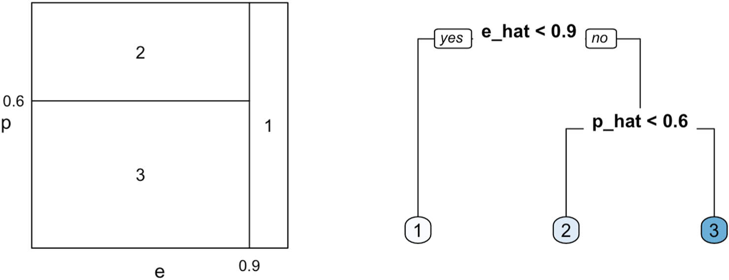
Left: a hypothetical partition over the 2d space of propensity and prognostic scores with the true values of piecewise constant treatment effects; Right: a sample regression tree T constructed in Step 3.

To perform such stratification, we grow a regression tree on Y ˜ , denoted by T , and the regressors are the estimated propensity scores e ˆ and the estimated prognostic scores p ˆ from Step 1. We follow the very general rule of binary recursive partitioning to build the tree T : allocate the data into the first two branches, using every possible binary split on every covariate; select the split that minimizes Gini impurity, and continue the optimal splits over each branch along the covariate’s values until the minimum node size is reached. To avoid overfitting, we set the minimum node size as 20 in our model. Choosing other criteria such as information gain instead of Gini impurity is another option for splitting criteria. A 10-fold cross validation is also performed at meantime to prune the large tree T for deciding the value of cost complexity. Cost complexity is the minimum improvement in the model needed at each node. The pruning rule follows that if one split does not improve the overall error of the model by the chosen cost complexity, then that split is decreed to be not worth pursuing (see more details in Section 9.2 in the study by Hastie et al. [70]).

The final tree T (see the right plot of Figure 1) contains a few terminal nodes, and these are the predicted treatment effects for all units in the data. The values exactly represent a piecewise constant stratification over the 2d space of propensity and prognostic scores.

4.4 Estimation on a new unit

After we obtain the regression tree model T in Step 3, we can now estimate the value of the individual treatment effect corresponding to a new unit with covariate x new .

We first compute the estimated propensity and prognostic scores for the new observation by

where α ˆ and θ ˆ are the solutions to equations (5) and (6), respectively. Then with the estimated propensity score e ˆ new and prognostic score p ˆ new , we can obtain an estimate of the treatment effect for this unit following the binary predictive rules in the tree T .

4.5 High-dimensional estimator

In a high-dimensional setting where the covariate dimension d is much larger than the sample size n , we can estimate the propensity and prognostic scores by adding a lasso ( l 1 -based) penalty [57] instead. This strategy was first proposed and named as DRME by Antonelli et al. [7]. The corresponding optimization problems for the two scores can be written as follows:

The selection of the tuning parameters λ 1 and λ 2 can be determined by any information criteria (AIC, BIC, etc.). In practice, we use 10-fold cross-validation (CV) to select the value of λ . Then we perform the K -nearest-neighbour matching based on propensity and prognostic scores to obtain the estimates of individual treatment effects using equation (7).

We extend the aforementioned estimator with our proposal of applying a regression tree on the estimated propensity and prognostic scores. The procedure for estimation of subgroup heterogeneous treatment effects and estimation on a new unit remains the same as Step 3 for low-dimensional setups.

4.6 Computational complexity

Our method is composed of three steps as introduced before. We first need to implement a logistic regression for estimating propensity score for a sample with size n and ambient dimension d . To solve a logistic regression optimization problem involves using the proximal Newton method, and its computational complexity is of # of iterations ⋅ O ( n d ) [74]. In general, the algorithm converges after a small number of iterations, and we can safely assume it is of a constant order. As a result, the overall time complexity of solving a logistic regression is O ( n d ) . The estimation of prognostic scores also requires a computational cost of O ( n d ) , and for high-dimensional settings, the cost of solving the solution via coordinate descent remains at O ( n d ) [75]. The complexity of a K -nearest-neighbour matching based on the two estimated scores in the second step is of O ( K n ) [76], and the selection of K ≈ log ( n ) leads to a complexity of O ( n log n ) . In the third step, we grow a regression tree based on two estimated scores, and it requires a computational complexity of O ( n log n ) .

The overall computational complexity of our method depends on the comparison between the order of d and log ( n ) . Our method attains a computational complexity of O ( n d ) if the order of d is greater than that of log ( n ) . Otherwise, the complexity becomes O ( n log n ) .

5.1 Simulated data

We first examine on the following simulated data sets under six different data generation mechanisms. We obtain insights from the simulation study by Leacy and Stuart [6] for the models considered in Scenarios 1–3. The propensity score and outcome (prognosis) models in Scenarios 1 and 3 are characterized by additivity and linearity (main effects only), but with different piecewise constant structures in the true treatment effects over a 2d grid of the two scores. We add nonadditivity and nonlinear terms to both propensity and prognosis models in Scenarios 2. In other words, both propensity and prognostic scores are expected to be misspecified in these two models if we apply generalized linear models directly in estimation. Scenario 4 comes from Abadie et al. [12], with a constant treatment effect over all observations. Scenario 5 is modified from the study by Wager and Athey [9] (see Equation 27 there), in which the propensity model follows a continuous distribution instead of a linear structure. In addition, the true treatment effect is not a function of propensity and prognostic scores. In Scenario 6, we break the mold assumption of nicely delineated subgroups in treatment effects over 2d space of the two scores, and use a smooth function instead. A high-dimensional setting ( d ≫ n ) is examined in Scenario 7, where the generative model inherits from Scenario 1. We also include a table summarizing all simulation scenarios in Appendix B to help the audience interpret the result of the simulation study more readily.

We first introduce some notations used in the experiments: the sample size n , the ambient dimension d , as well as the following functions:

Throughout all the models we consider, we maintain the unconfoundedness assumption discussed in Section 3, generate the covariate X following a certain distribution, and entail homoscedastic Gaussian noise ε .

We evaluate the accuracy of an estimator τ ( X ) by the mean-squared error for estimating τ * ( X ) at a random example X , with m = n ∕ 10 , defined by

We record the averaged mean squared error (MSE) over 1,000 Monte Carlo trials for each scenario. For each Monte Carlo trial, we use train-test split to evaluate model performance. In detail, we first obtain n training sample and train models on this set. We then generate a separate testing sample under the same data generation mechanism with sample size n ∕ 10 . We make predictions on the test data using the trained models and compute the MSEs from different models accordingly. In terms of uncertainty quantification, we measure the coverage probability of τ ( X ) with a target coverage rate of 0.95. For endogenous stratification and our proposed method, we use nonparametric bootstrap with replacement to construct the empirical quantiles for each unit. The details on the implementation of nonparametric bootstrap methods are presented in Appendix C. For causal forest, we construct 95% confidence intervals by estimating the standard errors of estimation using the “grf” package. We do not include the results for Scenario 7, a high-dimensional setting, because the asymptotic normality guarantees of nonparametric bootstrap and random forests are not valid in high dimensions [9,79].

Scenario 1. With d ∈ { 2 , 10 , 50 } , n ∈ { 1,000 , 5,000 } , for i = 1 , … , n , we generate the data as follows:

where β e and β p are randomly generated from U [ − 1 , 1 ] d in each iteration.

Scenario 2. We now add some interaction and nonlinear terms to the propensity and prognostic models in Scenario 1, while keeping the setups of the covariate X , the response Y , the true treatment effect τ * , and the error term ε unchanged. We set d = 10 and n = 5,000 in this case.

Again for each simulation, β e and β p are randomly generated from U [ − 1 , 1 ] d .

Scenario 3. In this case, we define the true treatment effect with a more complicated piecewise constant structure over the 2d grid, under the same model used in Scenario 1, with d = 10 and n = 5,000 :

Scenario 4. Setting d = 10 and n = 5,000 , the data are generated as follows:

where β = ( 1 , … , 1 ) ⊤ ∈ R d . Moreover, the treatment indicators for the simulations are such that ∑ i Z i = ⌈ n ∕ 2 ⌉ . By construction, the vector of treatment effects satisfies τ * = 0 .

Scenario 5. The data satisfy

where e 1 = ( 1 , 0 , … , 0 ) ⊤ . We compare the results of different methods under the setting: d = 10 , n = 5,000 .

Scenario 6. For this scenario, we examine the performance when the treatment effect takes on a smooth interval of propensity and prognostic scores. We use the same model in Scenario 1 for generating the two scores with d = 10 and n = 5,000 , and we inherit and modify the generative function (28) from the study by Wager and Athey [9] for treatment effects as follows:

Scenario 7. In the last case, we study the performance of different estimators on a high-dimensional data. The data model follows

We select n = 3,000 and d = 5,000 for analysis.

The boxplots that depict the distribution of MSEs obtained under all scenarios are presented in Figure 2. We can see that for Scenario 1, our proposed estimator achieves better accuracy when the sample size n is large, and it is the best among the three estimators in these cases. The good performance of our method is consistent when we assume a more complex partition on the defined 2d grid as in Scenario 3. In addition, variation in accuracy, measured by the difference between the upper quartiles and the lower quartiles (also referred as the interquartile ranges) in each boxplot becomes smaller, accompanied with the increase in n . The reason for the enhanced performance when applying our method on a large-size data is the nature of nearest neighbour algorithm, which benefits more in learning the boundaries of clusters accurately with a larger sample size. Moreover, causal random forest suffers more in accuracy especially as d gets larger [9], while our method does not impact significantly because it focuses on a low-dimensional space of the two scores instead of the overall covariate space. In Scenario 2, we introduce nonadditivity and nonlinear terms into the data model. Although linear assumptions are violated for both propensity and prognostic models, our method performs better compared to the other two methods regarding accuracy and variability. For a potential outcome model with randomized assignment of treatment and constant treatment effects, as in Scenario 4, our method has the best accuracy among all candidates, even though large noise is added to the true signal. In Scenario 5, our estimator performs slightly worse than causal forests in accuracy since the true treatment function is not directly dependent on propensity and prognostic scores, but it still outperforms endogenous stratification. However, for the previous two cases, our method shows larger variation in accuracy than the others. One of the reasons for this phenomenon is due to the misspecification in estimating the true scores and the large variance in constructing tree models. When the assumption of a sharp stratification of treatment effects in the 2d space of the two scores is invalid, as shown in Scenario 6, our method maintains its superiority over the benchmarks. With subgroups identified over the 2d interval of the scores, the mean squared errors are reduced through our estimator comparably better than the other methods. In a high-dimensional setting such as Scenario 7, we consider modified methods with lasso-regularized regressions for both our methodology and endogenous stratification, and our method remains its high performance as in the low-dimensional setups since the piecewise constant structure in treatment effects in the setting does not change.

Figure 2

Comparison of mean squared errors over 1,000 Monte Carlo simulations under different generative models for our proposed method (PP), endogenous stratification (ST), and causal forest (CF).

We now take a careful look at the visualization comparison between the true treatment effect and the predictions obtained from our method for Scenarios 1, 2, 3, 6, and 7. We confine both the true signal and the predictive model in a 2d grid scaled on the true propensity and prognostic scores, as shown in Figure 3. It is not surprising that our proposed estimators provide a descent recovery of the piecewise constant partition in the true treatment effects over the 2d grid as in Scenarios 1, 2, 3, and 7, with only a small difference in the magnitude of treatment effects. In the setting when treatment effects are smoothly distributed across the grid of the two scores as in Scenario 6, our estimation does not exactly capture the soft boundary of the shape, but still provides us with a simplified delineation that help us understand general heterogeneity in treatment effects over the 2d space.

Figure 3

One instance comparison between the true treatment effects and the estimates from the score-based method for Scenarios 1, 2, 3, 6, and 7 (from the top to the bottom). Plots on the left column depict the true treatment effect on the 2d grid of propensity and prognostic scores, and the right plots demonstrate the estimated treatment effects from our proposed method over the same grid.

With regard to uncertainty quantification, we examine coverage rates with a target confidence level of 0.95 for each method under different scenarios, and the corresponding results, along with the within iteration standard error estimates, are recorded in Table 1. It is quite clear that our proposed method achieves nominal coverage over the other two methods in almost all scenarios. It is worth to notice that although our estimator achieves a better coverage rate than the benchmarks, it suffers from large variation due to the nature of nearest-neighbour matching, especially in the case with small sample size. In general, our method that incorporates both propensity and prognostic scores in identifying subgroups and estimating treatment effects show its advantage in reducing bias, but the resulting large variance is worrisome and it remains space for future study to solve this issue.

We also compare the computational cost of our proposed scored-based method and causal forest, with simulated data from Scenario 1. Endogenous stratification is not considered in this comparison because the method exerts an arbitrary subclassification into a predetermined number of subgroups, and it does not involve a cross-validation process. We record the averaged time consumed to obtain the estimate over 1,000 simulations for both methods. Figure 4 demonstrates that our proposed method (PP) is comparably time-efficient over its competitor, and CF can be very expensive in operational time for large-size problems.

Figure 4

A plot of time per simulation in seconds for our proposed method (PP) and CF against problem size n (50 values from 1,000 up to 10,000). For each method, the time to compute the estimate for one simulated data is averaged over 1,000 Monte Carlo simulations.

These results highlight the promise of our method for accurate estimation of subgroups in heterogeneous treatment effects, all while emphasizing avenues for further work. An immediate challenge is to control the bias in estimation of propensity and prognostic scores. Using more powerful models instead of simple linear regression in estimation is a good way to reduce bias by enabling the trees to focus more closely on the coordinates with the greatest signal. The study of splitting rules for trees designed to estimate causal effects is still in its infancy and improvements may be possible.

5.2 Real data analysis

To illustrate the behaviour of our estimator, we apply our method on the two real-world data sets, one from a clinical study and the other from a complex social survey. Propensity score-based methods are frequently used for confounding adjustment in observational studies, where baseline characteristics can affect the outcome of policy interventions. Therefore, the results from our method are expected to provide meaningful implications for these real data sets. However, one potential limitation of our proposed tree-based approach is that it imposes arbitrary dichotomization with sharp thresholds and thus may obscure potential continuous gradient over the space. For real data analysis in general, our method provides a reasonable simplification that is easy to interpret for the audience and gives some framework for thinking about when such a simplification would be appropriate.

5.2.1 Right heart catheterization (RHC) analysis

While randomized control trials are widely encouraged as the ideal methodology for causal inference in clinical and medical research, the lack of randomized data due to high costs and potential high risks leads to the studies based on observational data. In this section, we are interested in examining the association between the use of RHC during the first 24 h of care in the intensive care unit (ICU) and the short-term survival conditions of the patients. RHC is a procedure for directly measuring how well the heart is pumping blood to the lungs. RHC is often applied to critically ill patients for directing immediate and subsequent treatment. However, RHC imposes a small risk of causing serious complications when administering the procedure. Therefore, the use of RHC is controversial among practitioners, and scientists want to statistically validate the causal effects of RHC treatments. The causal study using observational data can be dated back to Connors et al. [80], where the authors implemented propensity score matching and concluded that RHC treatment lead to lower survival than not performing the treatment. Later, Hirano and Imbens [81] proposed a more efficient propensity-score-based method, and the recent study by Loh and Vansteelandt [82] using a modified propensity score model suggested that RHC significantly affected mortality rate in a short-term period.

A dataset for analysis was first used in the study by Connors et al. [80], and it is suitable for the purpose of applying our method because of its extremely well-balanced distribution of confounders across levels of the treatment [83]. The treatment variable Z in the data indicates whether a patient received a RHC within 24 hours of admission. The binary outcome Y is defined based on whether a patient died at any time up to 180 days since admission. The original data consisted of 5,735 participants with 73 covariates. We preprocess the full data in the way suggested in the Hirano and Imbens [81] and Loh and Vansteelandt [82], by removing all observations that contain null values in covariates, dropping the singular covariate in the reduced data, and encoding categorical variables into dummy variables. The resulted data contains 2,707 observations and 72 covariates, with 1,103 in the treated group ( Z = 1 ) and 1,604 in the control group ( Z = 0 ). Among the 72 observed covariates, there are 21 continuous, 25 binary, and 26 dummy variables transformed from the original six categorical variables.

The result of the prediction model from our proposed method is reported in Figure 5. We observe that the sign of estimated treatment effects varies depending on the value of the propensity score and prognostic score. This particular pattern implies that RHC procedures indeed offer both benefits and risks in affecting patients’ short-term survival conditions. Specifically, we are interested in the occurrence of large positive treatment effects (increase in chance of death) from the estimation. An estimated treatment effect of 0.17 (with a 95% confidence interval between − 0.25 and 1.00) is observed on the group of patients with propensity scores less than 0.64 and prognostic scores less than 0.74, and this group accounts for 56% of the entire sample. For the rest of the sample, we observe relatively small treatment effects in magnitude. Under the scenario of RHC data, a smaller propensity score means that the patient is less likely to receive RHC procedures after admitting to the ICU, and it is related to the availability of RHC procedures at the hospital to which the patient is admitted. A smaller prognostic score tells that the patient has lower underlying chance of death. One possible explanation for this significant positive treatment on this certain group is that drastic change in treatment procedures that were applied to patients who do not actually need the aggressive style of care largely undermine patients’ health conditions after admission and increase the mortality rate. In summary, our findings generally agree with the results and explanations presented in the study by Connors et al. [80], and they offer some insights for practitioners to decide whether they should apply RHC procedures to patients.

Figure 5

Prediction model for RHC data. Left: a tree diagram of predictions on each split based on the two scores, with 95% confidence intervals provided on the bottom. Right: a 2d plot of prediction stratification on the intervals of propensity and prognostic scores, with a colour scale on magnitude of treatment effects.

5.2.2 National medical expenditure survey (NMES)

For the next experiment, we analyze a complex social survey data. In many complex surveys, data are not usually well balanced due to potential biased sampling procedure. To incorporate score-based methods with complex survey data requires an appropriate estimation on propensity and prognostic scores. DuGoff et al. [84] suggested that combining a propensity score method and survey weighting is necessary to achieve unbiased treatment effect estimates that are generalizable to the original survey target population. Austin et al. [85] conducted numerical experiments and showed that greater balance in measured baseline covariates and decreased bias is observed when natural retained weights are used in propensity score matching. Therefore, we include sampling weight as an baseline covariate when estimating propensity and prognostic scores in our analysis.

In this study, we aim to answer the research question: how smoking habit affects medical expenditure over lifetime, and we use the same data set as given in the study by Johnson et al. [86], which is originally extracted from the 1987 NMES. The NMES included detailed information about frequency and duration of smoking with a large nationally representative data base of nearly 30,000 adults, and that 1987 medical costs are verified by multiple interviews and additional data from clinicians and hospitals. A large amount of literature focus on applying various statistical methods to analyze the causal effects of smoking on medical expenditures using the NMES data. In the original study by Johnson et al. [86], the authors first estimated the effects of smoking on certain diseases and then examined how much those diseases increased medical costs. In contrast, Rubin [87], Imai and van Dyk [88], and Zhao et al. [89] proposed to directly estimate the effects of smoking on medical expenditures using propensity-score-based matching and subclassification. Hahn et al. [8] applied Bayesian regression tree models to assess heterogeneous treatment effects.

For our analysis, we explore the effects of extensive exposure to cigarettes on medical expenditures, and we use pack-year as a measurement of cigarette measurement, the same as given in the studies by Imai and van Dyk [88] and Hahn et al. [8]. Pack-year is a clinical quantification of cigarette smoking used to measure a person’s exposure to tobacco, defined by

Pack-year = Number of cigarettes per day 20 × Number of years smoked .

Following that, we determine the treatment indicator Z by the question whether the observation has a heavy lifetime smoking habit, which we define to be greater than 17 pack-years, the equivalent of 17 years of pack-a-day smoking.

The subject-level covariates X in our analysis include age at the times of the survey (between 19 and 94), age when the individual started smoking, gender (male, female), race (white, black, other), marriage status (married, widowed, divorced, separated, never married), education level (college graduate, some college, high school graduate, other), census region (Northeast, Midwest, South, West), poverty status (poor, near poor, low income, middle income, high income), seat belt usage (rarely, sometimes, always/almost always), and sample weight. We select the natural logarithm of annual medical expenditures as the outcome variable Y to maintain the assumption of heteroscedasticity in random errors. We preprocess the raw data set by omitting any observations with missing values in the covariates and excluding those who had zero medical expenditure. The resulting restricted data set contains 7,903 individuals, with 4,014 in the treated group ( Z = 1 ) and 3,889 in the controlled group ( Z = 0 ).

The prediction model obtained from our method, as shown in Figure 6, is simple and easy to interpret. We derive a positive treatment effect across the entire sample, and the effect becomes significant when the predicted potential outcome is relatively low (less than 5.7). These results indicate that more reliance on smoking will deteriorate one’s health condition, especially for those who currently do not have a large amount of medical expenditure. Moreover, we observe a significant positive treatment effect of 1.4 (with a 95% confidence interval between 0.56 and 2.79), and in other words, a certain and substantial increase in medical expenditure for the subgroup with propensity score less than 0.17. It is intuitive to assume that a smaller possibility of engaging in excessive tobacco exposure is associated with healthier living styles. This phenomenon is another evidence that individuals who are more likely to stay healthy may suffer more from excessive exposure to tobacco products. In all, these results support policymakers and social activists who advocate for nationwide smoking ban.

Figure 6

Prediction model for NMES data. Left: a tree diagram of predictions on each split based on the two scores, with 95% confidence intervals provided on the bottom. Right: a 2d plot of prediction stratification on the intervals of propensity and prognostic scores, with a colour scale on magnitude of treatment effects.

References

[1] Neyman J. On the application of probability theory to agricultural experiments. Ann Agricult Sci. 1923;10:1–51. Search in Google Scholar
[2] Rubin DB. Estimating causal effects of treatments in randomized and nonrandomized studies. J Educ Psychol. 1974;66(5):688–701. 10.1037/h0037350Search in Google Scholar
[3] Hahn J. On the role of the propensity score in efficient semiparametric estimation of average treatment effects. Econometrica. 1998;66(2):315–31. 10.2307/2998560Search in Google Scholar
[4] Rosenbaum PR, Rubin DB. The central role of the propensity score in observational studies for causal effects. Biometrika. 1983;70(1):41–55. 10.1093/biomet/70.1.41Search in Google Scholar
[5] Hansen BB. The prognostic analogue of the propensity score. Biometrika. 2008;95(2):481–8. 10.1093/biomet/asn004Search in Google Scholar
[6] Leacy FP, Stuart EA. On the joint use of propensity and prognostic scores in estimation of the average treatment effect on the treated: a simulation study. Stat Med. 2014;33(20):3488–508. 10.1002/sim.6030Search in Google Scholar PubMed PubMed Central
[7] Antonelli J, Cefalu M, Palmer N, Agniel D. Doubly robust matching estimators for high dimensional confounding adjustment. Biometrics. 2018;74(4):1171–9. 10.1111/biom.12887Search in Google Scholar PubMed PubMed Central
[8] Hahn PR, Murray JS, Carvalho CM. Bayesian regression tree models for causal inference: regularization, confounding, and heterogeneous effects. Bayesian Anal. 2020;15(3):965–1056. 10.1214/19-BA1195Search in Google Scholar
[9] Wager S, Athey S. Estimation and inference of heterogeneous treatment effects using random forests. J Amer Stat Assoc. 2018;113(523):1228–42. 10.1080/01621459.2017.1319839Search in Google Scholar
[10] Athey S, Tibshirani J, Wager S. Generalized random forests. Ann Stat. 2019;47(2):1148–78. 10.1214/18-AOS1709Search in Google Scholar
[11] Assmann SF, Pocock SJ, Enos LE, Kasten LE. Subgroup analysis and other (mis)uses of baseline data in clinical trials. Lancet. 2000;355(9209):1064–9. 10.1016/S0140-6736(00)02039-0Search in Google Scholar PubMed
[12] Abadie A, Chingos MM, West MR. Endogenous stratification in randomized experiments. Rev Econ Stat. 2018;C(4):567–80. 10.1162/rest_a_00732Search in Google Scholar
[13] Kent DM, Hayward RA. Limitations of applying summary results of clinical trials to individual patients: the need for risk stratification. J Amer Med Assoc. 2007;298(10):1209–12. 10.1001/jama.298.10.1209Search in Google Scholar PubMed
[14] Keele L. The statistics of causal inference: a view from political methodology. Political Anal. 2015;23(3):313–35. 10.1093/pan/mpv007Search in Google Scholar
[15] Ding P, Li F. Causal inference: a missing data perspective. Stat Sci 2018;33(2):214–37. 10.1214/18-STS645Search in Google Scholar
[16] Holland PW. Statistics and causal Inference. J Amer Stat Assoc. 1986;81(396):945–60. 10.1080/01621459.1986.10478354Search in Google Scholar
[17] Dawid AP. Causal inference without counterfactuals. J Amer Stat Assoc. 2000;95(450):407–24. 10.1080/01621459.2000.10474210Search in Google Scholar
[18] Pearl J. Causal diagrams for empirical research. Biometrika 1995;82(4):669–710. 10.1093/biomet/82.4.702Search in Google Scholar
[19] Pearl J. Causality: models, reasoning, and inference. Cambridge, UK: Cambridge University Press; 2009. 10.1017/CBO9780511803161Search in Google Scholar
[20] Stuart EA. Matching methods for causal inference: a review and a look forward. Stat Sci Rev J Inst Math Stat. 2010;25(1):1–21. 10.1214/09-STS313Search in Google Scholar PubMed PubMed Central
[21] Smith H. Matching with multiple controls to estimate treatment effects in observational studies. Sociol Methodol. 1997;27(1):325–53. 10.1111/1467-9531.271030Search in Google Scholar
[22] Rubin DB, Thomas N. Combining propensity score matching with additional adjustments for prognostic covariates. J Amer Stat Assoc. 2000;95(450):573–85. 10.1080/01621459.2000.10474233Search in Google Scholar
[23] Ming K, Rosenbaum PR. A note on optimal matching with variable controls using the assignment algorithm. J Comput Graph Stat. 2001;10(3):455–63. 10.1198/106186001317114938Search in Google Scholar
[24] Rosenbaum PR. Optimal matching for observational studies. J Amer Stat Assoc.1989;84(408):1024–32. 10.1080/01621459.1989.10478868Search in Google Scholar
[25] Gu XS, Rosenbaum PR. Comparison of multivariate matching methods: structures, distances, and algorithms. J Comput Graph Stat. 1993;2(4):405–20. 10.1080/10618600.1993.10474623Search in Google Scholar
[26] Zubizarreta JR. Using mixed integer programming for matching in an observational study of kidney failure after surgery. J Amer Stat Assoc. 2012107(500):1360–71. 10.1080/01621459.2012.703874Search in Google Scholar
[27] Zubizarreta JR, Keele L. Optimal multilevel matching in clustered observational studies: a case study of the effectiveness of private schools under a large-scale voucher system. J Amer Stat Assoc. 2017;112(518):547–60. 10.1080/01621459.2016.1240683Search in Google Scholar
[28] Abadie A, Imbens GW. Large sample properties of matching estimators for average treatment effects. Econometrica. 2006;74(1):235–67. 10.1111/j.1468-0262.2006.00655.xSearch in Google Scholar
[29] Rubin DB, Thomas N. Matching using estimated propensity scores: relating theory to practice. Biometrics. 1996;52(1):249–64. 10.2307/2533160Search in Google Scholar
[30] Imbens GW. Nonparametric estimation of average treatment effects under exogeneity: a review. Rev Econ Stat. 2004;86:4–29. 10.1162/003465304323023651Search in Google Scholar
[31] Aikens RC, Greaves D, Baiocchi M. A pilot design for observational studies: using abundant data thoughtfully. Stat Med. 2020;39(30):4821–40. 10.1002/sim.8754Search in Google Scholar PubMed
[32] Aikens RC, Baiocchi M. Assignment-control plots: a visual companion for causal inference study design. Amer Stat. 2023;77(1):72–84. 10.1080/00031305.2022.2051605Search in Google Scholar PubMed PubMed Central
[33] Cochran WG. The effectiveness of adjustment by subclassification in removing bias in observational studies. Biometrics. 1968;24(2):295–313. 10.2307/2528036Search in Google Scholar
[34] Rosenbaum PR, Rubin DB. Constructing a control group using multivariate matched sampling methods that incorporate the propensity score. Amer Stat. 1985;39(1):33–38. 10.1080/00031305.1985.10479383Search in Google Scholar
[35] Lunceford JK, Davidian M. Stratification and weighting via the propensity score in estimation of causal treatment effects: a comparative study. Stat Med. 2004;23(19):2937–60. 10.1002/sim.1903Search in Google Scholar PubMed
[36] Yang S, Imbens GW, Cui Z, Faries DE, Kadziola Z. Propensity score matching and subclassification in observational studies with multi-level treatments. Biometrics. 2016;72(4):1055–65. 10.1111/biom.12505Search in Google Scholar PubMed
[37] Rosenbaum PR. A characterization of optimal designs for observational studies. J R Stat Soc Ser B (Stat Methodol). 1991;53(3):597–610. 10.1111/j.2517-6161.1991.tb01848.xSearch in Google Scholar
[38] Hansen BB. Full matching in an observational study of coaching for the SAT. J Amer Stat Assoc. 2004;99(467):609–18. 10.1198/016214504000000647Search in Google Scholar
[39] Stuart EA, Green KM. Using full matching to estimate causal effects in non-experimental studies: examining the relationship between adolescent marijuana use and adult outcomes. Development Psychol. 2008;44(2):395–406. 10.1037/0012-1649.44.2.395Search in Google Scholar PubMed PubMed Central
[40] Schou IM, Marschner IC. Methods for exploring treatment effect heterogeneity in subgroup analysis: an application to global clinical trials. Pharmaceut Stat. 2015;14(1):44–55. 10.1002/pst.1656Search in Google Scholar PubMed
[41] Su X, Tsai C, Wang H, Nickerson DM, Li B. Subgroup analysis via recursive partitioning. J Machine Learn Res. 2009;10:141–58. 10.2139/ssrn.1341380Search in Google Scholar
[42] Breiman L, Friedman J, Stone CJ, Olshen RA. Classification and regression trees. New York: Taylor & Francis; 1984. Search in Google Scholar
[43] Athey S, Imbens GW. Recursive partitioning for heterogeneous causal effects. Proc Nat Acad Sci. 2016;113(27):7353–60. 10.1073/pnas.1510489113Search in Google Scholar PubMed PubMed Central
[44] Hill JL. Bayesian nonparametric modeling for causal inference. J Comput Graph Stat. 2011;20(1):217–40. 10.1198/jcgs.2010.08162Search in Google Scholar
[45] Chipman HA, George EI, McCulloch RE. BART: Bayesian additive regression trees. Ann Appl Stat. 2010;4(1):266–98. 10.1214/09-AOAS285Search in Google Scholar
[46] Green DP, Kern HL. Modeling heterogeneous treatment effects in survey experiments with Bayesian additive regression trees. Public Opinion Quarter. 2012;76(3):491–511. 10.1093/poq/nfs036Search in Google Scholar
[47] Hill JL, Su Y. Assessing lack of common support in causal inference using Bayesian nonparametrics: implications for evaluating the effect of breastfeeding on childrenas cognitive outcomes. Ann Appl Stat. 2013;7(3):1386–420. 10.1214/13-AOAS630Search in Google Scholar
[48] Padilla OHM, Ding P, Chen Y, Ruiz G. A causal fused lasso for interpretable heterogeneous treatment effects estimation. 2021. arXiv: 2110.00901. Search in Google Scholar
[49] Imbens GW, Rubin DB. Causal inference for statistics, social, and biomedical sciences: an introduction. Cambridge, UK: Cambridge University Press; 2015. 10.1017/CBO9781139025751Search in Google Scholar
[50] Imai K, Strauss A. Estimation of heterogeneous treatment effects from randomized experiments, with application to the optimal planning of the get-out-the-vote campaign. Politic Anal. 2011;19:1–19. 10.1093/pan/mpq035Search in Google Scholar
[51] Heckman JJ, Lopes HF, Piatek R. Treatment effects: a Bayesian perspective. Econom Rev. 2014;33(1–4):36–67. 10.1080/07474938.2013.807103Search in Google Scholar PubMed PubMed Central
[52] Taddy M, Gardner M, Chen L, Draper D. A nonparametric Bayesian analysis of heterogenous treatment effects in digital experimentation. J Business Econom Stat. 2016;34(4):661–72. 10.1080/07350015.2016.1172013Search in Google Scholar
[53] Breiman L. Random forests. Machine Learning. 2001;45:5–32. 10.1023/A:1010933404324Search in Google Scholar
[54] Imai K, Ratkovic M. Estimating treatment effect heterogeneity in randomized program evaluation. Ann Appl Stat. 2013;7(1):443–70. 10.1214/12-AOAS593Search in Google Scholar
[55] Wahba G. Soft and hard classification by reproducing kernel Hilbert space methods. Proc Nat Acad Sci. 2002;99(26):16524–30. 10.1073/pnas.242574899Search in Google Scholar PubMed PubMed Central
[56] Bloniarz A, Liu H, Zhang C, Sekhon JS, Yu B. Lasso adjustments of treatment effect estimates in randomized experiments. Proc Nat Acad Sci. 2016;113(27):7383–90. 10.1073/pnas.1510506113Search in Google Scholar PubMed PubMed Central
[57] Tibshirani R. Regression shrinkage and selection via the lasso. J R Stat Soc Ser B (Stat Meth) 1996;58(1):267–88. 10.1111/j.2517-6161.1996.tb02080.xSearch in Google Scholar
[58] Koch B, Vock DM, Wolfson J. Covariate selection with group lasso and doubly robust estimation of causal effects. Biometrics. 2018;74(1):8–17. 10.1111/biom.12736Search in Google Scholar PubMed PubMed Central
[59] Qian M, Murphy SA. Performance guarantees for individualized treatment rules. Ann Stat 2011;39(2):1180–210. 10.1214/10-AOS864Search in Google Scholar PubMed PubMed Central
[60] Kü nzel SR, Sekhon JS, Bickel PJ, Yu B. Metalearners for estimating heterogeneous treatment effects using machine learning. Proc Nat Acad Sci. 2019;116(10):4156–65. 10.1073/pnas.1804597116Search in Google Scholar PubMed PubMed Central
[61] Syrgkanis V, Lei V, Oprescu M, Hei M, Oprescu M, Battocchi K, et al. Machine learning estimation of heterogeneous treatment effects with instruments. Advances in Neural Information Processing Systems 32: Annual Conference on Neural Information Processing Systems 2019, NeurIPS 2019, December 8-14, 2019, Vancouver, BC, Canada. p. 15167–76. Search in Google Scholar
[62] Gaines B, Kuklinski J. Estimation of heterogeneous treatment effects related to self-selection. Amer J Politic Sci. 2011;55(3):724–36. 10.1111/j.1540-5907.2011.00518.xSearch in Google Scholar
[63] Dehejia RH, Wahba S. Propensity score matching methods for nonexperimental causal studies. Rev Econ Stat. 2002;84(1):151–61. 10.1162/003465302317331982Search in Google Scholar
[64] Dahabreh IJ, Hayward R, Kent DM. Using group data to treat individuals: understanding heterogeneous treatment effects in the age of precision medicine and patient-centred evidence. Int J Epidemiol. 2016;45(6):2184–93. 10.1093/ije/dyw125Search in Google Scholar PubMed PubMed Central
[65] Zhang W, Le TD, Liu L, Zhou Z, Li J. Mining heterogeneous causal effects for personalized cancer treatment. Bioinformatics. 2017;33(15):2372–8. 10.1093/bioinformatics/btx174Search in Google Scholar PubMed
[66] Rekkas A, Paulus JK, Raman G, Wong JB, Steyerberg EW, Rijnbeek PR, et al. Predictive approaches to heterogeneous treatment effects: a scoping review. BMC Med Res Methodol. 2020;20(1):264. 10.1186/s12874-020-01145-1Search in Google Scholar PubMed PubMed Central
[67] Tanniou J, van der Tweel I, Teerenstra S, Roes KCB. Estimates of subgroup treatment effects in overall nonsignificant trials: to what extent should we believe in them? Pharmaceut Stat. 2017;16(4):280–95. 10.1002/pst.1810Search in Google Scholar PubMed
[68] D’Amour A, Ding P, Feller A, Lei L, Sekhon J. Overlap in observational studies with high-dimensional covariates. J Econ. 2021;221:644–54. 10.1016/j.jeconom.2019.10.014Search in Google Scholar
[69] Hansen BB. Bias reduction in observational studies via prognosis scores. Statistics Department, University of Michigan; Ann Arbor, Michigan: Technical Report. 2006. 441. Search in Google Scholar
[70] Hastie T, Tibshirani R, Friedman J. The elements of statistical learning: data mining, inference, and prediction. New York: Springer; 2001. 10.1007/978-0-387-21606-5Search in Google Scholar
[71] Austin PC, Schuster T. The performance of different propensity score methods for estimating absolute effects of treatments on survival outcomes: a simulation study. Stat Meth Med Res. 2016;25(5):2214–37. 10.1177/0962280213519716Search in Google Scholar PubMed PubMed Central
[72] Ming K, Rosenbaum PR. Substantial gains in bias reduction from matching with a variable number of controls. Biometrics. 2001;56(1):118–24. 10.1111/j.0006-341X.2000.00118.xSearch in Google Scholar
[73] Brito MR, Chávez EL, Quiroz AJ, Yukich JE. Connectivity of the mutual k-nearest-neighbour graph in clustering and outlier detection. Stat Probability Lett. 1997;35(1):33–42. 10.1016/S0167-7152(96)00213-1Search in Google Scholar
[74] Yuan G, Ho C, Lin C. An improved GLMNET for l1-regularized logistic regression. J Machine Learn Res. 2012;13:1999–2030. 10.1145/2020408.2020421Search in Google Scholar
[75] Friedman J, Hastie T, Tibshirani R. Regularization paths for generalized linear models via coordinate descent. J Stat Softw. 2010;33(1):1–22. 10.18637/jss.v033.i01Search in Google Scholar
[76] von Luxburg U. A tutorial on spectral clustering. Stat Comput. 2007;17(4):395–416. 10.1007/s11222-007-9033-zSearch in Google Scholar
[77] Athey S, Wager S. Estimating treatment effects with causal forests: an application. Observ Stud. 2019;19(5):37–51. 10.1353/obs.2019.0001Search in Google Scholar
[78] Nie X, Wager S. Quasi-oracle estimation of heterogeneous treatment effects. Biometrika. 2021;108(2):299–319. 10.1093/biomet/asaa076Search in Google Scholar
[79] Karoui NE, Purdom E. Can we trust the bootstrap in high-dimensions? The case of linear models. J Machine Learn Res. 2018;19(5):1–66. Search in Google Scholar
[80] Connors AF, Speroff T, Dawson NV, Thomas C, Harrell FE, Wagner D, et al. The effectiveness of right heart catheterization in the initial care of critically ill patients. J Amer Med Assoc. 1996;276(11):889–97. 10.1001/jama.276.11.889Search in Google Scholar PubMed
[81] Hirano K, Imbens GW. Estimation of causal effects using propensity Score weighting: an application to data on Right Heart Catheterization. Health Services Outcomes Res Methodol. 2001;2(3):259–78. 10.1023/A:1020371312283Search in Google Scholar
[82] Loh WW, Vansteelandt S. Confounder selection strategies targeting stable treatment effect estimators. Stat Med. 2021;40(3):607–30. 10.1002/sim.8792Search in Google Scholar PubMed
[83] Smith MJ, Mansournia MA, Maringe C, Zivich PN, Cole SR, Leyrat C, et al. Introduction to computational causal inference using reproducible Stata, R, and Python code: A tutorial. Stat Med. 2021;41(2):407–32. 10.1002/sim.9234Search in Google Scholar PubMed
[84] DuGoff EH, Schuler M, Stuart EA. Generalizing observational study results: applying propensity score methods to complex surveys. Health Service Res. 2014;49(1):284–303. 10.1111/1475-6773.12090Search in Google Scholar PubMed PubMed Central
[85] Austin PC, Jembere N, Chiu M. Propensity score matching and complex surveys. Stat Meth Med Res. 2018;27(4):1240–57. 10.1177/0962280216658920Search in Google Scholar PubMed PubMed Central
[86] Johnson E, Dominici F, Griswold M, Zeger SL. Disease cases and their medical costs attributable to smoking: an analysis of the national medical expenditure survey. J Econometr. 2003;112(1):135–51. 10.1016/S0304-4076(02)00157-4Search in Google Scholar
[87] Rubin DB. Using propensity scores to help design observational studies: application to the tobacco litigation. Health Services Outcomes Res Methodol. 2001;2:169–88. 10.1023/A:1020363010465Search in Google Scholar
[88] Imai K, van Dyk DA. Causal inference with general treatment regimes. J Amer Stat Assoc. 2004;99(467):854–66. 10.1198/016214504000001187Search in Google Scholar
[89] Zhao S, van Dyk DA, Imai K. Propensity score-based methods for causal inference in observational studies with non-binary treatments. Stat Meth Med Res 2020;29(3):709–27. 10.1177/0962280219888745Search in Google Scholar PubMed
[90] Bertsimas D, Dunn J. Optimal classification trees. Machine Learn. 2017;106(7):1039–82. 10.1007/s10994-017-5633-9Search in Google Scholar
[91] Donoho DL. CART and best-ortho-basis: a connection. Ann Stat. 1997;25(5):1870–911. 10.1214/aos/1069362377Search in Google Scholar
[92] Padilla OHM, Sharpnack J, Chen Y, Witten D. Adaptive non-parametric regression with the K-NN fused lasso. Biometrika. 2020;107(2):293–310. 10.1093/biomet/asz071Search in Google Scholar PubMed PubMed Central
[93] van der Laan MJ, Polley EC, Hubbard AE. Super learner. Stat Appl Genetic Mol Biol. 2007;6(1):1–23. 10.2202/1544-6115.1309Search in Google Scholar PubMed
[94] Efron B. Bootstrap methods: another look at the Jackknife. Ann Stat. 1979;7(1):1–26. 10.1214/aos/1176344552Search in Google Scholar
© 2023 the author(s), published by De Gruyter
This work is licensed under the Creative Commons Attribution 4.0 International License.
Articles in the same Issue
- Research Articles
- Adaptive normalization for IPW estimation
- Matched design for marginal causal effect on restricted mean survival time in observational studies
- Robust inference for matching under rolling enrollment
- Attributable fraction and related measures: Conceptual relations in the counterfactual framework
- Causality and independence in perfectly adapted dynamical systems
- Sensitivity analysis for causal decomposition analysis: Assessing robustness toward omitted variable bias
- Instrumental variable regression via kernel maximum moment loss
- Randomization-based, Bayesian inference of causal effects
- On the pitfalls of Gaussian likelihood scoring for causal discovery
- Double machine learning and automated confounder selection: A cautionary tale
- Randomized graph cluster randomization
- Efficient and flexible mediation analysis with time-varying mediators, treatments, and confounders
- Minimally capturing heterogeneous complier effect of endogenous treatment for any outcome variable
- Quantitative probing: Validating causal models with quantitative domain knowledge
- On the dimensional indeterminacy of one-wave factor analysis under causal effects
- Heterogeneous interventional effects with multiple mediators: Semiparametric and nonparametric approaches
- Exploiting neighborhood interference with low-order interactions under unit randomized design
- Robust variance estimation and inference for causal effect estimation
- Bounding the probabilities of benefit and harm through sensitivity parameters and proxies
- Potential outcome and decision theoretic foundations for statistical causality