Consumer Perceptions Matter: A Case Study of an Anomaly in English Football
-
J. James Reade


Abstract
In 1983 England’s fifth-tier football competition introduced a two-points-for-a-home-win and three-points-for-an-away-win reward system. This system was abolished after three seasons. The anomalous point system may have been introduced to reduce home advantage but the reasons are not fully clear and neither are the reasons for abolishing the system shortly after its introduction. We find that the new point system did not affect match outcomes but it did influence match attendance negatively. We speculate that the alternative point system was perceived as unfair to potential buyers of seasonal tickets or individual match tickets some of whom as a response decided to avoid watching the game in person. Consumer perceptions seem to matter.
1 Introduction
In 1981 the English Football League increased the reward for winning football matches from two points to three points. In 1994 most of the rest of the footballing world followed suit. The rationale for introducing such a rule was to encourage more attacking play, and hence make football more exciting for spectators, increasing its demand.
In 1983, England’s fifth level competition – at the time called the Alliance Premier League, soon to become the Football Conference and now the National League – introduced a slight variant to this rule. An away team would achieve three points for a win, but a home team only two. Hence, for home teams, the reward from winning reverted back to what it was prior to 1981, while the away team maintained the increased reward introduced in 1981. Such a differential reward system suggests an alternative motivation other than encouraging more attacking football – a desire to reduce home advantage.[1] It would appear to reflect a belief that the home advantage is a function of away teams being insufficiently attacking in their intent.[2]
This paper focuses on an analysis of the effects on match outcomes and match attendance of the anomalous system of awarding more points for an away win than for a home win. The paper proceeds as follows; in Section 2 we present details of the changes in the reward system and discuss some studies on the consequences of these changes. In Section 3 we detail our data and its sources, in Section 4 our methodology is outlined, and in Section 5 we present our results. Section 6 concludes.
2 Changing the Reward System
2.1 Three Points for a Win
Three points for a win’s introduction in the English Football League was argued to be necessary as it ensured that away teams could no longer draw two matches (as might be the outcome from playing ultra-defensively for both matches) and get the same reward as winning one and losing one (as might be the outcome from employing a more attacking approach for both matches). The new point system intended to make matches more exciting with more goals and less games ending in a draw. Excitement was expected to increase stadium attendance which had been declining for some time. However, the change from two to three points for a win does not seem to have had an impact on match outcomes or stadium attendances. An early assessment is provided by Mehrez and Pliskin (1987) who concluded that goal scoring did not increase nor did the number of games ending in a draw go down. Brocas and Carrillo (2004) argued that it is not at all clear that the three point rule will stimulate increase offensive play. If towards the end of a game a draw is close teams are encouraged to play more offensively to turn the draw into a win. However, at the beginning of a game a team may have a more defensive strategy to avoid conceding goals and keep the option of turning a tie towards the end of the match into a win. Therefore, teams may on average may play more defensively under the new point system. Garicano and Palacios-Huerta (2005) showed that sabotage resulted from the introduction of 3-points for a win, rather than necessarily more attacking play. Teams had more to defend once ahead, and hence still played defensively, or even sabotaged their opponents in order to maintain the lead. Bloyce and Murphy (2008) gave a description of how the three-point-for-a-win rule came to be concluding that the effects of the attractiveness of the football matches were limited.[3] They compared goals scored per game in the First Division of the Football League in the 1970–81 period, 10 years before the new point system was introduced, with the period 1981–92, 10 years after the new point system was introduced. The average increased from 2.5 to 2.6, an average increase of 0.1 goals per game; an extra goal every ten matches.
2.2 Alliance Premier League
The Alliance Premier League (APL) introduced the two points for a home win and three points for an away win in 1983.[4] The APL was a fledgling league at the time (it started in 1979 bringing together the best teams from a set of regional leagues) that introduced this variant to the variant. The league had been set up to gain access to the English Football League (EFL), which up to that point had operated an election system to allow teams to enter into it.[5] As such, the APL can be thought of as a rival league; see Che and Humphreys (2015) for an economic treatment of such rival competitions, albeit with a North American focus. While the clubs of the APL would never rival the First Division of the EFL (now the Premier League), an analysis of the strengths of teams in the APL and the Fourth Division shows that APL teams were comparable, and maybe of a higher quality than the lowest ranked EFL teams. Between 1973/74 season and 1978/79, in the 77 FA Cup match-ups between Division Four and non-league teams, the non-league team won 26, about a third of such games. This was not necessarily a fluke; Elo ratings calculated for all teams in each of England’s top five divisions, and averaged per division per season, are plotted on the left hand panel of Figure 1. These Elo ratings reflect the strength of teams, on average, in each division each season, and show that in the early 1980s, APL sides were even as good as Division Three teams. The right panel of Figure 1 reports the implied probability that an APL side would beat a team from each of the divisions above, both at home and away. In the 1980s, APL teams had about a 60 % chance of beating a Fourth Division team at home, and a 35–40 % chance of beating them away.[6] In 1986/87, the APL achieved its aim of securing promotion to (and relegation from) the EFL. At the same point, the two/three point distinction was dropped, and the APL fell into line with the EFL.
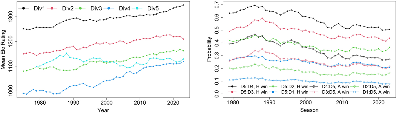
Average seasonal Elo ratings (strengths) since 1975 for English football’s top 5 leagues (left hand side), and the probability that a fifth division side would beat a team from the four higher divisions at home or away (right hand side).
In the three years of the existence of this rule, home teams won 46 % of matches, a little down from the 49–50 % in previous seasons – but not statistically significant. This is somewhat contrary, however, to Pollard (1986), who wrote (page 244): “As far as the scoring of points goes, home advantage has thus almost been eliminated by the new system.” Hence, whether the creation of an unbalanced point system giving a higher reward for an away win affected match outcomes is not clear.
There were small aggregate effects in final league standings from the two-point change. The Champions of the division would have been different in 1983/84 (Bath City rather than Wealdstone) and 1984/85 (Nuneaton Borough not Maidstone United) had the three-points for a win system not been altered. In 1985/86 the Champions would have been the same, but the relegation outcome would have differed (Dagenham, rather than Wycombe Wanderers, would have been relegated). On average, teams had 10 points fewer under the system, but on average final league positions were unaffected.[7]
2.3 Match Attendance
Whereas one might not expect too much concerning the effects on match outcomes this may have been different for match attendance. Football fans may or may not go to the stadium of the team they support. They may go to enjoy the match but they may also abstain from visiting the stadium for reasons not directly related to the expected performance of their team or the opponent. Buraimo, Migali, and Simmons (2016) for example analyzed the effects of a corruption scandal in Italian football in the 2005–06 season. Because some club officials were found to be guilty of corruption their clubs were punished typically by point deductions. Buraimo, Migali, and Simmons (2016) found that home attendance for the clubs involved in the corruption fell by about 16 % compared to the clubs who not punished. The authors concluded that the drop in attendance was not necessarily caused by moral disapproval of the home fans as a sign of protest. An alternative explanation is that the point deductions made it difficult for the clubs involved to end up high in the league. Thaler (1985) presented a theory of consumer choice in which mental accounting plays a role. In this theory the perceived fairness of a transaction is important. It may be that the setting of the two/three points system is perceived as unfair to potential buyers of seasonal tickets or individual match tickets. If so, stadium attendance would have suffered.
A novel strand of attendance demand literature in recent years has considered the concepts of shock, surprise and suspense, after the work of Ely, Frankel, and Kamenica (2015). Buraimo et al. (2020) found that shock and surprise have a positive effect on television demand, while Fischer et al. (2023) and Pawlowski et al. (2023) found suspense decreases complementary activities at football matches (alcohol sales and social media posting, respectively). We are unaware of any analyses considering shock, surprise and suspense on stadium attendance, but it is plausible that changes in shock, surprise and suspense levels caused by the perceived unfair reward system could affect demand.[8]
Finally, on the subject of unfairness, as already mentioned, APL clubs had to apply for election to the EFL, rather than achieving EFL status from finishing as champions. It is plausible that a failed election bid was perceived as unfair by supporters of that club, and hence reflected in attendances in the following season. Many supporters of football teams buy ‘season tickets’, bundles of tickets for an entire season, purchased before the season has begun. Such fans will make decisions based on outcomes of the previous season, such as a failed election bid. A final quirk of the system at the time is that the APL team put forward to be elected to the EFL was not necessarily the APL champion. In 1982 third placed Telford United were put forward, and in 1983 second placed Maidstone United were put forward.
3 Data
Our data is collected from two sources: for matches since 1999 from Soccerbase (www.soccerbase.com), and before 1999, Archives.football (www.thefootballarchives.com). It is the match results in terms of goals scored for each team, as well as in most cases the attendances (complete seasons through to 1990/91 hence covering the time period of interest).
The Soccerbase website is a well-regarded source of football-related data, having been used in numerous previous academic studies, and is operated by the Racing Post. The Archives.Football website is a more community-run site, where the website’s owner operates a ranking system for the veracity of information for each match. In the Football League, historical attendance numbers are known because of the need of clubs to report to the Football League for revenue sharing and tax purposes. At non-league level, attendances would be announced on the day, and recorded in matchday programs to be collected and referred to at a later point. There is no reason to believe that any measurement error would vary between the different periods we study in this paper.
In Figure 2 we plot seasonal average attendance data for English football’s top 5 leagues. The data show that across all the English football leagues, the mid-1980s were the low point in demand for football attendance, most likely as a result of poor economic circumstances in England (Reade and Van Ours 2023). After the 1986/87 season, relegated clubs from the EFL begin to enter the dataset with much greater attendances than the clubs that previously existed in the APL. Therefore, we end our sample at the end of the 1986/87 season. We limit our comparison to a small number of seasons either side so that the ‘control group’ is similar to the ‘treatment group’. Therefore, the first season in our sample is 1979/80 at the time when a win counted for two points.
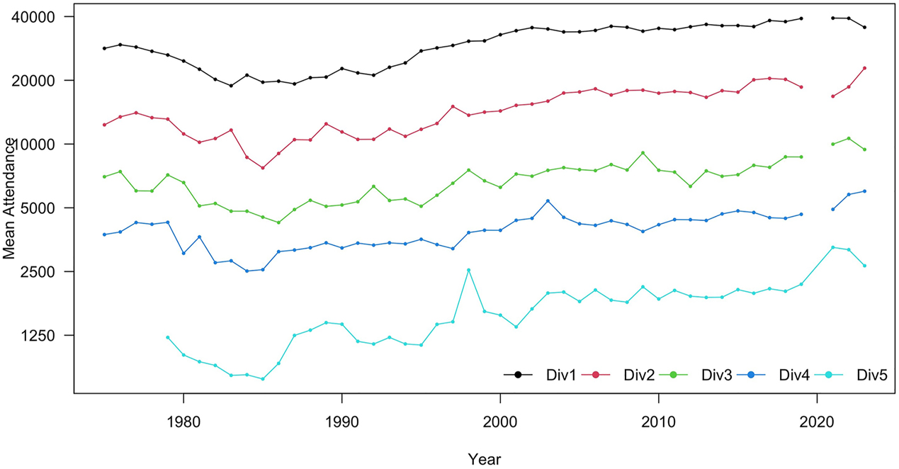
Average seasonal attendances (log scale) since 1975 for English football’s top 5 leagues.
In Table 1 we present summary statistics for our eight seasons in full, which amounts to 3,532 observations. Home teams score around half a goal more than away teams, and there is almost three goals a game, on average. Home teams win around 47 % of the time, away teams 27 % of the time, with about 26 % of matches ending as draws. Forecast outcomes are based on the Elo rating system (Elo 1978), a well-known system devised for chess and commonly applied across many sports including football (e.g. Hvattum and Arntzen 2010; Reade and Garcia-del Barrio 2023). The forecast outcomes are, on average, quite close to reality, with the average home win probability being 47 %, and 28 % for the away win. Expected home points are 1.4 over the sample, and expected away points are about one. The average attendance over the sample period is 915, just under a thousand, while the local areas (local authorities or districts) around the football clubs in the APL over this period is about 150 thousand people. Finally, this nationwide competition had, on average, teams travelling about 114 miles to reach away matches.
Summary statistics.
| Statistic | N | Mean | St. dev. | Min | Pctl(25) | Pctl(75) | Max |
|---|---|---|---|---|---|---|---|
| Home goals | 3,532 | 1.688 | 1.386 | 0 | 1 | 2 | 8 |
| Away goals | 3,532 | 1.183 | 1.107 | 0 | 0 | 2 | 6 |
| Total goals | 3,532 | 2.871 | 1.793 | 0 | 2 | 4 | 11 |
| Goal difference | 3,532 | 0.504 | 1.755 | −5 | −1 | 2 | 8 |
| Home win outcome | 3,532 | 0.474 | 0.499 | 0 | 0 | 1 | 1 |
| Draw outcome | 3,532 | 0.259 | 0.438 | 0 | 0 | 1 | 1 |
| Away win outcome | 3,532 | 0.267 | 0.442 | 0 | 0 | 1 | 1 |
| Probability of home win | 3,532 | 0.471 | 0.102 | 0.059 | 0.398 | 0.542 | 0.781 |
| Probability of draw | 3,532 | 0.253 | 0.023 | 0.103 | 0.242 | 0.271 | 0.274 |
| Probability of away win | 3,532 | 0.276 | 0.083 | 0.083 | 0.215 | 0.329 | 0.838 |
| Expected home team points | 3,532 | 1.380 | 0.325 | 0.220 | 1.142 | 1.571 | 2.452 |
| Expected away team points | 3,532 | 1.022 | 0.276 | 0.302 | 0.825 | 1.205 | 2.618 |
| Attendance (1,000s) | 3,532 | 9.147 | 0.441 | 0.121 | 0.61 | 0.110 | 0.5640 |
| Population local area home team (100,000s) | 3,532 | 1.564 | 0.902 | 0.509 | 0.923 | 2.206 | 5.050 |
| Distance (100s of miles) | 3,532 | 1.135 | 0.576 | 0.040 | 0.702 | 1.501 | 3.023 |
Figure 3 shows the evolution over our sample period of the expected points for home teams and away teams. Panel (a) shows the expected points per match, panel (b) shows the seasonal average difference in expected points for home teams minus away teams. Both figures clearly show the implications of the change in the points system. Obviously in the seasons with three points for a win the expected numbers of points are higher for both home and away teams in comparison with the seasons with two points for a win. In the three seasons with fewer points for a home win the difference in expected points between home teams and away teams is very small. In other words, the home advantage in terms of expected points in these three seasons almost disappeared.
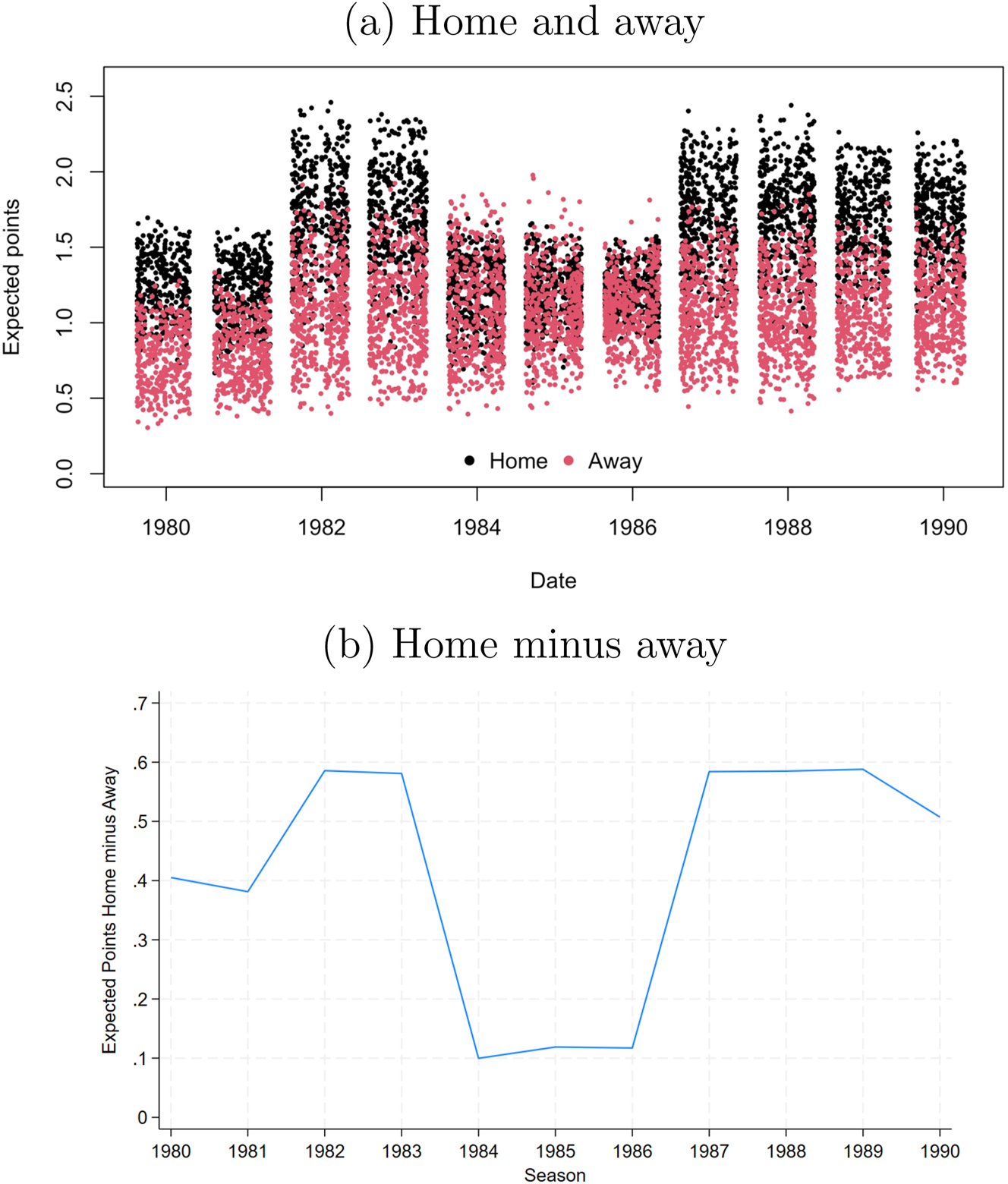
Expected points per match. (a) Home and away. (b) Home minus away.
In Table 2 we break the means of these variables into the four separate time periods under consideration. In 1979–81 each team got two points for a win, in 1981–83 both teams got three points for a win, in 1983–86 only the away team got three points for a win, and in 1986/87 both teams got three points for a win again. Each column is the mean for that variable for that sub period, with stars indicating the statistical significance of a difference in means test.[9] In 1981–83, total goals increase from 2.66 to 2.93, with 0.18 of that for the home team, and 0.09 for the away team. These differences are statistically significant, but they did not result in more wins for the home team, statistically, as that proportion changed from 49 % (1979–81) to 50 % (1981–83). When the reward for home teams fell back to two points, home goals fell back, on average, by 0.1 of a goal, and away goals increased by a further 0.06. This brought the proportion of home (away) wins down (up) to 46 % (28 %) from 50 % (25 %) but these changes are not significant. Considering expected points, these were 1.2 and 0.8 for the home and away teams respectively in 1979–81, and rose to 1.67 and 1.08 in 1981–83 with three points for a win. In 1983–86 the home team’s expected points fell back to essentially their previous level (1.19) and away expected points remained at 1.08. As such, the expected difference in points was 0.4 in 1979–81, 0.6 in 1981–83, then 0.1 in 1983–86, and back to 0.6 in 1986/87. Attendances were falling throughout much of this period, dropping from 1,115 in 1979–81 to 919 in 1981–83, then further to 800 in 1983–86 before recovering to 921 in 1986/87.
Means of main variables for different sub-periods of our data sample.
| 1979–81 | 1981–83 | 1983–86 | 1986/87 | |
|---|---|---|---|---|
| Home goals | 1.59 | 1.77*** | 1.67 | 1.73* |
| Away goals | 1.07 | 1.16* | 1.22*** | 1.31*** |
| Total goals | 2.66 | 2.93*** | 2.89*** | 3.03*** |
| Goal difference | 0.53 | 0.61 | 0.45 | 0.42 |
| Home win outcome | 0.49 | 0.50 | 0.46 | 0.45 |
| Draw outcome | 0.27 | 0.25 | 0.26 | 0.25 |
| Away win outcome | 0.25 | 0.25 | 0.28 | 0.30* |
| Probability of home win | 0.47 | 0.47 | 0.47 | 0.47 |
| Probability of draw | 0.25 | 0.25 | 0.25 | 0.26* |
| Probability of away win | 0.28 | 0.28 | 0.28 | 0.28 |
| Expected home team points | 1.20 | 1.67*** | 1.19 | 1.66*** |
| Expected away team points | 0.80 | 1.08*** | 1.08*** | 1.08*** |
| Attendance (1,000s) | 1.11 | 0.92*** | 0.80*** | 0.92*** |
| Population local area home team (100,000s) | 1.37 | 1.64*** | 1.59*** | 1.65*** |
| Distance (100s of miles) | 1.13 | 1.14 | 1.15 | 1.10 |
| Reward winning match (points): home win | 2 | 3 | 2 | 3 |
| Away win | 2 | 3 | 3 | 2 |
-
Note: *p < 0.1; ∗∗∗p < 0.01.
Figure 4 shows that over the seasons 1979/80 to 1989/90 the likelihood of a home win did not change very much while the probability of an away win increased somewhat. Over the three seasons of our main interest the win probabilities do not seem to be very different from the seasons before or after. Figure 4 also shows the development of seasonal attendances where over the three seasons of our main interest these are lower than in the seasons before and after.
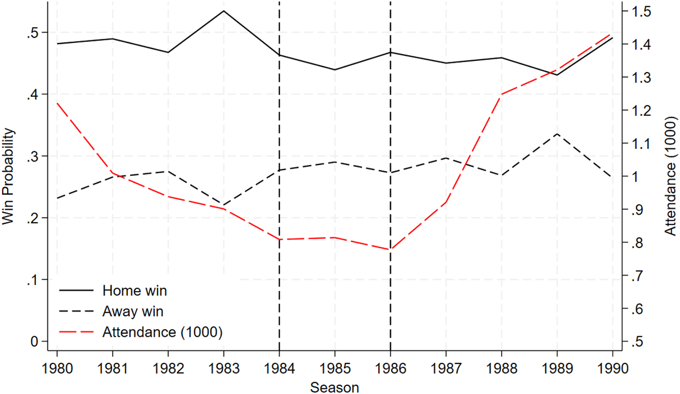
Win probabilities and seasonal attendances; 1979/80–1989/90.
4 Methodology
We first consider simple linear models in a number of match outcome variables to see if there was any measured and significant impact of the rule change. Our unit of analysis is the match level, and hence we think about matches between home team i, and visiting team j at time t. Because we consider many seasons, we have a significant number of repeat observations. Our dependent variables are:
Goals by the home (away) team, team i (j), denoted gi ijt (gj ijt ).
Home win:
Draw:
Away win:
We include a small number of other explanatory variables to control for any remaining variation in our dependent variables:
Elo prediction, elo ijt : This is a variable that takes any value on the unit interval, where 0 implies that the away team is certain to win, and 1 implies the home team will certainly win.
Wins per game, wpg it and wpg jt . Elo ratings are one measure of the quality of teams involved in matches, and they are a function of match outcomes weighted for the quality of the opposition. A simpler measure is just to look at the wins a team achieves. Because wins will accumulate over a season, we take wins per game, which is the ratio of wins at any point in a season to the number of matches played so far.
Form, form it and form jt : While wins are a season-level measure, being reset to zero at the start of each season, Form is a more temporary measure of team quality, and is conventionally the number of points achieved in a team’s most recent matches. We take the six most recent matches.[10]
We also include fixed effects for home and away teams and the gameweek of the season in order that any effect we see cannot be attributed to different teams. We cannot include season fixed effects as we seek to identify an effect that only existed at a seasonal level.
Our explanatory variables of interest are:
Two Home Points Rule, 2hpr t : This is a variable taking the value 1 for the seasons when a home team only received two points for a win while the away team received three points if they won. That is, for the seasons 1983/84, 1984/85 and 1985/86 this variable takes the value 1.
Three Points Rule, 3pr t : This variable takes the value 1 for the seasons where both teams received three points for a win. That is, season 1981/82, 1982/83, and 1986/87 in our sample.
We are mainly interested in the first of these two ‘treatment’ variables, but given that three points for a win was a significant structural change in English football, we also include this to consider whether it had any impact.
Our first set of regression models are thus:
Having looked at match outcomes, we then consider attendances. The attendance data need to be thought of within the context of English football – at the time the game was struggling, with declining attendances continually since the postwar boom. The low point for EFL attendances was 1986, the point at which the experiment ended (and promotion/relegation was introduced). With our modelling we follow the same approach as Humphreys and Zhou (2015) and Coates, Humphreys, and Zhou (2014) who brought in a range of theories regarding fan, or consumer behaviour.
As such, we model log attendance on measures to capture fan preferences for the home win, for quality, for a number of aspects of competitive balance, and for loss aversion. We don’t have information on ticket prices at the time. Dobson and Goddard (2004) provided a set of price indices for the Football League divisions. We included the Fourth Division price index but find that it makes no difference to our regression results and the coefficients are insignificant. Furthermore, we do not have information about hooliganism or weather conditions both of which may have affected attendances. Incidents of hooliganism or bad weather may have had a negative influence on attendance. However, we think that in the context of our analysis not including hooliganism or weather as explanatory variables may not the very important. It would have been if hooliganism would have been more severe or weather would have been worse during the seasons 1983/84 to 1985/86 than they were during earlier or later seasons. Although we cannot rule this out we think it is not very likely. We also do not have information about ground capacity. However, we think that this is not problematic as in our period of analysis attendances had been declining for some time so capacity constraints are unlikely to be important.
We run:
Here:
A ijt : Recorded attendance of match between team i and j at time t.
p ijt : Probability of home win (team i). This is calculated using a multinomial logit model that includes the Elo prediction, the points earned per game, the goal difference per game, and the form (points in the last six matches), all for each team. As per Humphreys and Zhou (2015) we correct for the impact of team quality in this measure, given that is an additional variable in the model. We do this by regressing the probabilities on the quality variables and using the residuals from that regression.
P T : Price of attending a football match. As mentioned above, price data is very hard to find in football, especially back to the 1980s in non-league football. As such we are unable to include P T in our empirical model. We include, where possible, measures that proxy the cost of attending, most notably the distance between the two clubs competing in a match.
LS t : The League Standing Effect, as coined by Neale (1964). This is the total number of position changes in the leagues standings after the most recent set of matches in the division. This is one of the measures that Humphreys and Zhou (2015) used to account for the League Standing Effect.
Q i , Q j : Team quality. We measure this using the league position of each team before each match.[11] We consider seasonal measures of team quality also, since a proportion of attendees at any match will have purchased a season ticket, a bundle of tickets for the entire season, purchased before the season began, based on information from the previous season. We include the previous season’s league position, and a dummy for whether the team was champion.
D t : Matchday-specific characteristics. Here, we include dummy variables for the day of the week as midweek evening matches tend to have lower attendances. We also include the physical distance, in miles, between the two teams. This can only be included when we include home and away team fixed effects. When we use match-up fixed effects the distance variable drops out.
The expected home win probability ignores the probability of a draw occurring. Empirically about 25 % of all matches end in a draw. Therefore, Besters, Van Ours, and Van Tuijl (2019) used as an alternative measure match expectation, defined as the expected number of points for the home team. They found that this measure outperforms home win probability. As shown in panel b of Figure 3 the number of expected points is much lower in the two-points-for-a-home-win three-points-for-an-away-win period. In fact the home advantage as measured through the expected number of points for the home team almost disappears. This also implies that there is a high correlation between the dummy variable “Seasons with 2 points for a home win” and the number of expected points. Therefore, we did not include the expected number of points as explanatory variable.
Additionally, we employ an event study approach to consider the impact in the games immediately after the rules were introduced (and abandoned). We include a time trend for home match of the season in our event studies, in order to control for the fact that there is natural variation across the season.
In this case, our generic model for the three different policy periods (introduction of three points for a win, introduction of two points for a home win, end of two points for a home win):
In (3) X ijt is a set of explanatory variables almost identical to those included in (2). We estimate (3) up to the 20th match of the three seasons where rule changes occurred – 1981/82, 1983/84 and 1986/87.
5 Results
We firstly consider the extent to which the new rule impacted match outcomes. In Table 3 we regress match outcomes (home win, draw, away win), goals scored by the home and away team, the total goals scored and difference in goals scored, on variables that might explain that, as well as dummy variables for the new points regimes (3 points for a win in 1981/82 and 1982/83, 2/3 points for a win in 1983/84, 1984/85 and 1985/86, and back to 3 points for a win in 1986/87). We also include fixed effects for the home and away team in a match as well as the gameweek of the season, and cluster standard errors at the home team and season level.[12]
Regression results considering major match outcome variables.
| Dependent variable | |||||||
|---|---|---|---|---|---|---|---|
| Outcome | Goals | ||||||
| Home win | Draw | Away win | Home | Away | Total | Difference | |
| (1) | (2) | (3) | (4) | (5) | (6) | (7) | |
| Elo prediction | 0.147 | 0.041 | −0.188 | 0.862** | −0.164 | 0.698 | 1.025** |
| (0.139) | (0.118) | (0.125) | (0.316) | (0.203) | (0.420) | (0.326) | |
| Three points rule | 0.005 | −0.007 | 0.002 | 0.175* | 0.114* | 0.289* | 0.062 |
| (0.025) | (0.022) | (0.020) | (0.083) | (0.057) | (0.136) | (0.054) | |
| Two home points rule | −0.023 | 0.004 | 0.019 | 0.056 | 0.092* | 0.147* | −0.036 |
| (0.019) | (0.026) | (0.018) | (0.052) | (0.046) | (0.066) | (0.053) | |
| Wins per game (home) | 0.119 | 0.011 | −0.130** | 0.159 | −0.359* | −0.200 | 0.518* |
| (0.067) | (0.045) | (0.046) | (0.226) | (0.160) | (0.297) | (0.257) | |
| Wins per game (away) | −0.079 | 0.080 | −0.001 | −0.297** | −0.109 | −0.406* | −0.188 |
| (0.064) | (0.076) | (0.073) | (0.120) | (0.122) | (0.185) | (0.158) | |
| Form (home) | 0.004 | −0.001 | −0.004 | 0.009 | −0.005 | 0.004 | 0.015 |
| (0.005) | (0.003) | (0.003) | (0.012) | (0.017) | (0.019) | (0.018) | |
| Form (away) | −0.005 | −0.002 | 0.008 | −0.019*** | 0.008 | −0.011 | −0.026* |
| (0.004) | (0.002) | (0.004) | (0.004) | (0.010) | (0.010) | (0.012) | |
| Observations | 3,532 | 3,532 | 3,532 | 3,532 | 3,532 | 3,532 | 3,532 |
| R 2 | 0.075 | 0.024 | 0.071 | 0.088 | 0.071 | 0.056 | 0.109 |
| Adjusted R2 | 0.051 | −0.001 | 0.047 | 0.064 | 0.047 | 0.031 | 0.086 |
| Residual std. error (df = 3,442) | 0.487 | 0.439 | 0.432 | 1.341 | 1.080 | 1.765 | 1.678 |
-
Note: *p
Our estimations are over all the seasons up until the end of 1986/87 season, hence eight seasons and 3,532 matches. The impact of the two-points home win rule is represented by the “Two home points rule” row in the table. The impact of the two home points rule is insignificant on match outcomes in the first three columns of the table.
Home goals and away goals are slightly more likely than before the two-home-points period, and away goals a little more likely (about 0.11 more away goals on average). Total goals are thus also more likely, and the goal difference is smaller. Only the away goals and total goals impacts are significant, and even then only at the 10 % level.
The three points rule had a more significant impact on goals but not on outcomes. Home goals became more likely by at least 0.14 on average, and away goals by about 0.16 in 1981, and then by about 0.24 in 1986, with the cumulative effect on total goals showing via the total goals column (6). The goal difference appears to have been affected, increasing during each three-point period via the expected points difference coefficient, but this effect is not significant.
As such, we are left to conclude that the impact on match outcomes was not dramatic, even if we can see changes in the raw numbers from Table 2. Controlling for team quality renders these effects mostly insignificant.
If we in turn consider attendances at these matches, we can see from regression results in Table 4 that there was an impact. These regressions all have fixed effects for the day of the week and the month of the season, as well as team-specific fixed effects which are indicated in the ‘FE’ row. If we consider our constructed probability of a home win to be a good predictor of how competitive a match is and hence how interesting, then in the first column we see that attendances were around 17 % lower during the three seasons of the two home points experiment. Adding in more salient measures of home and away team quality and allowing for habit formation by introducing lagged attendance in the second column reduces the size of the effect to around 11 %, but it remains significant. We find evidence of habit formation as lagged attendance has a significant and positive effect.
Regression results considering attendance.
| Dependent variable | ||||||||
|---|---|---|---|---|---|---|---|---|
| Log attendance | ||||||||
| (1) | (2) | (3) | (4) | (5) | (6) | (7) | (8) | |
| Lag log attendance | 0.410*** | 0.408*** | 0.457*** | 0.457*** | 0.387*** | 0.389*** | 0.383*** | |
| (0.052) | (0.052) | (0.060) | (0.059) | (0.031) | (0.031) | (0.030) | ||
| Win in last home game | 0.085*** | 0.085*** | 0.077*** | 0.077*** | 0.073*** | 0.073*** | 0.073*** | |
| (0.008) | (0.008) | (0.009) | (0.009) | (0.006) | (0.006) | (0.006) | ||
| P(H) | 0.918*** | −0.889** | −0.842** | −0.647** | −1.320*** | −1.380*** | ||
| (0.101) | (0.298) | (0.303) | (0.185) | (0.363) | (0.354) | |||
| P(H)2 | 0.791** | 0.755** | 0.556** | 1.504*** | 1.551*** | |||
| (0.313) | (0.318) | (0.183) | (0.427) | (0.416) | ||||
| Corrected P(H) | −0.183* | 0.056 | ||||||
| (0.080) | (0.087) | |||||||
| Corrected P(H)2 | 1.140* | 1.265** | ||||||
| (0.559) | (0.469) | |||||||
| Position (home) | −0.014*** | −0.014*** | −0.013*** | −0.012*** | −0.012*** | −0.012*** | −0.012*** | |
| (0.001) | (0.001) | (0.001) | (0.002) | (0.001) | (0.001) | (0.001) | ||
| Position (away) | −0.006*** | −0.006*** | −0.004*** | −0.005*** | −0.006*** | −0.005*** | −0.006*** | |
| (0.001) | (0.001) | (0.001) | (0.001) | (0.001) | (0.001) | (0.001) | ||
| League position changes | 0.004*** | 0.004*** | 0.004** | 0.004** | 0.004*** | 0.003*** | 0.004*** | |
| (0.001) | (0.001) | (0.001) | (0.001) | (0.001) | (0.001) | (0.001) | ||
| Distance | −0.001*** | −0.001*** | ||||||
| (0.0002) | (0.0002) | |||||||
| Population (home) | 0.002 | 0.003 | 0.002 | 0.002 | −0.0004 | −0.0004 | −0.00002 | |
| (0.004) | (0.004) | (0.004) | (0.005) | (0.001) | (0.001) | (0.001) | ||
| Population (away) | 0.002 | 0.003 | 0.002 | 0.002 | −0.0005 | −0.0005 | −0.0001 | |
| (0.002) | (0.002) | (0.001) | (0.001) | (0.001) | (0.001) | (0.001) | ||
| Seasons with 3 points for a win | −0.048 | −0.034 | −0.038 | −0.038 | −0.023 | −0.026 | −0.051 | |
| (0.039) | (0.038) | (0.035) | (0.034) | (0.045) | (0.045) | (0.035) | ||
| Seasons with 2 points for home win | −0.170*** | −0.116** | −0.098** | −0.098** | −0.098** | −0.146*** | −0.148*** | −0.126*** |
| (0.042) | (0.041) | (0.039) | (0.035) | (0.035) | (0.043) | (0.044) | (0.044) | |
| Season (time trend) | −0.005 | −0.004 | −0.004 | 0.007*** | 0.007*** | 0.004 | ||
| (0.006) | (0.005) | (0.005) | (0.002) | (0.002) | (0.003) | |||
| Seasons with 1 promotion spot | 0.094* | |||||||
| (0.053) | ||||||||
| Seasons with 2 promotion spots | 0.038 | |||||||
| (0.035) | ||||||||
| Last season’s final position | −0.003** | −0.003* | −0.003** | −0.003** | −0.003*** | −0.003*** | −0.004*** | |
| (0.001) | (0.001) | (0.001) | (0.001) | (0.001) | (0.001) | (0.001) | ||
| Champions previous season | −0.030* | −0.031* | −0.033* | −0.036 | −0.053*** | −0.055*** | −0.040** | |
| (0.013) | (0.014) | (0.017) | (0.020) | (0.013) | (0.012) | (0.019) | ||
| Denied election to FL last summer | 0.038** | 0.041*** | 0.041** | 0.041** | 0.072*** | 0.075*** | 0.064** | |
| (0.013) | (0.011) | (0.017) | (0.017) | (0.020) | (0.020) | (0.025) | ||
| Observations | 3,532 | 3,502 | 3,502 | 3,502 | 3,502 | 14,079 | 14,079 | 14,079 |
| R 2 | 0.626 | 0.774 | 0.774 | 0.850 | 0.850 | 0.913 | 0.912 | 0.913 |
| Adjusted R2 | 0.617 | 0.767 | 0.768 | 0.797 | 0.797 | 0.872 | 0.871 | 0.872 |
| Residual std. error | 0.286 (df = 3,452) | 0.223 (df = 3,409) | 0.222 (df = 3,408) | 0.208 (df = 2,581) | 0.208 (df = 2,581) | 0.229 (df = 9,599) | 0.229 (df = 9,599) | 0.228 (df = 9,597) |
| FE | t1 + t2 | t1 + t2 | t1 + t2 | t1 × t2 | t1 × t2 | t1 × t2 | t1 × t2 | t1 × t2 |
| Seasons | 1979–1986 | 1979–1986 | 1979–1986 | 1979–1986 | 1979–1986 | 1979–2020 | 1979–2020 | 1979–2020 |
-
Note: *p
We include season-level measures also to account for season-ticket holders who make their purchase decisions each summer based on the previous season. One league position higher the previous season leads to a small increase in attendance the season after (about 0.3 %). Being champion the previous season, in a time period when the champion was not necessarily promoted, decreases attendances by between 3 and 5 %. Each club that was put forward for election to the Football League between 1979 and 1986 was not elected, and hence we can see whether that decision led to fans making different decisions about attending. That is, we test whether another perceived source of unfairness could adversely impact attendances. Conversely, we find that a failed election bid increases attendances by around 4 %. This may be an effect akin to that of failed Olympic bid host cities, who experience similar positive economic impacts to cities selected to host (Rose and Spiegel 2011). Hence rather than fans seeing a failed election attempt as an off-putting unfairness, more broadly that election attempt sends a signal to a club’s fanbase that the club is ambitious and seeking the prestigious EFL status.
The introduction of a time trend in the third column to capture the reality that attendances at English football were declining over the time period does reduce the impact to about 9 %.[13] In the fourth column we introduce match-up fixed effects rather than separate fixed effects for the two teams, and this has no impact on the size of the effect.[14] In the fifth column we use corrected probabilities of a home win (removing the effect of team quality on the probability in order that it only reflects uncertainty of outcome). Doing this has no impact on any of the coefficients in the model, and the effect of the two-home-points season remains at about 10 %.
In the final three columns we extend estimation through to the point that the league stopped for Covid-19 in March 2020; in column (6) we repeat the regression of column (4) for the longer sample, in column (7) we extend the regression in column (5) and in column (8) we add dummies for the seasons with one promotion spot to the EFL (1986/87 onwards), and two promotion spots (2003/04 onwards). Neither are significant. The impact of the two-home-points rule is notably larger when we estimate over the longer sample. However, attendances were more broadly rising in English football over the entire period after the mid-1980s, which likely accounts for much of this larger effect.
As a robustness check on our findings, we run ‘placebo’ regressions presented in Table A.2 in the Appendix, in which for comparison the first column shows the parameter estimates for the APL (see also Table 4). We run exactly the same regression as reported as in the first column but we estimate instead over the Second, Third and Fourth Divisions of the EFL, the divisions above the APL. These divisions were treated to the three-point rule, but not the two-point-home rule, and this is reflected as the two-point-home rule coefficient is insignificant in each of these regressions.
Our event study outcomes are shown in Figure 5. In the middle panel we plot the impact of the two-home-points rule. To the left of the vertical solid line we plot the ten matches before the rule was introduced, which are all insignificantly different from zero. Immediately after the solid vertical line, where the two-home-points rule was introduced, attendances fall, and in the second and third gameweeks after the change they are almost 20 % lower than previously. Through to gameweek 15 attendances are between 5 and 15 % lower than before the rule change was introduced.
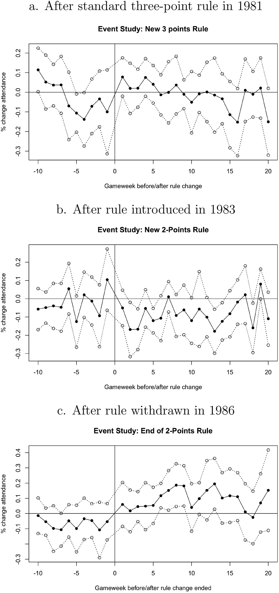
Impact on matchday attendances of change in rules. (a) After standard three-point rule in 1981. (b) After rule introduced in 1983. (c) After rule withdrawn in 1986.
In the bottom plot, the rule was abandoned where the solid vertical line is plotted. Again, in the ten games prior to the rule’s abandonment, attendances are not significantly different from zero, although all coefficients are negative.[15] To the right of the solid line, once the rule was abandoned, attendances began to rise, and between gameweeks 6 and 10 attendances are significantly higher than before the rule was abandoned. For the remainder of the post-policy period, attendances are about 10 % higher than they were when the rule was still in place.
The top panel plots attendances in and around the 3-point-for-a-win introduction in 1981 in the same format as the other plots. There is no noticeable impact on attendances in this plot.
6 Conclusions
We investigate a novel tweak on a known rule change in football. Rather than rewarding a win with three points under this anomalous rule change three points were rewarded for an away win but only two for a home win. The rule change affected the rewards from effort, and literature has shown that the change had an ambiguous impact due to it affecting both the reward from effort and also the reward from sabotage (increasing opponent costs of effort). The two-points-for-a-home-win and three-points-for-an-away-win was abolished after three seasons. The reasons of the introduction of the anomalous point system are not fully clear and neither are the reasons for abolishing the system.
We find that this particular tweak, which affected only the home side but not the away side, had a negative impact on attendances, though not on measurable match outcomes. It could be that clubs realized that match outcomes were not affected but it seems unlikely that clubs were aware of the drop in match attendance. In the early 1980s attendances in English professional football were still falling. Therefore, the drop in attendance due to the anomalous point system may have gone unnoticed. Otherwise, it would not have lasted three years before the system was abolished and fairness of rewarding wins was restored.
Our main finding is that the unbalanced rewarding of home wins and away wins reduced stadium attendance. The negative attendance effects are clearly present as are the positive effects of restoring the three-points-for-a-win system. As the style of play was not affected the attendance effects are not driven by a change in the nature of the games. We can only speculate about the nature of the attendance effect. It could be that potential attendants expected the away team to attack more and therefore the home team would be more likely to lose a match. If the potential attendants were loss-averse they would not come to the stadium. It also could be that the differences in win-reward-points between away teams and home teams affected the perception of potential stadium visitors. The new system may have been perceived as unfair to the home team. As a response to this perception potential visitors decided to avoid watching the game in person. We think that the latter interpretation is more appropriate as potential attendants would have observed (after a while) that match outcomes did not change because of the new system but the perceived unfairness remained.
-
Competing interests: The authors declare that they have no known competing financial interests or personal relationships that could have appeared to influence the work reported in this paper. They thank two anonymous reviewers for helpful comments on a previous version of the paper. The data used in the analysis will be made available through a public access website.
Appendix A: Additional Parameter Estimates
A.1 Outcomes
Regression results considering major match outcome variables where Probit regression models are used for outcomes, and Poisson regression models are used for the count variables.
| Dependent variable | |||||||
|---|---|---|---|---|---|---|---|
| Outcome | Goals | ||||||
| Home win | Draw | Away win | Home | Away | Total | Difference | |
| Probit | Probit | Probit | Poisson | Poisson | Poisson | Poisson | |
| (1) | (2) | (3) | (4) | (5) | (6) | (7) | |
| Constant | −0.184 | −0.823*** | −0.388 | 0.156 | 0.240 | 0.900*** | 2.502*** |
| (0.258) | (0.276) | (0.280) | (0.156) | (0.187) | (0.119) | (0.059) | |
| Elo prediction | 0.491 | −0.016 | −0.534 | 0.563** | −0.151 | 0.266 | −0.100 |
| (0.380) | (0.404) | (0.412) | (0.228) | (0.274) | (0.175) | (0.088) | |
| Three points rule | −0.001 | −0.0004 | −0.010 | 0.087** | 0.090* | 0.089*** | −0.004 |
| (0.067) | (0.071) | (0.073) | (0.041) | (0.050) | (0.032) | (0.016) | |
| Two home points rule | −0.069 | 0.028 | 0.050 | 0.031 | 0.079 | 0.052 | 0.003 |
| (0.067) | (0.071) | (0.073) | (0.041) | (0.050) | (0.032) | (0.015) | |
| Wins per game (home) | 0.280* | 0.060 | −0.455** | 0.099 | −0.283** | −0.050 | −0.042 |
| (0.162) | (0.171) | (0.185) | (0.095) | (0.121) | (0.075) | (0.038) | |
| Wins per game (away) | −0.214 | 0.264 | 0.008 | −0.203** | −0.084 | −0.151** | 0.019 |
| (0.161) | (0.168) | (0.173) | (0.100) | (0.115) | (0.075) | (0.037) | |
| Form (home) | 0.013 | −0.003 | −0.011 | 0.010** | −0.002 | 0.005 | −0.002 |
| (0.008) | (0.009) | (0.009) | (0.005) | (0.006) | (0.004) | (0.002) | |
| Form (away) | −0.012 | −0.010 | 0.024*** | −0.005 | 0.009 | 0.001 | 0.002 |
| (0.008) | (0.009) | (0.009) | (0.005) | (0.006) | (0.004) | (0.002) | |
| Observations | 3,532 | 3,532 | 3,532 | 3,532 | 3,532 | 3,532 | 3,532 |
| Log likelihood | −2,311.704 | −1,986.381 | −1,927.180 | −5,665.984 | −4,863.991 | −6,811.905 | −7,998.257 |
| Akaike inf. crit. | 4,765.407 | 4,114.761 | 3,996.361 | 11,473.970 | 9,869.982 | 13,765.810 | 16,138.510 |
-
Note: *p
A.2 Attendance
Regression results from running placebo models, regressing attendances at divisions two, three and four levels over the same period as the two-points-for-a-home-win experiment.
| Dependent variable: log attendance | ||||
|---|---|---|---|---|
| APL | Div 4 | Div 3 | Div 2 | |
| (1) | (2) | (3) | (4) | |
| Lag log attendance | 0.413*** | 0.286*** | 0.380*** | 0.321*** |
| (0.053) | (0.040) | (0.026) | (0.020) | |
| Win in last home game | 0.082*** | 0.091*** | 0.090*** | 0.088*** |
| (0.009) | (0.010) | (0.011) | (0.011) | |
| P(H) | −0.704** | −2.693** | −2.040* | −2.360*** |
| (0.215) | (0.834) | (0.956) | (0.523) | |
| P(H) squared | 0.724** | 2.884** | 2.389* | 2.522*** |
| (0.214) | (0.883) | (1.024) | (0.585) | |
| Position (home) | −0.013*** | −0.014*** | −0.015*** | −0.022*** |
| (0.002) | (0.001) | (0.001) | (0.001) | |
| Position (away) | −0.006*** | −0.011*** | −0.011*** | −0.011*** |
| (0.001) | (0.001) | (0.001) | (0.001) | |
| League position changes | 0.004*** | 0.003* | 0.004** | 0.006** |
| (0.001) | (0.002) | (0.001) | (0.002) | |
| Distance | −0.001*** | −0.002*** | −0.002*** | −0.002*** |
| (0.0001) | (0.0001) | (0.0001) | (0.0001) | |
| Population (home) | 0.003 | 0.002 | −0.001 | −0.001 |
| (0.006) | (0.002) | (0.002) | (0.002) | |
| Population (away) | 0.002 | 0.003* | −0.001* | −0.002 |
| (0.002) | (0.001) | (0.001) | (0.002) | |
| Seasons with 3 points for a win | −0.058 | −0.075** | −0.104*** | −0.045* |
| (0.048) | (0.022) | (0.024) | (0.021) | |
| Seasons with 2 points for home win | −0.071*** | −0.051 | −0.037 | −0.041 |
| (0.014) | (0.053) | (0.032) | (0.022) | |
| Observations | 3,504 | 2,876 | 3,822 | 3,469 |
| R 2 | 0.772 | 0.836 | 0.790 | 0.782 |
| Adjusted R2 | 0.766 | 0.828 | 0.783 | 0.775 |
| Residual std. error | 0.223 (df = 3,414) | 0.228 (df = 2,750) | 0.234 (df = 3,694) | 0.245 (df = 3,359) |
-
Note: *p
References
Besters, L. M., J. C. Van Ours, and M. A. Van Tuijl. 2019. “How Outcome Uncertainty, Loss Aversion and Team Quality Affect Stadium Attendance in Dutch Professional Football.” Journal of Economic Psychology 72: 117–27. https://doi.org/10.1016/j.joep.2019.03.002.Search in Google Scholar
Bloyce, D., and P. Murphy. 2008. “Sports Administration on the Hoof: The Three Points for a Win ‘Experiment’ in English Soccer.” Soccer and Society 9 (1): 14–27. https://doi.org/10.1080/14660970701616688.Search in Google Scholar
Brocas, I., and J. D. Carrillo. 2004. “Do The “Three-Point Victory” and “Golden Goal” Rules Make Soccer More Exciting?” Journal of Sports Economics 5 (2): 169–85. https://doi.org/10.1177/1527002503257207.Search in Google Scholar
Buraimo, B., D. Forrest, I. McHale, and J. Tena. 2020. “Unscripted Drama: Soccer Audience Response to Suspense, Surprise, and Shock.” Economic Inquiry 58 (2): 881–96. https://doi.org/10.1111/ecin.12874.Search in Google Scholar
Buraimo, B., G. Migali, and R. Simmons. 2016. “An Analysis of Consumer Response to Corruption: Italy’s Calciopoli Scandal.” Oxford Bulletin of Economics & Statistics 78 (1): 22–41. https://doi.org/10.1111/obes.12094.Search in Google Scholar
Butler, D., and R. Butler. 2017. “Rule Changes and Incentives in the League of Ireland from 1970 to 2014.” Soccer and Society 18 (5–6): 785–99. https://doi.org/10.1080/14660970.2016.1230347.Search in Google Scholar
Che, X., and B. Humphreys. 2015. “Competition between Sports Leagues: Theory and Evidence on Rival League Formation in North America.” Review of Industrial Organization 46 (2): 127–43. https://doi.org/10.1007/s11151-014-9439-7.Search in Google Scholar
Coates, D., B. R. Humphreys, and L. Zhou. 2014. “Reference-Dependent Preferences, Loss Aversion, and Live Game Attendance.” Economic Inquiry 52 (3): 959–73. https://doi.org/10.1111/ecin.12061.Search in Google Scholar
Dobson, F., and J. Goddard. 2004. “Revenue Divergence and Competitive Balance in a Divisional Sports League.” Scottish Journal of Political Economy 51 (3): 359–76. https://doi.org/10.1111/j.0036-9292.2004.00310.x.Search in Google Scholar
Elo, A. E. 1978. The Rating of Chessplayers, Past and Present, Vol. 3. London: Batsford.Search in Google Scholar
Ely, J., A. Frankel, and E. Kamenica. 2015. “Suspense and Surprise.” Journal of Political Economy 123 (1): 215–60. https://doi.org/10.1086/677350.Search in Google Scholar
Fischer, L., A. Kelava, M. Nagel, and T. Pawlowski. 2023. Celebration Beats Frustration: Emotional Cues and Alcohol Use During Soccer Matches. Tübingen: University of Tübingen.10.2139/ssrn.4569227Search in Google Scholar
Garicano, L., and I. Palacios-Huerta. 2005. “Sabotage in Tournaments: Making the Beautiful Game a Bit Less Beautiful.” CEPR Discussion Paper 5231.Search in Google Scholar
Humphreys, B. R., and L. Zhou. 2015. “The Louis–Schmelling Paradox and the League Standing Effect Reconsidered.” Journal of Sports Economics 16 (8): 835–52. https://doi.org/10.1177/1527002515587260.Search in Google Scholar
Hvattum, L. M., and H. Arntzen. 2010. “Using Elo Ratings for Match Result Prediction in Association Football.” International Journal of Forecasting 26 (3): 460–70. https://doi.org/10.1016/j.ijforecast.2009.10.002.Search in Google Scholar
Mehrez, A., and J. S. Pliskin. 1987. “A New Points System for Soccer Leagues: Have Expectations Been Realised?” European Journal of Operational Research 28: 154–7. https://doi.org/10.1016/0377-2217(87)90214-1.Search in Google Scholar
Neale, W. 1964. “The Peculiar Economics of Professional Sports.” Quarterly Journal of Economics 78 (1): 1–14. https://doi.org/10.2307/1880543.Search in Google Scholar
Pawlowski, T., D. Rambaccussing, P. Ramirez, J. Reade, and G. Rossi. 2023. “Exploring Entertainment Utility from Football Games.” Discussion Paper 13. University of Reading.10.1016/j.jebo.2024.04.018Search in Google Scholar
Pollard, R. 1986. “Home Advantage in Soccer: A Retrospective Analysis.” Journal of Sports Sciences 4 (3): 237–48. https://doi.org/10.1080/02640418608732122.Search in Google Scholar
Reade, J. J., and P. Garcia-del Barrio. 2023. “A Forecasting Test for the Reliability of Wage Data.” SSRN Discussion Paper 4399518.10.2139/ssrn.4399518Search in Google Scholar
Reade, J. J., and J. C. Van Ours. 2023. “How Sensitive Are Sports Fans to Unemployment?” Applied Economics Letters 30 (3): 324–30. https://doi.org/10.1080/13504851.2021.1985064.Search in Google Scholar
Rose, A., and M. Spiegel. 2011. “The Olympic Effect.” The Economic Journal 121 (553): 652–77. https://doi.org/10.1111/j.1468-0297.2010.02407.x.Search in Google Scholar
Thaler, R. 1985. “Mental Accounting and Consumer Choice.” Marketing Science 4 (3): 199–214. https://doi.org/10.1287/mksc.4.3.199.Search in Google Scholar
© 2024 the author(s), published by De Gruyter, Berlin/Boston
This work is licensed under the Creative Commons Attribution 4.0 International License.
Articles in the same Issue
- Frontmatter
- Editorial
- Guest Editorial
- Special Issue Articles
- Is Blood Thicker than Water? The Impact of Player Agencies on Player Salaries: Empirical Evidence from Five European Football Leagues
- When Colleagues Come to See Each Other as Rivals: Does Internal Competition Affect Workplace Performance?
- Pregnancy in the Paint and the Pitch: Does Giving Birth Impact Performance?
- An Empirical Estimation of NCAA Head Football Coaches Contract Duration
- Race, Market Size, Segregation and Subsequent Opportunities for Former NFL Head Coaches
- Football Fans’ Interest in and Willingness-To-Pay for Sustainable Merchandise Products
- Change in Home Bias Due to Ghost Games in the NFL
- Consumer Perceptions Matter: A Case Study of an Anomaly in English Football
- Talent Allocation in European Football Leagues: Why Competitive Imbalance May be optimal?
- Data Observer
- SOEP-LEE2: Linking Surveys on Employees to Employers in Germany
- The IAB-SMART-Mobility Module: An Innovative Research Dataset with Mobility Indicators Based on Raw Geodata
- Miscellaneous
- Annual Reviewer Acknowledgement