When Colleagues Come to See Each Other as Rivals: Does Internal Competition Affect Workplace Performance?
-
Felia Braun


Abstract
We study workplace performance effects triggered by team-internal rivalry. Specifically, we focus on duos of goalkeepers in professional soccer competing for in-season playing time. Using performance data from the most prestigious European soccer leagues and tournaments, we provide evidence for asymmetric discouragement: While the ex ante underdog feels demotivated by internal rivalry, we cannot observe a comparable effect for the ex ante favourite. Moreover, we find that workplace competition generally works explicitly rather than implicitly, meaning that demonstrated performance outweighs pure skills when it comes to the emergence of peer effects. To address a potential endogeneity problem caused by non-random selection, we show that our results are robust to quasi-random rotations caused by (minor to moderate) injuries and bans.
1 Introduction
The phenomenon of social pressure in general and peer pressure in particular has long been studied by researchers in different disciplines. In the labour market, understanding the impact of social considerations on an individual’s performance, productivity, and behaviour offers huge beneficial potential for managerial decisions.[1]
Classical studies in this context focus on the underlying dynamics in group production and try to estimate the spillover effect of worker productivity on the productivity of co-workers, for example, focusing on supermarket cashiers (Mas and Moretti 2009) and fruit pickers (Bandiera et al. 2010).[2] Using data from professional baseball, Gould and Winter (2009) provide additional evidence for performance spillovers and show that an individual player’s effort has a positive impact on the effort of his teammates. Doing so, they explicitly control for internal rivalry to rule out that the effects found result from players competing for playing time instead of productivity spillovers taking place.
It is exactly at this point that our study comes into action: Whereas dynamics such as productivity spillovers and free-riding have been the centre of attention of labour market research on social pressure to date, we claim that there may be another major driver for changes in an individual’s workplace performance. And that is internal rivalry.
There are many reasons employees would come to see each other as rivals, for instance, in the event of potential promotions or in terms of internal standing and prestige. With in-house options for career advancement being limited and relative rankings between employees taking place, any colleague can easily become an individual’s biggest opponent.
The CEO succession study by Mobbs and Raheja (2012) supports the idea that internal competition affects workplace performance as they find that firms that have multiple candidates competing for promotions among top executives happen to do better than those with a groomed successor.
Other than Mobbs and Raheja (2012), who focus on company performance as indirect evidence for individual performance, we strive to isolate the effects on the individual level and thus base our analysis on one-to-one interactions between two opponents. Doing so, we focus on an in-team peer setting that is highly competitive in nature: Duos of goalkeepers in professional soccer.
With professional sports offering “a unique opportunity for labor market research” (Kahn 2000, p. 75), we consider the goalkeeper’s position in soccer as a prime example of internal rivalry at work: While there are multiple goalkeepers in a squad, there are usually two players competing for a place in the first eleven with only little room for goalkeeper rotation both within and in-between matches. Thus, we argue that goalkeepers do not compete for playing time and line-up success in isolation but come to find the greatest rival in their team’s own ranks.
We know from traditional contest theory that competition is expected to have different effects on individual performance, generally depending on the level of heterogeneity between opponents. Whereas homogeneous contests are considered to increase the performance of both parties (e.g. Buchanan et al. 1980; Konrad 2009), a growing difference in abilities happens to reduce the efforts of both players, favourite and underdog (e.g. Baik 1994; Konrad 2009; Sonnabend 2020; Sunde 2009). Finally, considering emotions, contest theory also predicts that discouragement could work asymmetrically with adverse performance effects for the underdog but less to no significant effects for the favourite (March and Sahm 2017).
Using data from leading European soccer leagues in England, France, Italy, Germany and Spain, we come to see that internal rivalry affects goalkeeper performance in different ways, varying greatly depending on a player’s standing in the team and the character of the threat of rivalry. In that sense, our findings suggest that an implicit threat measured by the peer’s expected ability at the beginning of an observation period does not impact goalkeeper performance. However, explicit rivalry impacts goalkeeper performance: once the peer gets the chance to prove his skills, weaker goalkeeper performances occur when competing against a strong opponent. However, this result almost exclusively applies to players not considered a team’s number one, whereas number one players are unaffected by rivalry with the same intensity.
Overall, and with particular respect to the labour market, we argue that internal competition at work tends to have a disruptive effect on total output in the case of heterogeneous ability levels of two rivals.
The paper is structured as follows: Section 2 presents background information on the competitive situation of the soccer goalkeeper and theoretical implications from contest theory. In Section 3, our data set is illustrated, and we describe our measurement of goalkeeper performance. Section 4 includes the main empirical analysis, and we challenge our results using sub-samples with rotations caused by external shocks only. The results and their potential implications are then discussed in Section 5.
2 Theoretical Framework
There are few positions in sports as ideal as the goalkeeper in soccer to study peer effects triggered by competition:[3] Soccer squads are generally composed of multiple goalkeepers. However, there is only room for one keeper playing at a time with the other(s) consigned to the bench.[4] Considering the key position of the goalkeeper in the game of soccer and his direct impact on victory or defeat, managers typically assign the position to the strongest player in the squad without carrying out tactical substitutions within or between games.
Experience shows that there are usually two keepers competing throughout a season to claim the number-one jersey, with additional players only becoming visible in case of injuries or dismissals. However, what can we expect from this kind of rivalry within a duo of goalkeepers competing for the manager’s recognition and, in turn, playing time and financial rewards?[5] Is internal rivalry visible in a player’s performance, and – if yes – in which way?
Intuitively, competition increases the motivation and performance of both players trying to outperform one another. On the other hand, one could equally expect competition to intimidate athletes, thus causing a drop in performance. Finally, in line with Guryan et al. (2009, p. 63), we cannot rule out that professional athletes “may have chosen over the course of their life to invest in human capital whose productivity is not dependent on social spillovers, whether positive or negative, in order to avoid risks out of their control”.
Economists have long strived to understand the dynamics in contests between opposing rivals. One of the most popular models, the standard Tullock contest, assumes that a contestant’s probability of winning depends on the ratio between his and opponent’s efforts.[6] To theoretically describe the expected impact of competition on individual performances within goalkeeping duos in professional soccer, we model goalkeeping competition as a standard Tullock contest with two players i ∈ {1, 2}. The prize, ultimately, is the team’s number one jersey. Both players simultaneously invest irreversible efforts x i to increase their probability of winning, and the costs for effort c i (x i ) = x i reflect the effort alone. Given effort levels x1 and x2 for players 1 ≠ 2, we assume the probability-of-winning function for player 1 to be:
In this case, if both players exert the same effort levels, their equal probability of winning the contest is
We see that following this standard modelling approach, the intuitive assumption of competition promoting business holds true: As both players’ best reaction is always to increase effort, competition in the goalkeeper position is likely to push individual and thus aggregate performance.
However, contestants are rarely symmetric, and players in the goalkeeper position are likely to come with different skills and abilities. To account for asymmetry in players, we would need to extend the standard Tullock model for heterogeneity, suggesting that a player’s probability of winning is given by:
where σ i > 0 expresses a player’s ability. We consider player 1 to be the ex ante favourite (number one) and player 2 to be the ex ante underdog (contender) with σ1 > σ2. Both players have complete information, i.e. each player knows his and the other player’s abilities.
In this case, if both players exert the same effort, the favourite’s (underdog’s) winning probability is greater (lower) than the underdog’s (favourite’s) and greater (lower) than a half, meaning that the favourite’s (underdog’s) costs for winning decrease (increase).
Baik (1994) shows that the effort levels of both players decrease with increasing heterogeneity in abilities: As one player becomes stronger than the other, his incentive to expend effort decreases, and his best response is to invest less effort while maintaining the same probability of winning. In turn, the underdog will lower his efforts as the marginal effectiveness of investing effort and, thus, the probability of winning decreases.
Still, even the asymmetric Tullock contest suggested above is quite abstract and used to understand contest behaviour in anonymous settings. In contrast, the goalkeeper’s situation reflects a very personal form of competition between two team-internal opponents who know each other and their standings in the team. That is why goalkeeping competition requires a modelling approach beyond a sober view of effort levels chosen in anonymity.
March and Sahm (2017) introduce the concept of emotions in contests and expect player i’s individual utility of winning the contest to take the following form:
where π
i
denotes player i’s payoff and
Solving for the (unique) Nash equilibrium under the assumption of β > α, the authors show that asymmetric discouragement might occur in heterogeneous contests: While a discouragement effect continues to be present for the underdog, it is no longer present for the favourite.[7]
Consequently, considering the different theoretical approaches to explain performance effects in contests between two opponents, we develop the following hypothesis for the soccer goalkeeper: We believe that a discouragement effect will likely take place for the ex ante disadvantaged underdog. However, if the ‘fear of losing’ is sufficiently strong, we expect the favourite to be unaffected by internal rivalry in the same pattern and project individual performance to decrease only slightly or remain even constant.
3 The Data Set
Our study is based on 1,299 performance observations for goalkeepers in professional soccer from season 2014/15 to season 2018/2019. In line with previous studies, we focus on the five leading European leagues in England, France, Germany, Italy and Spain.[8] The data were collected from transfermarkt (https://www.transfermarkt.de/), a popular Germany-based football website. We include observations for every goalkeeper who, in a given period, played at least three full-time games in the respective national league or the main round of either UEFA Champions or Europa League.[9] An individual observation period in our data sample reflects a half-season of a regular season in soccer. Focusing on half-season data allows us to correctly identify a goalkeeper’s peer: Misinterpretation based on match-day line-up constellations resulting from injuries or other short-term external shocks is avoided, and transfer activities in the winter and summer break are considered. Furthermore, compared to the match level, using half-seasons is more robust against random events.
3.1 Peer Assignment
To identify an observed player’s greatest rival in the actual battle for the number one status, we focus on either the attribution of playing time or the players’ line-up appearances. We consider a focused player’s peer to be the player with the (second-)highest amount of playing time and/or nominations as a substitute in the given period. It is worth mentioning that our data clearly shows that teams usually have only one substitute goalkeeper per game and that this duo of goalkeepers (playing keeper and benched sub) tends to remain stable throughout the season. Information on individual playing time and team line-ups is gathered from the transfermarkt website.
Table 1 contains basic descriptive statistics on focused players and duos. Overall, performance observations are linked to 319 individual goalkeepers from 147 European teams. Information on age (difference), market value and activity in the A-national team is also collected from the transfermarkt website.
Descriptive statistics.
| Variable | Mean | Std. dev. | Min | Max |
|---|---|---|---|---|
| Focused player | ||||
|
|
||||
| Age | 28.13 | 4.50 | 16 | 42 |
| Market value (in 1.000€) | 6,311 | 9,531 | 100 | 80,000 |
| Active in A-national team | 0.45 | – | 0 | 1 |
| Nr. 1 goalkeeper | 0.57 | – | 0 | 1 |
|
|
||||
| Duos | ||||
|
|
||||
| Age difference | 5.67 | 3.99 | 0 | 23 |
| New duo | 0.40 | – | 0 | 1 |
-
Statistics based on 1,299 observations, covering 319 individual goalkeepers. Leagues: Premier League, Ligue 1, 1. Bundesliga, Seria A, LaLiga, Season 14/15 to season 18/19.
Our approach to identifying the team’s number one keeper in an observation period is the following: By using the information on the player’s on-field time in the preceding period as well as the starting line-up in the first game of the actual period (controlling for injuries or dismissals),[10] we are able to define a binary variable that equals 1 if the player is considered a team’s number one, and zero otherwise.
For the attribution of playing time within the observed duos, Table 2 shows that goalkeeper position changes are more likely for leagues with a greater number of games to play. For Germany’s Bundesliga, given a total number of 17 games per observation period, 80 per cent of games are, on average, played by the same goalkeeper. In leagues with more games to play in a given period, which is the case for the English Premier League, French Ligue 1, Italian Serie A and Spanish LaLiga (each coming with a total number of 19 games per half-series), rotation on the goalkeeper position appears to be more likely. In Spain, sample goalkeepers only play in less than 70 per cent of games, with around one-third being played by a peer.
Focused player appearances.
| League | Country | Number of games per observation period | Average number of games played by focused player |
|---|---|---|---|
| Premier league | England | 19 | 14.1 (74.2 %) |
| Ligue 1 | France | 19 | 13.9 (73.5 %) |
| Serie A | Italy | 19 | 14.6 (77.0 %) |
| LaLiga | Spain | 19 | 12.7 (67.0 %) |
| 1. Bundesliga | Germany | 17 | 13.6 (80.1 %) |
Moreover, playing time in the two most prestigious international contests (UEFA Champions and Europa League) is distributed unevenly among duos of players: In around 85 per cent of duos, the focused player is the only keeper allowed to play, whereas only 15 per cent of peers get the chance to prove their skills on an international level.
3.2 Measuring Goalkeeper Performance
Assessing a soccer goalkeeper’s on-field performance is a challenging task: Many readily available criteria do either not allow to isolate goalkeeper from defence performance (like the number of goals conceded and white sheets) or do not account for the actual quality of shots on-target (like the number of blocked shots, the ratio of shots on-target, and shots blocked).
To ensure that the goalkeeper’s real value contribution is identified, performance assessment in our data set is done using two advanced indicators popular amongst experts in the world of professional soccer: WhoScored ratings and goals prevented values.[11]
First, like Dendir (2016) and He et al. (2015), we collected player ratings from the soccer statistics platform whoscored.com. Per match, WhoScored gives a player rating out of a maximum of 10 points.[12] According to whoscored.com explanations, values between 6.0 and 6.9 reflect an “Average”, whereas values between 7.0 and 7.9, 8.0 and 8.9, and above 9 are considered to be “Good”, “Very Good”, and “Excellent”, respectively. Rating values between 5.9 and 5.0, 4.9 and 4.0 or below 4 are understood to be “Poor”, “Very Poor”, and “Extremely Poor”.
Second, the concept of goals prevented goes back to the expected goals metric developed by statistics provider Opta.[13] Goals prevented is calculated analogously by subtracting the number of goals conceded (GA) from the expected goals on target (xGA). The ratio between expected goals against and actual goals against is what we consider the goalkeeper’s real contribution to a game. The greater the positive value of an individual player’s goals prevented metric, the more statistically expected conceded goals have been avoided by the player and vice versa.
Match-day xGA and GA data for all observation leagues and periods were obtained from the sports platform understat.com, having “(…) trained neural network prediction algorithms with the large dataset (
Table 3 shows descriptive statistics of goalkeeper performance ratings. There is a positive, moderate to strong correlation between the two indicators used to assess goalkeeper performance (ρGP,WS = 0.65). With both indicators being used to measure the same thing (observable performance in a given match), one would expect an even closer correlation. Nevertheless, we feel justified in basing our analysis on more than one indicator to assess goalkeeper performance to ensure the robustness of results.
Descriptive statistics: goalkeeper performance ratings.
| Mean | Std. dev. | Min | Max | |
|---|---|---|---|---|
| Goals prevented | −0.50 | 0.32 | −1.53 | 1.56 |
| WhoSocred ratings | 6.68 | 0.28 | 5.35 | 7.87 |
However, focusing on the distribution of performance values, Figure 1 shows that the same pattern can be observed for both performance indicators used. Goalkeeper performances are largely assessed with average ratings. Goals prevented assessments primarily range between values of −1 and +1, meaning that goalkeepers have usually prevented one goal less or more than statistically expected throughout an individual half-season. WhoScored ratings, on the other hand, primarily range between 6 and 7 to 7.3, reflecting an “average” to “good”.
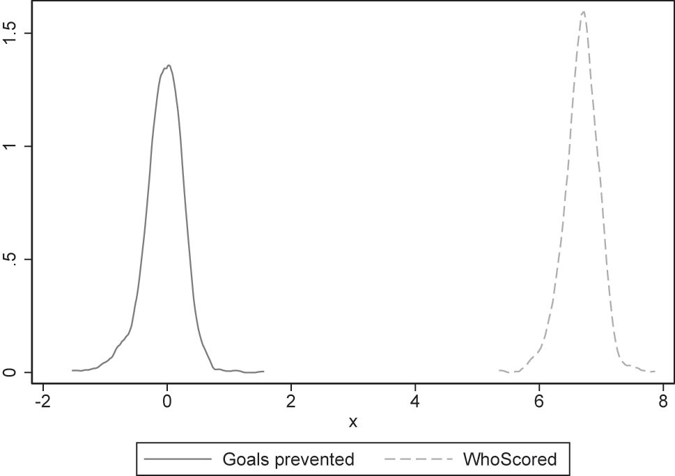
Distribution of goalkeeper performances – Kernel density estimates.
4 Empirical Analysis and Results
The analysis focuses on two types of internal rivalry: implicit rivalry and explicit rivalry. Implicit rivalry includes expected player abilities (proxied by ex ante and adjusted market values) and the age difference between two players – the first accounts for lagged performance and overall player quality and education/training. The latter accounts for the fact that goalkeeper rivals meet at different points in their careers. This is important as it makes a difference whether a veteran player competes against a newcomer or whether there is a rivalry of equals. Furthermore, we consider whether a duo of goalkeepers has already been competing for the number-one status in the previous season or whether there is a new duo constellation. Ultimately, we understand implicit rivalry to illustrate the competitive thread the peer presents at the beginning of an individual period.
Explicit rivalry, on the other hand, refers to concurrent performance on the pitch. By adding explicit rivalry, we strive to observe whether it is demonstrated performance rather than expected performance capability (implicit rivalry) that triggers peer effects. To do so, we need to restrict to goalkeeper duos where both players have the opportunity to play in a given period.
In the first step, we specify a model of goalkeeper performance in professional soccer accounting for implicit internal rivalry and assume that the performance of player i in half-season t competing against peer j in team k is given by.
where dAbility denotes the differences in the expected ability of goalkeeper i and his peer (teammate) j at the beginning of an individual observation period, dAGE is an indicator for the absolute value of the age difference between the players in years and No1 is a dummy variable indicating whether player i can be considered team k’s number one goalkeeper at the beginning of t. We do include some interaction terms to account for asymmetric effects related to status (number one goalkeeper and challenger) and the career situation: firstly, for the difference in abilities considering number one players only (dAbility · No1),[14] and secondly, for the age difference and a dummy indicating whether player i is older than j (dAGE · Older, both also interacted with the No1 indicator). As further controls, the vector X itkj includes league dummies and player i’s age, age squared, and age-adjusted market value as a proxy for ability. Finally, we include team and season fixed effects represented by θ k and Φ t to control for unobserved team characteristics and time trends. Examples of team characteristics we expect to remain stable over our observation period of four years are a club’s (relative) financial means closely related to the (relative) quality of the squad, the general style of play (defensive vs. offensive, formation, etc.) and expectations of fans and management.
Expected player abilities are measured using adjusted transfermarkt market values[15] published before the start of the individual observation period.[16] As scholars have already identified a player’s age and participation in the national team as the most important drivers for market values next to the player’s pure ability or talent,[17] we follow Franck and Nüesch (2012)’s approach and proxy a player’s expected ability by the residuals of a regression of age, age squared and national team participation on market values. This procedure allows us to separate ability from the investment information included in the market value: older players, for instance, show a very low or no high resale value. Furthermore, it reduced the ‘attention bias’ from being selected to the national team.
Implicit rivalry in our setting is based on the initial characteristics of each goalkeeper duo. However, it may be that it is the observable performance that triggers internal competition: players need to prove their quality in official matches. To account for explicit rivalry, we, therefore, add the variable Performance peer to our model defined by (4). Performance peer accounts for the explicit threat of rivalry given the peer’s demonstrated performance in the running period, considering performances in the respective league and the main rounds of either Champions or Europa League.[18] Given the fact that in-season replacements in the goalkeeper position are not a standard, around one-third of observations are linked to the same player without a peer even getting the chance to prove his skills, which leads to a loss of observations when expanding the model for explicit rivalry. The interaction term Performance peer · No1 is included to test whether peer performance affects first-choice goalkeepers and challengers differently, allowing to identify whether an individual player’s standing in the team impacts how peer effects operate.
We perform ordinary least squares (OLS) regressions to estimate our model. Standard errors are clustered at the player-team level.
4.1 Results
Table 4 presents OLS estimates using WhoScored ratings and goals prevented values (GP) to assess goalkeeper performance. Columns (1) and (2) show estimates of model (4), including the implicit threat of the peer only. Columns (3) and (4) also cover the peer’s explicit threat, reducing the sample to observations with substitutions on the goalkeeper position.
Regression results – implicit and explicit rivalry.
| Implicit rivalry | Explicit rivalry | |||
|---|---|---|---|---|
| WhoScored | GP | WhoScored | GP | |
| (1) | (2) | (3) | (4) | |
| Ability differenced | −0.009 (0.016) | −0.008 (0.017) | −0.009 (0.018) | −0.002 (0.021) |
| No1 status | −0.009 (0.027) | −0.056b (0.027) | −0.715b (0.355) | −0.099a (0.036) |
| Age difference | 0.019 (0.017) | 0.030 (0.021) | 0.023 (0.021) | 0.024 (0.026) |
| Older | −0.002 (0.033) | 0.042 (0.037) | −0.011 (0.041) | 0.048 (0.048) |
| Ability difference · No1 | 0.024 (0.019) | 0.006 (0.017) | 0.023 (0.021) | −0.014 (0.020) |
| Age difference · No1 | 0.012 (0.017) | 0.016 (0.019) | 0.018 (0.021) | 0.022 (0.024) |
| Older · No1 | 0.037 (0.037) | 0.087b (0.042) | 0.069 (0.048) | 0.144a (0.054) |
| Age difference · older | −0.039c (0.022) | −0.066a (0.024) | −0.057b (0.028) | −0.067b (0.032) |
| New duo | 0.020 (0.020) | 0.032 (0.024) | 0.025 (0.025) | 0.042 (0.033) |
| Performance peer | −0.130b (0.050) | −0.089b (0.035) | ||
| Performance peer · No1 | 0.100c (0.054) | 0.068 (0.042) | ||
| League dummies | Yes | Yes | Yes | Yes |
| Team FE | Yes | Yes | Yes | Yes |
| Season FE | Yes | Yes | Yes | Yes |
| Observations | 1,292 | 1,272 | 931 | 875 |
| R 2 | 0.188 | 0.210 | 0.240 | 0.248 |
| Mean dep. var. | 6.680 | −0.049 | 6.661 | −0.074 |
-
OLS estimates, a(b/c) indicates significance at the 1 % (5 %/10 %) level. Robust standard errors, clustered at the player-team level, are presented in parentheses. Dependent variable: The focused player’s performance, measured by WhoScored ratings (columns (1) and (3)) and the number of expected goals prevented (columns (2) and (4)). dPlayer ability is proxied by adjusted market values. Further controls include a player’s age, age squared, and adjusted market value, and an indicator variable related to national cup participations of the peer player. Ability and age differences are standardised.
First, we find that a peer’s implicit threat measured in the difference in expected abilities does not significantly impact goalkeeper performance, regardless of the performance indicator used.[19] Instead, we find significant and negative performance effects for the explicit peer threat. In the case of WhoScored ratings, an increase in the peer’s performance by one point on a 10-point scale is associated with a decrease in player i’s performance by 0.13. Since the performance variables are average values over a half-season span with comparatively little dispersion (see Figure 1: 50 % of the observations are between 6.36 and 6.90), this effect is not negligible. However, these findings do not relate to goalkeepers considered a team’s number one in the given season as estimates with and without interaction with a player’s number one status almost balance each other out.[20] In the context of the theoretical framework presented in Section 2, our findings suggest that a performance discouragement effect is present for the underdog but of a smaller magnitude for the favourite. Hence, we conclude that the idea of disappointment aversion presented by March and Sahm (2017) could indeed be a possible reason to explain performance effects in competitive scenarios.
Furthermore, we can document interesting results for the age-related variables included to consider for individual career concerns. First, we find that conditional on his own age, the older player’s performance is negatively correlated with the age gap between him and the rival. This might be explained by the lower long-term ambitions of players who are more advanced in their careers. The effect, however, is substantially smaller than the explicit rivalry effect.
Second, it also shows that the performance of goalkeepers with ‘number one’ status tends to be higher when he is older than his rival. Given the conceptual framework presented in Section 2, a possible explanation is that driven by the ‘fear of losing’, number 1 – goalkeepers may react stronger to younger (and hence ‘hungry’) contenders than to peers at the end of their career. However, since the estimated coefficient of the interaction term Older · No1 has statistical significance only for goals prevented, we take the result with caution.
Finally, we do not find our data to provide convincing evidence on goalkeeper performance being affected by being called out as the team’s number one alone and being attributed to a new opponent.
4.2 Robustness Check: Rotations due to Quasi-Random Shocks
Now that in-season rotations in the goalkeeper position result from proactive team manager decisions, we see the need to address potential endogeneity problems from non-random player selection and reverse causality, i.e. poor focused player performances leading to player substitutions. To do so, we repeat our analysis using sub-samples covering player substitutions caused by injuries and dismissals.[21] We focus on (i) all forced rotations as well as on (ii) forced rotations due to bans and small (moderate) injuries with a maximum duration of 4 (6) match days. The latter is crucially important to check for the robustness of our results and to ensure that long-term injuries potentially impacting a player’s performance capability are excluded.[22]
Table 5 shows the OLS estimates for forced rotations. Generally, our main results on explicit rivalry are robust to quasi-random shocks illustrated by forced rotations. The table illustrates comparable yet stronger performance effects for an explicit peer threat both in size as well as in statistical significance: A one-unit increase in (average) rankings and prevent goals for the peer (teammate) leads to a drop in player i’s performances between 0.31 and 0.43 in WhoScored ratings and between 0.22 and 0.28 in goals prevented values. Again, these findings apply to the underdog in a given duo only as estimates for the coefficient of the interaction term are positive and of roughly equivalent size, leading to our conclusion that effects balance each other out. However, this does not apply for the case of short-term absence rotations only (columns (5) and (6)), which may suggest a discouraging effect even for the number one player. Nevertheless, we are cautious with this interpretation due to the massive loss of observations.
Regression results: forced rotations.
| Bans + | All injuries | Moderate injuriesd | Small injuriese | |||
|---|---|---|---|---|---|---|
| WhoScored | GP | WhoScored | GP | WhoScored | GP | |
| (1) | (2) | (3) | (4) | (5) | (6) | |
| Ability differencef | −0.018 (0.022) | 0.010 (0.027) | −0.006 (0.028) | 0.012 (0.031) | −0.026 (0.032) | 0.002 (0.039) |
| No1 status | −1.464b (0.602) | 0.016 (0.058) | −1.957b (0.777) | 0.003 (0.066) | −1.057 (0.929) | −0.044 (0.083) |
| Age difference | 0.066 (0.041) | −0.002 (0.041) | −0.007 (0.065) | −0.061 (0.058) | −0.039 (0.057) | −0.083 (0.064) |
| Older | −0.055 (0.070) | −0.018 (0.088) | 0.057 (0.103) | 0.149 (0.127) | 0.100 (0.099) | 0.139 (0.155) |
| Ability difference · No1 | 0.020 (0.026) | −0.021 (0.029) | 0.013 (0.027) | −0.008 (0.031) | 0.023 (0.029) | −0.012 (0.033) |
| Age difference · No1 | 0.026 (0.034) | 0.022 (0.038) | 0.027 (0.046) | 0.010 (0.044) | 0.062 (0.043) | 0.051 (0.058) |
| Older · No1 | 0.031 (0.079) | 0.037 (0.079) | −0.087 (0.103) | 0.002 (0.101) | −0.086 (0.109) | 0.029 (0.116) |
| Age difference · older | −0.091c (0.047) | −0.060 (0.048) | −0.028 (0.071) | −0.008 (0.073) | −0.028 (0.061) | −0.022 (0.084) |
| New duo | 0.073 (0.046) | 0.113b (0.051) | 0.053 (0.064) | 0.054 (0.065) | 0.068 (0.084) | 0.097 (0.092) |
| Performance peer | −0.309a (0.077) | −0.218a (0.059) | −0.425a (0.103) | −0.280a (0.078) | −0.385a (0.133) | −0.222b (0.109) |
| Performance peer · No1 | 0.217b (0.090) | 0.142b (0.072) | 0.300b (0.116) | 0.227b (0.095) | 0.160 (0.141) | 0.146 (0.119) |
| League dummies | Yes | Yes | Yes | Yes | Yes | Yes |
| Team FE | Yes | Yes | Yes | Yes | Yes | Yes |
| Season FE | Yes | Yes | Yes | Yes | Yes | Yes |
| Observations | 418 | 421 | 274 | 275 | 207 | 208 |
| R 2 | 0.330 | 0.366 | 0.434 | 0.421 | 0.538 | 0.441 |
| Mean dep. var. | 6.683 | −0.047 | 6.675 | −0.049 | 6.684 | −0.036 |
-
OLS estimates, a(b/c) indicates significance at the 1 % (5 %/10 %) level. Robust standard errors, clustered at the player-team level, are presented in parentheses. Dependent variable: The focused player’s performance, measured by WhoScored ratings (columns (1) and (3)) and the number of expected goals prevented (columns (2) and (4)). dInjury with a duration of less than 7 match days. eInjury with a duration of less than 5 match days. fPlayer ability is proxied by adjusted market values. Further controls include a player’s age, age squared, and adjusted market value and two indicator variables related to the ‘older player status’ (Older) and national cup participations of the peer player. Ability and age differences are standardised.
5 Conclusions
It is often claimed that worker competition is good for business because it increases individual performance. Empirical evidence for an effort-enhancing effect of personal rivalry can, for example, be found in Ager et al. (2022), who document that rivalry motivated by recognition increases effort and risk-taking among German fighter pilots during World War II.
However, there is already a variety of studies using data from professional sports, calling this widely accepted belief into question. This is particularly true for situations where contestants find themselves in battles with heterogeneous abilities and, thus, uneven probabilities of winning. Brown (2011) demonstrates a so-called ‘superstar effect’ in men’s Golf, resulting in poorer results for players once a dominating player (Tiger Woods) participates in a tournament. Focusing on swimmers, Yamane and Hayashi (2015) show that athletes swim faster when chased but slower when their peers are ahead. Lallemand et al. (2008) and Sunde (2003) use data from tennis to show that in uneven contests, ex ante disadvantaged players appear to be less performing while the favourite’s performance outcome tends to improve.
Concentrating on the goalkeeper rivalry in professional soccer, we provide additional evidence that competition impacts performance, but not positively. In line with contest theory, we show that the actual effect of competition on an individual’s performance does crucially depend on an athlete’s standing and status in the team: While the ex ante disadvantaged underdog in a duo of two goalkeepers happens to feel demotivated, thus causing a drop in performance outcomes, we cannot observe the same effect for the ex ante advantaged favourite. Instead, we find the ex ante advantaged player to be rather immune to external influences and not as strongly affected by workplace competition. Ultimately, we conclude that a discouragement effect is present for the underdog but almost absent for the favourite.
However, this effect can only be found in a setting where rivalry works explicitly, meaning that both players get the chance to prove their skills in a given season. Thus, a particularly interesting finding of our analysis is that a competing colleague’s initial set of skills, knowledge and capability does play a minor role in the emergence of peer effects. In contrast, observable performance appears to be the decisive factor. Therefore, we argue that workplace competition generally works explicitly rather than implicitly and that demonstrated performance outweighs pure skills.
Adding to these findings on actual performance-on-performance effects, we see that the difference in age between two contestants also impacts on-pitch performance. Our data support the conclusion that the age gap is negatively associated with the older player’s performance but that the performance of goalkeepers with ‘number one’ status is higher in the face of a younger contender. We explain these findings with age-related differences in long-term career ambitions.
With existing studies widely focusing on anonymous face-to-face competitions between individuals not socially tied to each other, we show that rivalry might as well impact individual performance even when peers are not directly competing and thus support Pike et al. (2018, p. 805) in suggesting that “rivalry has a long motivational shadow”. Furthermore, we show that performance-affecting competition does not only exist between teams with opposing outcomes but within teams as well, thus emphasising the relational aspect of rivalry.
Our findings contribute to existing studies on peer effects in workplace situations as follows: While performance-related peer effects among colleagues are widely explained by the concept of productivity spillovers or – in case of negative performance effects – free-riding, we present in-team rivalry as a different mechanism to explain changes in co-workers’ productivity. The inherent characteristic of workplace rivalry is that employees do not fight for career advancement in isolation. Instead, with in-house career opportunities being a limited resource, they find themselves indirectly competing against colleagues.
Our conclusions may be especially beneficial for managers as we take the result of a labour market sorting as a given, allowing us to rate management decisions on team/partner formation. Ultimately, our findings indicate that internal competition may have an adverse effect on output in the case of heterogeneity in abilities and career stages. We recommend considering these worker characteristics for the design of internal workplace competition.
Acknowledgments
We would like to thank Houda Ben Said and Julian Herwig for their excellent assistance in preparing the data. We are also grateful to W. David Allen, Joachim Grosser, Michael Möcker, and participants of the ESEA meeting in 2021 for their helpful comments.
References
Ager, P., L. Bursztyn, L. Leucht, and H.-J. Voth. 2022. “Killer Incentives: Rivalry, Performance and Risk-Taking Among German Fighter Pilots, 1939–45.” The Review of Economic Studies 89 (5): 2257–92. https://doi.org/10.1093/restud/rdab085.Search in Google Scholar
Allen, W. D. 2021. “Work Environment and Worker Performance: A View from the Goal Crease.” Journal of Labor Research 42 (3): 418–48. https://doi.org/10.1007/s12122-021-09323-w.Search in Google Scholar
Baik, K. H. 1994. “Effort Levels in Contests with Two Asymmetric Players.” Southern Economic Journal 61 (2): 367–78. https://doi.org/10.2307/1059984.Search in Google Scholar
Bandiera, O., I. Barankay, and I. Rasul. 2010. “Social Incentives in the Workplace.” The Review of Economic Studies 77 (2): 417–58. https://doi.org/10.1111/j.1467-937x.2009.00574.x.Search in Google Scholar
Brown, J. 2011. “Quitters Never Win: The (Adverse) Incentive Effects of Competing with Superstars.” Journal of Political Economy 119 (5): 982–1013. https://doi.org/10.1086/663306.Search in Google Scholar
Bryson, A., B. Frick, and R. Simmons. 2013. “The Returns to Scarce Talent: Footedness and Player Remuneration in European Soccer.” Journal of Sports Economics 14 (6): 606–28. https://doi.org/10.1177/1527002511435118.Search in Google Scholar
Buchanan, J. M., R. D. Tollison, and G. Tullock. 1980. Toward a Theory of the Rent Seeking Society. College Station: Texas A&M Press.Search in Google Scholar
Dendir, S. 2016. “When Do Soccer Players Peak? A Note.” Journal of Sports Analytics 2 (2): 89–105. https://doi.org/10.3233/jsa-160021.Search in Google Scholar
Franck, E., and S. Nüesch. 2012. “Talent And/or Popularity: what Does it Take to Be a Superstar?” Economic Inquiry 50 (1): 202–16. https://doi.org/10.1111/j.1465-7295.2010.00360.x.Search in Google Scholar
Gauriot, R., and L. Page. 2019. “Fooled by Performance Randomness: Overrewarding Luck.” The Review of Economics and Statistics 101 (4): 658–66. https://doi.org/10.1162/rest_a_00783.Search in Google Scholar
Gerhards, J., and M. Mutz. 2017. “Who Wins the Championship? Market Value and Team Composition as Predictors of Success in the Top European Football Leagues.” European Societies 19 (3): 223–42. https://doi.org/10.1080/14616696.2016.1268704.Search in Google Scholar
Gould, E. D., and E. Winter. 2009. “Interactions between Workers and the Technology of Production: Evidence from Professional Baseball.” The Review of Economics and Statistics 91 (1): 188–200. https://doi.org/10.1162/rest.91.1.188.Search in Google Scholar
Guryan, J., K. Kroft, and M. J. Notowidigdo. 2009. “Peer Effects in the Workplace: Evidence from Random Groupings in Professional Golf Tournaments.” American Economic Journal: Applied Economics 1 (4): 34–68. https://doi.org/10.1257/app.1.4.34.Search in Google Scholar
He, M., R. Cachucho, and A. J. Knobbe. 2015. “Football Player’s Performance and Market Value.” In Proceedings of the 2nd Workshop of Sports Analytics, European Conference on Machine Learning and Principles and Practice of Knowledge Discovery in Databases (ECML PKDD). Also available at: http://ceur-ws.org/Vol-1970/paper-11.pdf.Search in Google Scholar
Herbst, D., and A. Mas. 2015. “Peer Effects on Worker Output in the Laboratory Generalize to the Field.” Science 350 (6260): 545–9. https://doi.org/10.1126/science.aac9555.Search in Google Scholar
Kahn, L. M. 2000. “The Sports Business as a Labor Market Laboratory.” The Journal of Economic Perspectives 14 (3): 75–94. https://doi.org/10.1257/jep.14.3.75.Search in Google Scholar
Kalén, A., E. Rey, A. S. de Rellán-Guerra, and C. Lago-Peñas. 2019. “Are Soccer Players Older Now Than before? Aging Trends and Market Value in the Last Three Decades of the UEFA Champions League.” Frontiers in Psychology 10: 76. https://doi.org/10.3389/fpsyg.2019.00076.Search in Google Scholar
Kandel, E., and E. P. Lazear. 1992. “Peer Pressure and Partnerships.” Journal of Political Economy 100 (4): 801–17. https://doi.org/10.1086/261840.Search in Google Scholar
Konrad, K. 2009. Strategy and Dynamics in Contests. LSE Perspectives in Economic Analysis. Oxford: Oxford University Press.Search in Google Scholar
Lackner, M., and H. Sonnabend. 2023. “Presenteeism when Employers Are under Pressure: Evidence from a High-Stakes Environment.” Economica 90 (358): 477–507. https://doi.org/10.1111/ecca.12461.Search in Google Scholar
Lallemand, T., R. Plasman, and F. Rycx. 2008. “Women and Competition in Elimination Tournaments: Evidence from Professional Tennis Data.” Journal of Sports Economics 9 (1): 3–19. https://doi.org/10.1177/1527002506296552.Search in Google Scholar
March, C., and M. Sahm. 2017. “Asymmetric Discouragement in Asymmetric Contests.” Economics Letters 151: 23–7. https://doi.org/10.1016/j.econlet.2016.11.032.Search in Google Scholar
Mas, A., and E. Moretti. 2009. “Peers at Work.” The American Economic Review 99 (1): 112–45. https://doi.org/10.1257/aer.99.1.112.Search in Google Scholar
Mobbs, S., and C. G. Raheja. 2012. “Internal Managerial Promotions: Insider Incentives and CEO Succession.” Journal of Corporate Finance 18 (5): 1337–53. https://doi.org/10.1016/j.jcorpfin.2012.09.001.Search in Google Scholar
Müller, O., A. Simons, and M. Weinmann. 2017. “Beyond Crowd Judgments: Data-Driven Estimation of Market Value in Association Football.” European Journal of Operational Research 263 (2): 611–24. https://doi.org/10.1016/j.ejor.2017.05.005.Search in Google Scholar
Pike, B. E., G. J. Kilduff, and A. D. Galinsky. 2018. “The Long Shadow of Rivalry: Rivalry Motivates Performance Today and Tomorrow.” Psychological Science 29 (5): 804–13. https://doi.org/10.1177/0956797617744796.Search in Google Scholar
Pitts, J. D., and B. Evans. 2019. “Manager Impacts on Worker Performance in American Football: Do Offensive Coordinators Impact Quarterback Performance in the National Football League?” Managerial and Decision Economics 40 (1): 105–18. https://doi.org/10.1002/mde.2985.Search in Google Scholar
Serna Rodríguez, M., A. Ramírez Hassan, and A. Coad. 2019. “Uncovering Value Drivers of High Performance Soccer Players.” Journal of Sports Economics 20 (6): 819–49. https://doi.org/10.1177/1527002518808344.Search in Google Scholar
Sonnabend, H. 2020. “On Discouraging Environments in Team Contests: Evidence from Top-Level Beach Volleyball.” Managerial and Decision Economics 41 (6): 986–97. https://doi.org/10.1002/mde.3153.Search in Google Scholar
Sunde, U. 2003. Potential, Prizes and Performance: Testing Tournament Theory with Professional Tennis Data. IZA Discussion Paper no. 947.10.2139/ssrn.477442Search in Google Scholar
Sunde, U. 2009. “Heterogeneity and Performance in Tournaments: a Test for Incentive Effects Using Professional Tennis Data.” Applied Economics 41 (25): 3199–208. https://doi.org/10.1080/00036840802243789.Search in Google Scholar
Yamane, S., and R. Hayashi. 2015. “Peer Effects Among Swimmers.” The Scandinavian Journal of Economics 117 (4): 1230–55. https://doi.org/10.1111/sjoe.12124.Search in Google Scholar
© 2024 the author(s), published by De Gruyter, Berlin/Boston
This work is licensed under the Creative Commons Attribution 4.0 International License.
Articles in the same Issue
- Frontmatter
- Editorial
- Guest Editorial
- Special Issue Articles
- Is Blood Thicker than Water? The Impact of Player Agencies on Player Salaries: Empirical Evidence from Five European Football Leagues
- When Colleagues Come to See Each Other as Rivals: Does Internal Competition Affect Workplace Performance?
- Pregnancy in the Paint and the Pitch: Does Giving Birth Impact Performance?
- An Empirical Estimation of NCAA Head Football Coaches Contract Duration
- Race, Market Size, Segregation and Subsequent Opportunities for Former NFL Head Coaches
- Football Fans’ Interest in and Willingness-To-Pay for Sustainable Merchandise Products
- Change in Home Bias Due to Ghost Games in the NFL
- Consumer Perceptions Matter: A Case Study of an Anomaly in English Football
- Talent Allocation in European Football Leagues: Why Competitive Imbalance May be optimal?
- Data Observer
- SOEP-LEE2: Linking Surveys on Employees to Employers in Germany
- The IAB-SMART-Mobility Module: An Innovative Research Dataset with Mobility Indicators Based on Raw Geodata
- Miscellaneous
- Annual Reviewer Acknowledgement