
Spatio-temporal trajectory alignment for trajectory evaluation
-
Gereon Tombrink

 ,
Ansgar Dreier
,
Ansgar Dreier

Abstract
Assessing the quality of a trajectory is a prerequisite for correctly interpreting and using the trajectory in applications such as kinematic laser scanning. Evaluation is for example done empirically by comparison with a ground-truth trajectory recorded simultaneously. Depending on the measurement and sensor configuration, both trajectories have to be aligned before comparison. Usually, either a similarity transformation or a rigid-body transformation is used for this purpose. We propose an extended spatio-temporal alignment, which additionally supports the estimation of a lever arm and a time offset between both trajectories. Our method can be used to align two trajectories of the same vehicle captured simultaneously by different sensors. We apply the approach on several recorded data sets and evaluate it empirically. We show that although real-world data sets can lead to high correlations between parameters, they can still be successfully aligned and evaluated using the methodology. To enable replication of our research, we publish the code which is available here: https://github.com/gereon-t/trajectopy.
1 Introduction
Estimating the position and the orientation of a vehicle over time, i.e. its trajectory, is a crucial component in many applications such as autonomous driving, public transport or kinematic laser scanning [1], [2], [3]. Besides the estimation itself, the ability to provide an uncertainty of the estimated position and orientation (pose) is often equally important, especially in safety-critical domains, e.g. in deformation monitoring. A realistic understanding of the trajectory accuracy helps in the interpretation and processing of the determined poses. The derivation of such an uncertainty is often done empirically by comparing the estimated trajectory to a ground-truth trajectory generated using sensors or knowledge of higher accuracy [4], [5], [6], [7].
Depending on the sensors used for trajectory estimation, both trajectories may need to be aligned before comparison [8]. For example, the ground truth trajectory might be given in a global reference frame while the estimated trajectory consists of poses defined in some arbitrary local frame. Furthermore, due to different mounting positions on the vehicle, a lever arm might exist between the two systems. Finally, it may not be possible to fully synchronize both sensors to a common time reference, resulting in residual synchronization errors.
The usual approach to this trajectory alignment problem is to estimate a similarity or rigid body transformation between the two trajectories to compensate for any differences in the coordinate systems. The closed-form methods by [9], 10] using a singular value decomposition of the covariance matrix of the position data have become particularly popular for this purpose [8]. However, to the best of our knowledge, there are no alignment approaches also considering a lever arm and a time shift between both trajectories. Lever arms are typically either measured or derived from construction blueprints [4], [11], [12], [13], [14]. If both systems are on the same vehicle, synchronization deviations can often be avoided using triggered measurements logged in a central time reference, such as an inertial measurement unit (IMU) or an onboard computer [13]. In summary, the alignment of the coordinate systems is therefore mostly solved mathematically, while the lever arm and the synchronization are taken into account by suitable methods before and during the measurement.
However, there are situations where the lever arm and the synchronization between two navigation sensors cannot be fully controlled. The lever arm could be unknown or not measurable, because the position of the reference points of the sensors are unknown or physically inaccessible. Furthermore, measurements of some sensors cannot be triggered or referenced to the same time frame, resulting in time delays. For example, this is usually the case when global time systems such as GPS time are used in conjunction with local computer times. A GPS time-based reference trajectory using non-triggerable total stations is presented in [15], but this publication is limited to synchronization without comprehensive alignment including similarity transformation and lever arm.
Therefore, we propose a method to align the positions of two simultaneously recorded trajectories of the same vehicle in both spatial and temporal domains. This spatio-temporal alignment supports a similarity transformation, a lever arm transformation, and a time offset. After aligning the test trajectory with a recorded ground truth trajectory, the precision of the test trajectory can be evaluated using pose-wise comparisons. Since the alignment process corrects for constant systematic deviations of both trajectories, it is not possible to make a thorough statement about the accuracy of the test trajectory. However, once the alignment has been determined, the change in these systematic deviations and the reproducibility of the trajectory estimate can be examined, which provide valuable information about the quality.
The second contribution is the empirical evaluation of the methodology using different datasets. For this purpose, we apply the method to recorded trajectories of different speeds and shapes using a GNSS/IMU system and a total station. The focus of the study is on the quality of the parameter estimation in terms of correlation and stability and on the suitability of the spatio-temporal alignment for trajectory comparisons. Although not covered in this paper, the methodology presented is not only suitable for the evaluation but also for the combination of different sensors. Once two sensors have been successfully aligned, the calibration parameters required for a combination are known.
The remainder of the paper is structured as follows. In the subsequent Section 2, the methodology of the spatio-temporal alignment is described. This is followed in Section 3 by the acquisition of measurement data in the context of various experiments. Finally, the results of the experiments are presented and discussed in Section 4.
2 Methodology
The overarching goal is the comparison of two trajectories, a reference trajectory of superior accuracy and an estimated test trajectory from a system under test. However, for various reasons, it may be necessary to align both trajectories before comparison. The general procedure of the trajectory evaluation is shown in Figure 1, with the alignment step colored in blue. Without going into further detail, we assess the precision of the test trajectory after alignment using along- and cross-track deviations as shown in [7] (see Figure 1, yellow). Our paper focuses on the spatio-temporal alignment, which is explained in the following sections.
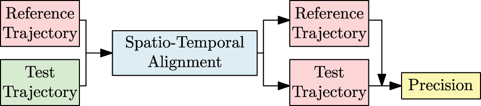
General procedure of the trajectory evaluation. The reference and test trajectories are initially separated by a spatio-temporal transformation. After alignment, the test trajectory can be compared with the reference to determine its precision.
A trajectory T describes the positions p(k) and the orientations o(k) of a vehicle at N discrete points in time k, i.e.:
Each pair of a position and an orientation form a pose. We assume that both the positions and the orientations refer to the same world coordinate system. We denote the world frame of the reference by r and that of the estimated test trajectory by e. In addition to these two coordinate systems, the sensor frame s of the aligned navigation sensor is also relevant for the further methodology. Note that, unlike with the world coordinate systems (r and e), we do not distinguish between two individual s-frames here, as we assume that the axes of both s-frames are already aligned and that there is only a translation between them. The origin of the s-frame is usually located inside the navigation sensor while the axis directions depend on the configuration and mounting of the particular system, but are usually aligned with the direction of travel of the vehicle. Figure 2 shows both types of frames, world frame w and sensor frame s.
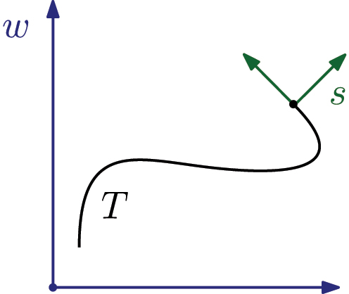
Relevant coordinates systems: w-frame and s-frame, here shown in 2D.
2.1 Problem formulation
We would like to compare two trajectories, an estimated trajectory T e and a reference trajectory T r that describe the movement of the same vehicle at the same time. We assume that both trajectories are sampled at the same time stamps, establishing a direct pose correspondence. This can be achieved, for example, by interpolation or by appropriate actions during the measurement. Note that identical timestamps of two trajectories do not necessarily mean that they are synchronized. If the time references of both trajectories are shifted, e.g. due to limitations of the sensors used, the matching process will rely on incorrect time stamps, resulting in synchronization errors. Furthermore, both trajectories may be defined in different world coordinate systems and have differently located sensor origins.
We aim to describe these differences using the positions of both trajectories. Therefore, the goal of the methodology is to estimate all unknown parameters of a transformation g, so that
with
First, the positions p
e
(k) are shifted by the three-dimensional lever arm
Due to our simplifying assumptions regarding the coordinate systems (see Section 2), we can also align o
e
(k) to (o
e
(k))′ using
In total there are up to 11 parameters
Depending on the sensors used and the measurement setup, some of those parameters may already be known.
2.2 Least squares adjustment
We estimate any unknown transformation parameters within an iterative least squares adjustment using N epochs of observations. The observations actually required for alignment depend on the parameters to be estimated. In any case, the positions of both trajectories are necessary. To estimate the lever arm, the orientation of the vehicle on which both sensors are mounted is also required. For estimating the time offset, the three-dimensional velocity of the vehicle must be available. The orientation and the velocity information can be provided by the sensors used or, to further decouple the alignment from the sensors under investigation, by third independent sensors.
Assuming full parameter estimation, the observation vector consists of the individual components of the trajectory positions, the vehicle orientation, and the vehicle velocity, for all time stamps k = 1, …, N:
The observations can be introduced to the parameter estimation process with appropriate a-priori variances.
The least-squares adjustment requires a mathematical model h(l k , x), also called functional model, that relates the recorded observations l k to the unknown parameters x. In our case, the functional model is
Since we usually have a large number of observation epochs, we obtain an overdetermined system of equations. Due to measurement deviations, usually h(l k , x) ≠ 0, requiring adjustment theory for optimal parameter estimation. Given the implicit nature of the functional model, we use the Gauss–Helmert–Model to obtain the alignment parameters. We refer to the literature for a comprehensive explanation of the parameter and variance estimation process, as we follow the standard textbook procedure [16], [17], [18].
The fast and successful convergence of the parameter estimation primarily depends on the quality of their initial values x0. Therefore, we first compute an initial similarity transformation using the method described in [10]. After that, we separately compute initial values for both the lever arm and the time shift. Based on the pre-aligned trajectory, the final spatio-temporal alignment is performed within a single adjustment considering all parameters.
After the adjustment, we verify the consistency of the functional and the stochastic model using a stochastic global test. In addition, we divide the observations into groups of similar stochastic properties. Thus, the horizontal position components, the vertical position components, the roll and pitch angle, the yaw angle, and the velocity each form an observation group that can be tested separately.
2.3 Limitations
The methodology presented has several limitations that should not go unmentioned. The orientations are currently not part of the functional model and can only be aligned if their alignment parameters can be inferred from the position alignment. This is only the case if there is no rotation between the s-frames of both sensors and if the positions and the orientations of each trajectory refer to the same w-frame. As soon as there are different orientations of the two sensor systems, this can so far only be taken into account manually, e.g. by calculating the mean rotation difference. Further limitations of the methodology concern the estimability of the individual parameters and the scope of the quality analysis that is possible after the alignment.
The successful estimation of all required alignment parameters strongly depends on the shape and properties of the trajectory. For example, trajectories along a straight line or along a circle would be disadvantageous for determining all three rotation angles of the similarity transformation. Furthermore, there must be a variation in velocity so that v
e
(k)Δt (see Eq. (3)) does not simply become a constant offset that cannot be separated from the lever arm. However, it should also be noted that Eq. (3) assumes a single velocity v
e
(k) for a time interval of length Δt. If this assumption is violated, it adversely affects the estimation process. For instance, with a Δt of 10 ms, the assumed velocity must match the true velocity within 0.1 m/s, ensuring that the resulting deviation is below or equal to one mm. If the time offset is large compared to the speed variations and cannot be prevented otherwise, it is recommended to perform the entire adjustment iteratively and update the matching of both trajectories between iterations. Additionally, it may be reasonable to also consider the acceleration of the vehicle. Regarding the lever arm estimation, it is necessary that the vehicle orientation changes sufficiently over the course of the trajectory. A constant orientation
Another limitation concerns the quality analysis after successful alignment. As the alignment inherently aims to correct systematic deviations between the two trajectories, these can no longer be detected during a subsequent evaluation. For instance, a constant systematic positioning deviation relative to the vehicle may remain unnoticed, as it would be incorporated into the lever arm. On the other hand, with regard to many application areas of mobile mapping systems, the change of systematic deviations is much more critical than the mere existence. A constant systematic deviation that can be completely absorbed by the alignment process may not be relevant, depending on the application. If, for example, a building is captured for deformation monitoring in two epochs, both are equally systematically influenced, which is irrelevant for deciding whether there was a deformation of the object. However, if the systematic deviations of a system change in an unknown way, its suitability for many applications suffers considerably. With regard to the deformation analysis, a deformation can then no longer be distinguished from a systematic deviation. However, such changes can be detected using the methodology described. Once the alignment parameters have been determined, they can be applied to different measurements at different times and under different conditions and checked for consistency.
3 Experiments
In order to investigate the practicability of the proposed method, we conducted experiments using two sensor systems. The systems are a GNSS/IMU system and a total station in kinematic mode, two common sensor systems for pose or position measurements. The measurement conditions resemble typical experimental conditions as they appear in the trajectory estimation of people or vehicles. We performed the experiments to investigate if the method is able to estimate the necessary parameters to align one system with the other. We also aim to investigate if the requirements in Section 2.3 are easily met and how reproducible and stable the alignment is.
3.1 Test system
Within our studies, we use the real time extended Kalman filter (EKF) solution of the Ellipse2-D from SBG-Systems, which is an inertial navigation system (INS) consisting of a three-axis inertial measurement unit (IMU) and a Global Navigation Satellite System (GNSS) receiver with dual antenna support. We deliberately used the real-time solution provided by the manufacturer and avoided a post-processing trajectory estimation in order to investigate if the proposed alignment is able to determine all necessary parameters within realistic conditions. With an active RTK-link (Real Time Kinematic) and under good GNSS conditions, the data sheet specifies the horizontal positioning accuracy with 2 cm and the vertical positioning accuracy with 4 cm. Orientations follow the Tait-Byran convention and are provided with an accuracy of 0.1° for the roll and pitch angles, while the yaw angle has an accuracy of 0.2°. The velocity of the system is derived with an accuracy 0.03 m/s. We operate the system with two Leica AS10 GNSS antennas. The orientations of the IMU follow the North-East-Down (NED) convention, so the z-axis of its s-frame points downwards.
3.2 Reference system
During all measurements we generate the reference trajectory with a Leica TS60 total station that automatically tracks a 360° prism. Total stations are a good example in terms of spatio-temporal alignment. Due to the nature of their operation, there is a lever arm between the tracked prism and the system being evaluated. In addition, a time offset between the total station and the system under test is usually unavoidable given its internal measurement methodology [19]. Furthermore, depending on the environment of the total station, georeferencing may not be available.
In kinematic mode, the total station has a distance accuracy of 3 mm + 1 ppm according to the manufacturer’s data sheet. Angle measurement is performed with an accuracy of 0.15 mgon, while the accuracy of the tracked prism is specified as 2 mm. Overall, we assume an accuracy of 4 mm for the positions determined by the total station. We consider a total station to be a suitable reference sensor, especially for GNSS-based systems, mainly because these accuracies can be achieved very reliably and independently of the environment.
We use a GPS-capable logging device to control the total station via the Leica GeoCOM protocol and to record its measurements. Incoming messages from the total station can thus be acquired in GPS time, similar to the tested systems. However, there is a time offset between the receipt of the message and the actual time of measurement. In addition to the obvious transmission time, this is mainly due to the way total stations carry out measurements. Several independent subsystems within the instrument are involved during operation, resulting in the inability to precisely trigger a single measurement [19]. Thus, while GPS-based acquisition of the incoming total station messages is highly beneficial for initial synchronization, a final adjustment of the residual time offset is necessary, which we aim to provide with our proposed method.
3.3 Measurement campaigns
In total, two measurement campaigns were conducted using the described sensors:
Hand-held measurement: Short measurement of an arbitrary trajectory with both sensors, which requires the estimation of all alignment parameters except the scale. This experiment is intended to investigate the feasibility of estimating the spatio-temporal alignment parameters with a short low-effort calibration measurement.
Repeated rail-bound measurement: The availability of georeferenced total station data allows this campaign to focus on estimating the time offset and the lever arm. Furthermore, this campaign was divided into a short-term and a long-term measurement. The first helps to determine all necessary alignment parameters, the second enables us to investigate the long-term stability of the parameters.
The spatial relationship of the GNSS/IMU system and the 360° prism was not changed between both measurement campaigns, so we can assume it is the same. The following sections will describe the individual measurements in detail.
3.3.1 Hand-held measurement
The hand-held measurement took place on the campus of the University of Bonn. The total station (see Figure 3(b)) was placed at an arbitrarily chosen location, horizontally leveled, but not georeferenced. The GNSS/IMU system (see Figure 3(c)) was moved by hand in the vicinity of the total station for approximately 3 min. The GNSS provided new positions at a rate of 5 Hz while the IMU measured at 100 Hz. Care was taken to vary the orientation and speed of the vehicle to meet the requirements mentioned in Section 2.3. The system was tilted, and variations of the roll and pitch angles from about −35° to +35° were obtained. The average speed was 1.1 m/s, with a maximum of about 3.4 m/s. Figure 3(a) shows both trajectories in their unrelated coordinates systems. The total of 17,581 100 Hz EKF positions of the GNSS/IMU system were transformed to a local coordinate system tangent to the GRS80 ellipsoid and oriented to the north. In a second step, they were interpolated onto the 1,249 positions of the tracked 360° prism. These are provided by the total station with an average data rate of 5.9 Hz and are given in a local coordinate system, which is tangent to the geoid due to the leveling of the instrument. The prism was firmly attached to the GNSS/IMU system housing between both GNSS antennas (see Figure 3(c)).
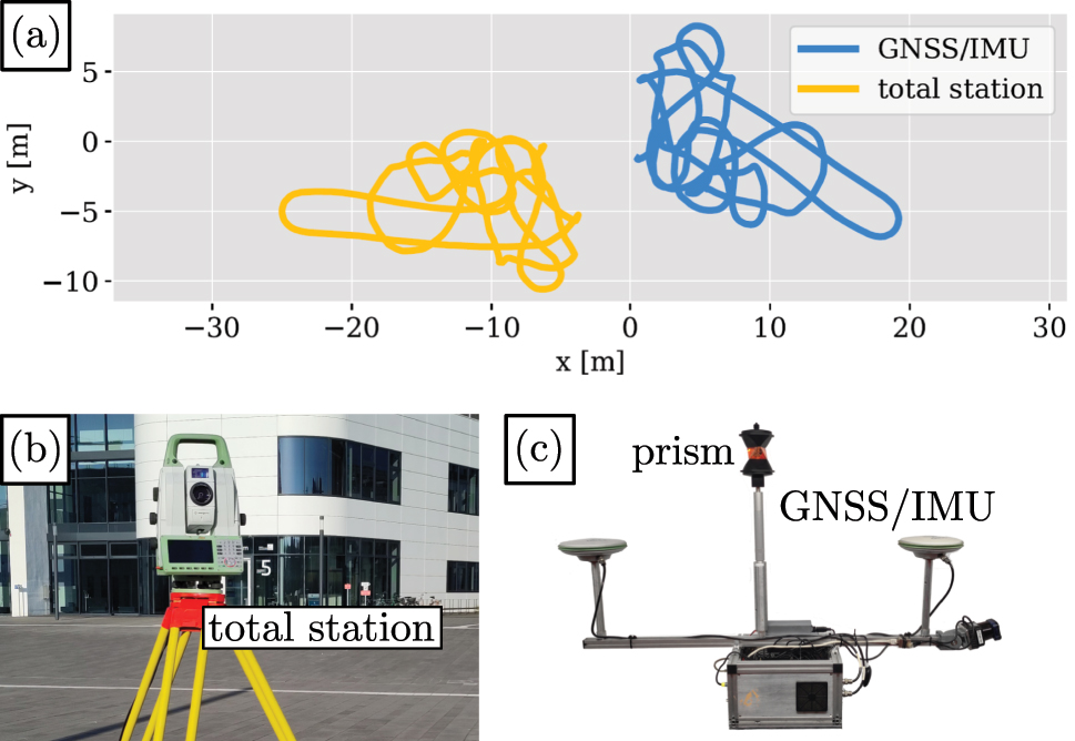
Hand-held measurement on the campus of the University of Bonn. (a) Ground track of both recorded trajectories. (b) Leica TS60 total station. (c) GNSS/IMU inertial navigation system from SBG-Systems.
3.3.2 Repeated rail-bound measurement
For the repeated rail-bound measurement we used a rail track (see Figure 4(a)), which is part of a test environment at the University of Bonn. The approximately 140 m long closed-loop track has variations in all degrees of freedom (DOF; three for position, three for orientation) and allows us to repeat the trajectory precisely. For the measurement, the GNSS/IMU system and the 360° prism were mounted on a rail car, displayed in Figure 4(c). The s-frame of the IMU was aligned with the direction of travel, i.e. the x-axis is pointing in the direction of travel, the y-axis to the right and the z-axis downwards. The total station was placed on one of multiple geodetic measurement pillars with known ETRS89 coordinates in close proximity to the track (see Figure 4(b)). Therefore, we were able to georeference the total station using two pillars, leaving only the lever arm and time offset for least-squares estimation.
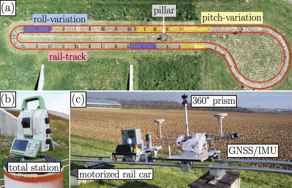
Measurement setup of the rail-bound measurement. (a) Aerial view of the rail-track. (b) Total station used for tracking placed on a pillar within the rail-track. (c) GNSS/IMU system and the 360° prism mounted on the rail car.
The measurement was divided into two parts. In the first part, the rail car was moved manually over the track without motorization. This allowed us to vary the speed, which is essential for the separation of lever arm and time offset (see Section 2.3). During the seven-minute measurement, a maximum speed of 5.5 m/s was reached with an average speed of 1.1 m/s. The data rate of the total station was 6.2 Hz on average, resulting in 2,658 measured prism positions. The GNSS/IMU system was configured to record raw GNSS positions at 5 Hz and IMU data at 50 Hz. The output EKF solution was also set to 50 Hz.
For a second measurement, which lasted 30 min, we used a motorized rail car to automatically move the sensors repeatedly along the track with a speed of approx. 0.75 m/s. This measurement resulted in 91,184 GNSS/IMU poses and 13,545 prism positions and is used to investigate the long-term stability of the alignment parameters.
4 Results and discussion
This section presents and discusses the results of the experiments using the proposed methodology. For both the handheld and the rail-bound measurements, the goal is to align the positions of the GNSS/IMU with the reference positions of the total station. This requires knowledge about the orientation and velocity of the vehicle, which we obtain from the GNSS/IMU system under test. Depending on the measurement configuration, different parameters are unknown and therefore estimated. The observations required in each case are included in the adjustment with uncertainties corresponding to the manufacturer’s specifications (see Section 3). These variances are used to determine the a-posteriori variances of the estimated parameters.
4.1 Hand-held estimation results
Table 1 shows the estimated parameters of the hand-held measurement together with their a-posteriori variances. Due to the arbitrary positioning of the total station, all parameters except the scale are of interest. The determined translation of the similarity transformation reflects the difference between the origin of the two local coordinate systems. Since the trajectory of the GNSS/IMU system was transformed into a local system before alignment, the values are comparatively small. As expected, the rotation around x and y are also very small and not significantly different from zero with respect to the corresponding standard deviations. Apart from measurement deviations, the two angles describe the plumb deviation between the two coordinate systems, which is negligible for our application. Therefore, we also performed the alignment without estimating the two angles. The results of the other parameters remain almost unchanged and are therefore not explicitly listed again. Unlike the rotation around x and y, the rotation around z is very relevant, especially when using total stations. Since we have not determined the orientation of the instrument using known control points, the estimated angle corresponds to the unknown orientation of the total station. The time offset between the total station time and the GPS time due to the challenges described in Section 3 was determined to be −90.3 ms. As expected, the negative value indicates that the measurements of the total station are recorded with a time delay.
Parameter estimation results of the hand-held measurement.
| Parameter | Value | Std. |
|---|---|---|
| Translation x | −10.095 m | 0.8 mm |
| Translation y | −3.788 m | 0.7 mm |
| Translation z | −0.908 m | 2.3 mm |
| Rotation x | 0.099° | 0.021° |
| Rotation y | −0.019° | 0.020° |
| Rotation z | −151.162° | 0.007° |
| Time shift | −90.3 ms | 0.5 ms |
| Lever arm x | 0.016 m | 0.7 mm |
| Lever arm y | 0.002 m | 0.8 mm |
| Lever arm z | −0.695 m | 2.1 mm |
Due to the mounting of the 360° prism with respect to the GNSS/IMU system, there is primarily a lever arm in the z-component, which is confirmed by the determined parameters for the lever arm components. The z-value is negative due to the NED definition of the s-frame of the IMU (see Section 3). Figure 4(c) shows the 360° prism placed along an axis between the two GNSS antennas. The origin of the GNSS/IMU system is located in the IMU, which is centered in the housing below the prism.
Using the determined parameters, the GNSS/IMU trajectory can be aligned to the total station trajectory (see Figure 5). Based on the spatio-temporal alignment of both trajectories, further investigations, such as the comparison of the positions shown in Section 4.5, can be performed.
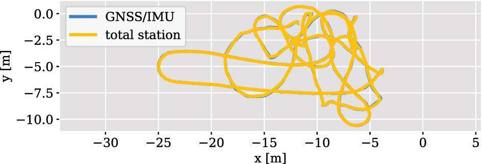
Aligned trajectories of the hand-held measurement.
4.2 Rail-track estimation results
We estimated the alignment parameters for both conducted rail-track measurements. Since the total station has been georeferenced, only the estimation of the time shift and the lever arm parameters is necessary. The first measurement was carried out manually and is characterized by large velocity variations. Therefore, it is used to estimate the lever arm and the time offset between the total station and the GNSS/IMU system. The results of this adjustment are shown in Table 2 (left).
Parameter estimation results of the rail-track measurement.
| Manual | Motorized | |||
|---|---|---|---|---|
| Parameter | Value | Std. | Value | Std. |
| Time shift | −96.8 ms | 0.3 ms | – | – |
| Lever arm x | 0.024 m | 0.5 mm | 0.028 m | 0.2 mm |
| Lever arm y | −0.001 m | 0.4 mm | 0.001 m | 0.2 mm |
| Lever arm z | −0.694 m | 0.8 mm | −0.679 m | 0.3 mm |
For the motorized second measurement, we applied the time offset of −96.8 ms to the total station measurements. This leaves only the lever arm as an unknown for aligning the trajectories from the motorized measurement. Due to the lack of variation in vehicle speed, simultaneous estimation of the lever arm and the time offset would not be possible (see Section 2.3). The determined components of the lever arm are listed in Table 2 (right).
It is noticeable that the common parameters of all three adjustments differ from each other more than the corresponding standard deviation would suggest. The difference between the time offset of the handheld measurement and the time offset of the rail-track measurement is 6.5 ms. Compared to the respective a-posteriori standard deviations of 0.5 ms and 0.3 ms, this is a significant deviation. During the rail measurement, the x-axis of the IMU s-frame was always oriented in the direction of travel. Thus, the x-component of the lever arm and the time offset have a very similar influence on the alignment result. At the average velocity of 1.06 m/s, the observed difference of 6.5 ms corresponds to 6.9 mm. This is similar to the difference in the lever arm x-component of both measurements of about 8 mm. Due to the always identical orientation of the system relative to the direction of travel, it is possible that the lever arm and the time offset cannot be sufficiently separated from each other, resulting in the parameter estimation differences. This explanation is backed up by the correlation analysis in Section 4.4.
Another noticeable observation is that the lever arm z-components differ by 1.5 cm between the two rail track measurements. One reason for this could be systematic deviations in GNSS positioning. Since the alignment is performed based on the sensor observations, any deviations directly affect the result of the estimation.
The determined a-posteriori variances are consistently very small. There are two main reasons for this. First, for lack of alternatives, we assume that all observations of the alignment are uncorrelated. In most cases, this assumption is a simplification of the actual stochastics. On the other hand, there is a large number of observations, which is contrasted with a comparatively small number of parameters. This very high redundancy combined with uncorrelated observations leads to small estimates of the a-posteriori variances, which are often too optimistic, especially with respect to systematic deviations. To support this hypothesis, we investigate the temporal variation of the estimated lever arm in the following section.
4.3 Parameter stability
In this subsection, the time stability of the lever arm estimate is examined using the motorized rail-track measurement. For this purpose, the observations are divided into overlapping one-minute intervals. The lever arm is estimated for each of these intervals. Figure 6 shows the determined lever arm components divided into x, y and z directions as a function of the relative interval start times. It is immediately evident that the parameters of the lever arm are not randomly scattered around their overall result, shown in red. The fluctuations clearly exceed the theoretical standard deviations from Table 2. There are systematic deviations, some of which have characteristics that repeat approximately every 200 s. This roughly corresponds to the time it takes the rail-car to complete one lap of the track. The exact repetition of the trajectory thus seems to cause reproducible deviations in one of the two trajectories. It is conceivable that systematic deviations occur in both the total station trajectory and the GNSS/IMU trajectory. If the shape of one trajectory changes compared to the other, the current estimated lever arm will reflect this.
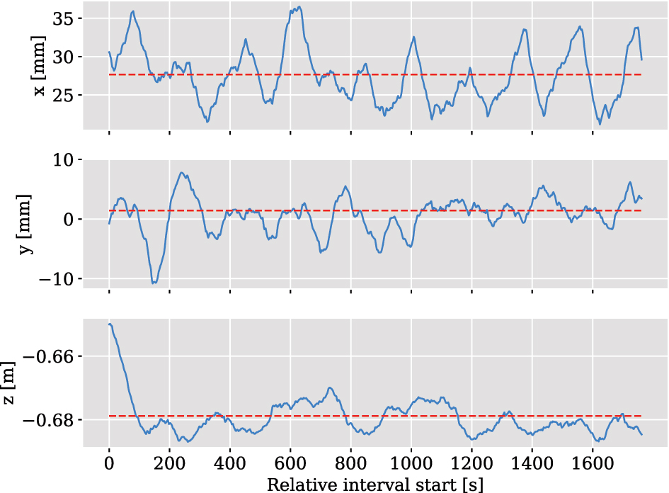
Stability of the estimated lever arm components derived using rolling one-minute intervals of observations. The overall estimation result is represented by the red line.
For example, deviations of the 360° prism depending on the angle of incidence of the total station signal could cause a deformation of its trajectory [20]. Another possibility are differences in the w-frames of both sensors, which were not taken into account during the alignment. Deviations in the measurement pillars used for the georeferencing of the total station could influence the lever arm in each lap similarly. The quality of the GNSS/IMU trajectory is mainly influenced by the GNSS quality, which is mostly systematic in nature and depends, among other factors, on the environment of the GNSS antenna.
Another peculiarity is the z-component of the lever arm. Compared to the entire measurement, the z-component is shorter at the beginning of the measurement. Starting with a deviation of about 3 cm, it steadily increases over a period of approximately 3 min. This could be related to the GNSS positioning, which can show systematic deviations especially in height.
4.4 Parameter correlation
The correlations of the estimated parameters, determined by using the a-posteriori variances, provide information about the extent to which individual parameters can be separated. In principle, the goal is to obtain a correlation of zero. The considerations from Section 2.3, which show that the properties of the trajectory play a decisive role, are of particular importance here.
Figure 7 shows the correlations for the spatio-temporal alignment of the hand-held measurement as a heatmap. Most noticeable are the high correlations between the lever arm and the translation of the similarity transformation. Especially the z-component is strongly correlated with 0.86. This is due to the fact that both parameters act in very similar directions. Only by tilting the s-frame relative to the w-frame, the influence of the z-component of the lever arm becomes different from the z-translation of the similarity transformation. Judging from the correlation, the tilting of the system during the measurement was not sufficient to allow a truly independent estimation of both parameters. For trajectories with little tilt variation, such as ground vehicles, it may be reasonable to estimate only one of the two parameters or, if possible, to measure the lever arm.
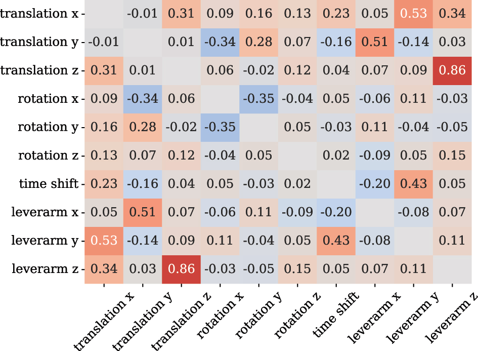
Resulting parameter correlations after spatio-temporal alignment of the hand-held trajectories.
The remaining values show that the correlations of the other parameters are significantly lower, but could not be completely eliminated. For example, the lever arm is correlated significantly with the translation of the similarity transformation and the time shift, indicating insufficient variation in the yaw angle. Even if completely uncorrelated parameters are rather hard to achieve with real data, the values obtained suggest that the measurement setup can be further optimized in future work.
For the spatio-temporal alignment of the manual rail-track measurement, the correlation between the time offset and the x-component of the lever arm is −0.65. This high correlation supports the hypothesis from Section 4.2 that the lack of varying vehicle orientations relative to the direction of travel complicates parameter separation. The correlations of the remaining parameters are approximately zero.
4.5 Trajectory evaluation
In this subsection, the determined alignment parameters are used to transform the GNSS/IMU trajectory to the total station ground truth trajectory. The transformed high-frequency GNSS/IMU trajectory is interpolated to the lower-frequency total station trajectory. By comparing both trajectories, the quality of the positions of the GNSS/IMU system can be examined. Since the total station provides only reference positions and no reference orientations, only the positioning of the GNSS/IMU system can be directly evaluated. However, because the orientations of the GNSS/IMU system were used in the alignment, their deviations are also indirectly included in the position deviations.
The upper part of Figure 8 shows the deviations between both trajectories of the hand-held measurement in histograms divided into along-, horizontal cross- and vertical cross-track directions. All three distributions scatter around zero, indicating successful alignment of the trajectories. This is because any systematic deviations in the positioning that can be described by Eq. (3) will be included in the estimated parameters. Conversely, this also means that constant deviations cannot be detected by comparison after alignment. If the GNSS/IMU system would always provide a globally shifted position, this offset would become part of the similarity transformation. Similarly, a constant deviation relative to the vehicle-fixed s-frame would be included in the lever arm. However, it should also be noted that changes in these systematic deviations can still be revealed. Furthermore, the estimated parameters of different measurement campaigns can be compared to assess the accuracy of the trajectory estimation.
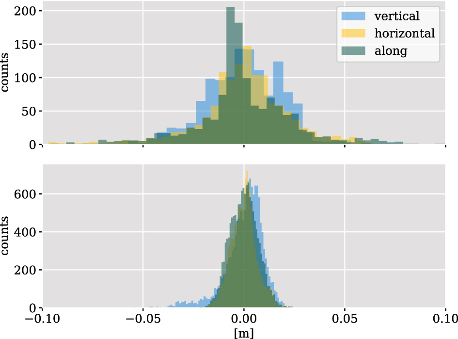
Deviations between the total station trajectory and the aligned GNSS/IMU trajectory for the hand-held measurement (top) and the rail-track measurement (bottom), divided into horizontal and vertical cross-track and along-track direction.
Examining the deviations, it is noticeable that the trajectory estimate scatters similarly in all three directions relative to the direction of travel. With a spread of approximately −5 to 5 cm, they exceed the manufacturer’s specifications of 2 cm in the horizontal position and 4 cm in height. This may be due to non-optimal RTK conditions, the rapid changes in orientation and direction or deviations in the spatio-temporal alignment.
The deviations of the rail measurement are shown in the lower part of Figure 8. Again, they are scattered around zero for the reasons discussed above. In contrast to the hand-held measurement, the deviations conform more closely to a normal distribution and fully meet the manufacturer’s specifications. In all three directions, the deviations range from about −2 cm to 2 cm. The qualitatively better results compared to the hand-held measurement could be a result of different GNSS conditions, the much more consistent shape of the rail-track, or a better alignment because of fewer parameters to estimate. There are isolated deviations in height of up to −4 cm, which is probably related to the irregularities of the height components already visible in Figure 6 at the beginning of the measurement.
5 Conclusion and outlook
In this paper, we presented a methodology for aligning two trajectories that can account for a similarity transformation, a lever arm transformation, and a time offset. The aligned trajectories can then be compared to each other to assess their quality. The proposed iterative least squares approach considers the stochastic properties of the observations and can be adapted to the individual requirements of an application by only estimating parameters that are actually unknown.
With the help of various experiments, the methodology was validated and experimentally evaluated. The measurements differed in shape, speed and the number of unknown alignment parameters. In each case, the trajectories were successfully aligned, as indicated by deviations around zero. It should be noted, however, that the approach presented here is based on actual measurements. This has the consequence that systematic deviations in the observations will affect the results of the alignment, which was particularly evident in the height component of the lever arm in the context of our studies. It is therefore advisable to repeat the alignment regularly at different times and under different conditions. This allows a system to be evaluated not only by comparing it with a reference but also by assessing the alignment parameters estimated in each case.
Furthermore, it became clear that the parameters could not always be fully separated from each other due to the nature of the recorded trajectories. High correlations occurred for parameters that similarly influence the alignment result. While this is not critical for stand-alone evaluation, it may be relevant if the actual values of the alignment parameters are of interest, e.g. in the context of a system calibration.
In future studies, an optimal trajectory shape or an alignment procedure could be determined that would provide the best possible parameter estimation. In addition, improving the stochastic model with respect to correlations would result in more realistic a-posteriori variances and better estimation results. Furthermore, the same spatio-temporal alignment could be used not only to compare but also to combine sensors. After alignment, a total station can be integrated into GNSS/IMU based trajectory estimation algorithms or even replace GNSS fully in certain situations.
Funding source: Deutsche Forschungsgemeinschaft
Award Identifier / Grant number: EXC 2070–390732324
-
Research ethics: Not applicable.
-
Informed consent: Not applicable.
-
Author contributions: Gereon Tombrink: Conceptualization, Methodology, Software, Validation, Investigation, Writing – Original Draft. Ansgar Dreier: Conceptualization, proof-reading. Lasse Klingbeil: Supervision, Conceptualization, proof-reading. Heiner Kuhlmann: Supervision, Conceptualization, Project administration. The authors have accepted responsibility for the entire content of this manuscript and approved its submission.
-
Use of Large Language Models, AI and Machine Learning Tools: None declared.
-
Conflict of interest: The authors state no conflict of interest.
-
Research funding: This work has been partially funded by the Deutsche Forschungsgemeinschaft (DFG, German Research Foundation) under Germany’s Excellence Strategy – EXC 2070–390732324.
-
Data availability: The raw data can be obtained on request from the corresponding author.
References
1. Geiger, A, Lenz, P, Urtasun, R. Are we ready for autonomous driving? The kitti vision benchmark suite. In: 2012 IEEE conference on computer vision and pattern recognition. IEEE; 2012:3354–61 pp.10.1109/CVPR.2012.6248074Suche in Google Scholar
2. Heinz, E, Eling, C, Klingbeil, L, Kuhlmann, H. On the applicability of a scan-based mobile mapping system for monitoring the planarity and subsidence of road surfaces – pilot study on the A44n motorway in Germany. J Appl Geodesy 2020;14:39–54. https://doi.org/10.1515/jag-2019-0016.Suche in Google Scholar
3. Olsen, MJ, Roe, GV, Glennie, C, Persi, F, Reedy, M, Hurwitz, D, et al.. Guidelines for the use of mobile LIDAR in transportation applications. Washington, DC, USA: TRB; 2013, TRB NCHRP Final Report 748.Suche in Google Scholar
4. Clausen, P, Gilliéron, P-Y, Perakis, H, Gikas, V, Spyropoulou, I. Positioning accuracy of vehicle trajectories for road applications. Bordeaux: ITS World Congress 2015; 2015.Suche in Google Scholar
5. Cramer, M, Stallmann, D, Haala, N. Direct georeferencing using gps/inertial exterior orientations for photogrammetric applications. Int Arch Photogramm Remote Sens 2000;33:198–205.Suche in Google Scholar
6. Quan, Y, Lau, L. Development of a trajectory constrained rotating arm rig for testing GNSS kinematic positioning. Measurement 2019;140:479–85. https://doi.org/10.1016/j.measurement.2019.04.013.Suche in Google Scholar
7. Tombrink, G, Dreier, A, Klingbeil, L, Kuhlmann, H. Trajectory evaluation using repeated rail-bound measurements. J Appl Geodesy 2023;17:205–16. https://doi.org/10.1515/jag-2022-0027.Suche in Google Scholar
8. Zhang, Z, Scaramuzza, D. A tutorial on quantitative trajectory evaluation for visual(-inertial) odometry. In: 2018 IEEE/RSJ international conference on intelligent robots and systems (IROS); 2018:7244–51 pp.10.1109/IROS.2018.8593941Suche in Google Scholar
9. Horn, BK. Closed-form solution of absolute orientation using unit quaternions. Josa A 1987;4:629–42. https://doi.org/10.1364/josaa.4.000629.Suche in Google Scholar
10. Umeyama, S. Least-squares estimation of transformation parameters between two point patterns. IEEE Trans Pattern Anal Mach Intell 1991;13:376–80. https://doi.org/10.1109/34.88573.Suche in Google Scholar
11. Cramer, M. Direct geocoding: is aerial triangulation obsolete; fritsch/spiller (eds.), photographic week 1999. Heidelberg, Germany: Wichmann Verlag; 1999:59–70 pp.Suche in Google Scholar
12. Gao, Y, Meng, X, Hancock, CM, Stephenson, S, Zhang, Q. Uwb/gnss-based cooperative positioning method for v2x applications. In: Proceedings of the 27th international technical meeting of the satellite division of the institute of navigation (ION GNSS+ 2014); 2014:3212–21 pp.Suche in Google Scholar
13. Geiger, A, Lenz, P, Stiller, C, Urtasun, R. Vision meets robotics: the kitti dataset. Int J Robot Res 2013;32:1231–7. https://doi.org/10.1177/0278364913491297.Suche in Google Scholar
14. Gikas, V, Perakis, H. Rigorous performance evaluation of smartphone gnss/imu sensors for its applications. Sensors 2016;16:1240. https://doi.org/10.3390/s16081240.Suche in Google Scholar PubMed PubMed Central
15. Vogel, S, Hake, F. Development of gps time-based reference trajectories for quality assessment of multi-sensor systems. J Appl Geodesy 2024;18:597–612. https://doi.org/10.1515/jag-2023-0084.Suche in Google Scholar
16. Koch, K-R. Parameter estimation in linear models. Berlin, Heidelberg: Springer; 1999:149–269 pp.10.1007/978-3-662-03976-2_4Suche in Google Scholar
17. Niemeier, W. Ausgleichungsrechnung: statistische Auswertemethoden. Berlin: Walter De Gruyter; 2008.10.1515/9783110206784Suche in Google Scholar
18. Teunissen, PJG. Adjustment theory: An introduction. Delft: TU Delft OPEN Publishing; 2024.10.59490/tb.95Suche in Google Scholar
19. Thalmann, T, Neuner, H. Temporal calibration and synchronization of robotic total stations for kinematic multi-sensor-systems. J Appl Geodesy 2021;15:13–30. https://doi.org/10.1515/jag-2019-0070.Suche in Google Scholar
20. Lackner, S, Lienhart, W. Impact of prism type and prism orientation on the accuracy of automated total station measurements. In: Proc. 3rd joint international symposium on deformation monitoring. Vienna; 2016.Suche in Google Scholar
© 2024 the author(s), published by De Gruyter, Berlin/Boston
This work is licensed under the Creative Commons Attribution 4.0 International License.
Artikel in diesem Heft
- Frontmatter
- Original Research Articles
- Locally robust Msplit estimation
- Extending geodetic networks for geo-monitoring by supervised point cloud matching
- Evaluation and homogenization of a marine gravity database from shipborne and satellite altimetry-derived gravity data over the coastal region of Nigeria
- Modelling geoid height errors for local areas based on data of global models
- Unmanned aerial vehicle-based aerial survey of mines in Shanxi Province based on image data
- Ionospheric TEC and its irregularities over Egypt: a comprehensive study of spatial and temporal variations using GOCE satellite data
- Monitoring of volcanic precursors using satellite data: the case of Taftan volcano in Iran
- Modeling of temperature deformations on the Dnister HPP dam (Ukraine)
- Impact of temporal resolution in global ionospheric models on satellite positioning during low and high solar activity years of solar cycle 24
- Comparative performance of PPP software packages in atmospheric delay estimation using GNSS data
- Assessment and fitting of high/ultra resolution global geopotential models using GNSS/levelling over Egypt
- An efficient ‘P1’ algorithm for dual mixed-integer least-squares problems with scalar real-valued parameters
- Spatio-temporal trajectory alignment for trajectory evaluation
- Monitoring of networked RTK reference stations for coordinate reference system realization and maintenance – case study of the Czech Republic
- Crustal deformation in East of Cairo, Egypt, induced by rapid urbanization, as seen from remote sensing and GNSS data