An efficient ‘P1’ algorithm for dual mixed-integer least-squares problems with scalar real-valued parameters

Lotfi Massarweh; Peter J. G. Teunissen

doi:10.1515/jag-2024-0076

Article Open Access

An efficient ‘P1’ algorithm for dual mixed-integer least-squares problems with scalar real-valued parameters

Lotfi Massarweh and Peter J. G. Teunissen

Published/Copyright: December 4, 2024

Published by

Become an author with De Gruyter Brill

Submit Manuscript Author Information

From the journal Journal of Applied Geodesy Volume 19 Issue 2

Abstract

In this contribution we consider mixed-integer least-squares problems, where the integer ambiguities a ∈ Z n and real-valued parameters b ∈ R p are estimated. Both a primal and a dual formulation can be considered, with the latter concerning the ambiguity resolution process taking place into the parameters’ domain. We study the p = 1 case, where an ad hoc ‘P1’ algorithm is introduced, and some geometrical insights are provided. It is demonstrated how the algorithm’s complexity (i.e. number of candidate integer solutions to be evaluated) grows linearly with the ambiguity dimensionality n, differently from the primal formulation where an exponential growth is observed. By means of numerical simulations, here based on Global Navigation Satellite System (GNSS) models, we show the efficiency of this proposed ‘P1’ algorithm, meanwhile also demonstrating its quasi-optimal statistical performance.

Keywords: GNSS; ambiguity resolution; integer least-squares (ILS); dual mixed ILS; deterministic global optimization; P1 algorithm

1 Introduction

The Integer Ambiguity Resolution (IAR) process concerns the successful resolution of the unknown integer ambiguities present in mixed-integer models. For instance, in the context of Global Navigation Satellite Systems (GNSS), carrier-phase IAR is the key to fast and high-precision baseline estimation [1]. Once these ambiguities have been correctly resolved, the carrier-phase data starts acting as very precise pseudo-range data, so enabling users’ precise positioning and navigation, see [2], 3].

When considering mixed-integer least-squares problems, two equivalent formulations are possible, denoted as primal and dual, respectively introduced by Teunissen [4] and by Teunissen and Massarweh [5]. In the primal formulation, integer ambiguities are firstly resolved followed by a conditional least-squares baseline estimator, so computing ambiguity-fixed baseline solutions. Efficient algorithms exist for tackling such IAR problems within the ambiguity domain, for instance with the Least-Squares AMBiguity Decorrelation Adjustment (LAMBDA) method, see [6]. On the other hand, in the dual formulation, the IAR process takes place directly in the parameters’ domain and globally convergent solutions could be defined, as presented by Teunissen and Massarweh [5].

In this contribution we further study dual mixed-ILS problems, focusing on the case p = 1, i.e. scalar real-valued parameter b ∈ R , meanwhile assuming an arbitrary number of integer ambiguity components in a ∈ Z n , n ≥ 1. A deterministic P1 algorithm is introduced here as an efficient implementation for the ambiguity search process, now taking place in the parameters’ domain [7]. By defining the algorithm complexity as ‘number of candidate solutions evaluated’, it is demonstrated that, in the dual formulation (for p = 1), the complexity grows linearly with the dimensionality n. Besides the numerical performance, compared here against LAMBDA method, we also investigate statistical performances, thus showing that quasi-optimal solutions can be obtained by the P1 algorithm.

In Section 2, a brief review of dual mixed-integer least-squares models is given, then focusing on the case n ≥ p = 1. In Section 3, the P1 algorithm is presented, along with some geometrical insights, and the linear growth of complexity with respect to the dimensionality n is demonstrated. The performance is numerically investigated in Section 4, i.e. considering GNSS models, while the main conclusions are summarized in Section 5.

2 Review of dual mixed ILS models

The dual formulation for mixed-integer least-squares models was introduced by Teunissen and Massarweh [5]. We start here with the observables’ vector y ∈ R m , so

(1) y ∼ N m A a + B b , Q y y , a ∈ Z n , b ∈ R p

where ∼ refers to distributed as, given an m-dimensional normal distribution with expectation E y = A a + B b and dispersion D y = Q y y for Q y y ∈ R m × m being the variance-covariance of y. The full-rank design matrix is given by A , B ∈ R m × n + p , while integer ambiguities and real-valued parameters are respectively denoted as a and b.

The dual formulation considers a dual objective function D : R p → R given by

(2) D b = b − b ̂ Q b ̂ b ̂ 2 + a ̂ b − a ̆ b Q a ̂ b 2

where the (dual) mixed ILS solution for the real-valued parameters follows as

(3) b ̆ = arg min b ∈ R p D b

given the (conditioned) ambiguity vectors

(4) a ̂ b = a ̂ − Q a ̂ b ̂ Q b ̂ b ̂ b ̂ − b , a ̆ b = arg min a ∈ Z n | | a ̂ b − a | | Q a ̂ b 2

with Q a ̂ b ∈ R n × n as conditional variance-covariance matrix of ambiguities. The latter ones are conditioned onto the current b-value that could freely be defined in R p .

Two approximations of Eq. (2) are discussed in (ibid), such as

Approximate weighting, where we replace the conditional variance matrix Q a ̂ b by an approximation Q a ̂ b ◦ , e.g. diagonal matrix, such that
(5) D ◦ b = b − b ̂ Q b ̂ b ̂ 2 + a ̂ b − a ̆ ◦ b Q a ̂ b ◦ 2
for a ̆ ◦ b = arg min a ∈ Z n | | a ̂ ( b ) − a | | Q a ̂ b ◦ 2 .
Approximate mapping, where we replace the integer minimizer of Eq. (4) by an arbitrary admissible estimator I • : R n → Z n , e.g. integer rounding, such that
(6) D • b = b − b ̂ Q b ̂ b ̂ 2 + a ̂ b − I • a ̂ b Q a ̂ b 2
and the two approximations differ since in the ‘approximate weighting’ case we neglect off-diagonal terms in Q a ̂ b , whereas in the ‘approximate mapping’ case we might adopt simpler rounding estimators for the many-to-one mapping function I • .

2.1 Particular case for n ≥ p = 1

We focus on the case p = 1, thus defining β ∈ R and D : R → R , where

(7) D β = D 1 β + D 2 β = β − b ̂ 2 σ b ̂ 2 + a ̂ β − a ̆ β Q a ̂ b 2

for a ̂ β = a ̂ − q a ̂ b ̂ σ b ̂ − 2 b ̂ − β given q a ̂ b ̂ ∈ R n , while a ̆ β follows Eq. (4). Note that in the parameter domain the dual objective function is composed by a parabolic term D 1 β and a periodic-like term D 2 β , as shown in Figure 5 by Teunissen and Massarweh [5]. At the same time, in the ambiguity domain we are able to define ‘pull-in regions’, i.e. subsets of R n where float vectors are mapped to the corresponding integer.

For integer estimators, the pull-in regions are translational invariant over the integers and cover the entire space R n without gaps and overlaps [8], 9]. Moreover, from Eq. (7), we observe that potential integer candidates are the ones belonging to pull-in regions crossed by the conditioned line a ̂ β for β ∈ R . In Figure 1, we provide an illustrative example for p=1, n=2 given β ∈ β MIN = b ̂ − 1.7 , β MAX = b ̂ + 1.7 , with these bounds for β further specified later, where

(8) a ̂ 1 a ̂ 2 b ̂ = + 0.4 − 0.6 + 0.2 , σ a ̂ 1 2 σ a ̂ 1 a ̂ 2 σ a ̂ 1 b ̂ σ a ̂ 2 a ̂ 1 σ a ̂ 2 2 σ a ̂ 2 b ̂ σ b ̂ a ̂ 1 σ b ̂ a ̂ 2 σ b ̂ 2 ≅ + 0.733 − 0.666 + 0.294 − 0.666 + 1.031 − 0.637 + 0.294 − 0.637 + 0.490 ,

such that q a ̂ b ̂ = σ b ̂ a ̂ 1 , σ b ̂ a ̂ 2 T , and therefore

(9) Q a ̂ b = Q a ̂ a ̂ − q a ̂ b ̂ q a ̂ b ̂ T σ b ̂ − 2 ≅ + 0.557 − 0.284 − 0.284 + 0.203 , Q a ̂ b ◦ ≅ 0.557 0 0 0.203

with two pull-in regions represented in red and blue respectively when using Q a ̂ b and its diagonal approximation Q a ̂ b ◦ as inverse-weighting matrix. In the first case (in red), we are looking at Integer Least-Squares pull-in regions (i.e. hexagons), while in the second case (in blue) we have more simple Integer Rounding pull-in regions (i.e. unit squares).

$Figure 1: The conditioned line a ̂ β $\hat{a}\left(\beta \right)$ is shown in magenta given β ∈ β MIN , β MAX $\beta \in \left[{\beta }_{\text{MIN}},{\beta }_{\text{MAX}}\right]$ , i.e. defined between the extreme points a ̂ β MIN $\hat{a}\left({\beta }_{\text{MIN}}\right)$ and a ̂ β MAX $\hat{a}\left({\beta }_{\text{MAX}}\right)$ . The magenta circle refers to a ̂ b $\hat{a}\left(b\right)$ for the true b ∈ R $b\in \mathbb{R}$ , while the asterisk refers to a ̂ ( b ̂ ) ≡ a ̂ $\hat{a}\left(\hat{b}\right)\equiv \hat{a}$ , i.e. the float ambiguity solution. Moreover, two pull-in regions are defined as hexagons (in red) or unit squares (in blue) when making use of Q a ̂ b ${Q}_{\hat{a}\left(b\right)}$ or Q a ̂ b ◦ ${Q}_{\hat{a}\left(b\right)}^{{\circ}}$ as inverse-weighting matrix, respectively.$

Figure 1:

The conditioned line a ̂ β is shown in magenta given β ∈ β MIN , β MAX , i.e. defined between the extreme points a ̂ β MIN and a ̂ β MAX . The magenta circle refers to a ̂ b for the true b ∈ R , while the asterisk refers to a ̂ ( b ̂ ) ≡ a ̂ , i.e. the float ambiguity solution. Moreover, two pull-in regions are defined as hexagons (in red) or unit squares (in blue) when making use of Q a ̂ b or Q a ̂ b ◦ as inverse-weighting matrix, respectively.

The weighting approximation leads to an approximate dual objective function

(10) D ◦ β = D 1 β + D 2 ◦ β = β − b ̂ 2 σ b ̂ 2 + a ̂ β − a ̆ ◦ β Q a ̂ b ◦ 2

so using D ◦ β instead of D β , both illustrated in Figure 2, with a common parabolic term D 1 highlighted in green color. The periodic-like terms D 2 and D 2 ◦ are depicted in red and blue colors, as for their pull-in regions, respectively on the left and right side. Note that when Q a ̂ b is diagonal, no approximation takes place at all, and the original dual problem is being considered. Even if Q a ̂ b is diagonal, it does not imply that also Q a ̂ a ̂ is diagonal, and in the primal formulation we might deal with highly correlated (unconditioned) ambiguities.

$Figure 2: The dual objective function D β $\mathcal{D}\left(\beta \right)$ and its approximation D ◦ β ${\mathcal{D}}^{{\circ}}\left(\beta \right)$ are shown in the left and right plots, respectively, with the parabolic term D 1 β ${\mathcal{D}}_{1}\left(\beta \right)$ shown as green dashed line. The periodic-like contributions D 2 β ${\mathcal{D}}_{2}\left(\beta \right)$ and D 2 ◦ β ${\mathcal{D}}_{2}^{{\circ}}\left(\beta \right)$ are respectively given in red and blue, as well as their pull-in regions, while the conditioning line a ̂ β $\hat{a}\left(\beta \right)$ is depicted in magenta, centered in a ̂ b ̂ ≡ a ̂ $\hat{a}\left(\hat{b}\right)\equiv \hat{a}$ (magenta asterisk), where we have D 1 b ̂ = 0 ${\mathcal{D}}_{1}\left(\hat{b}\right)=0$ .$

Figure 2:

The dual objective function D β and its approximation D ◦ β are shown in the left and right plots, respectively, with the parabolic term D 1 β shown as green dashed line. The periodic-like contributions D 2 β and D 2 ◦ β are respectively given in red and blue, as well as their pull-in regions, while the conditioning line a ̂ β is depicted in magenta, centered in a ̂ b ̂ ≡ a ̂ (magenta asterisk), where we have D 1 b ̂ = 0 .

The required interval β MIN , β MAX can be found starting with an initial guess β 0 = def b ̂ , so leading to a ̂ β 0 = a ̂ , and then seeking new solutions β_j for j > 0, such that

(11) D β j ≤ D β 0 = a ̂ − a ̆ β 0 Q a ̂ b 2

and therefore

(12) b ̂ − β j 2 σ b ̂ 2 ≡ D 1 β j ≤ D β j → Eq. 11 b ̂ − β j 2 σ b ̂ 2 ≤ D β 0

where the first inequality follows from the definition of D β , see Eq. (7). Hence, we are able to define an initial search radius R 0 = σ b ̂ D β 0 such that − R 0 ≤ β j − b ̂ ≤ R 0 for any j-th candidate solution, i.e. interval b ̂ − R 0 , b ̂ + R 0 is found. A grid search could be performed over this interval, but in this work we will consider an alternative efficient approach for the enumeration of all potential solutions, as discussed next.

3 The P1 algorithm

In the earlier Figure 1 we notice how several β values might belong to the same pull-in regions, implying that a grid search might be inefficient. At the same time, pull-in regions are convex regions for any n > 0, and the conditioning line a ̂ β will at most intersect them twice. By identifying any β value associated with each different integer vector a ̆ β , we could obtain a finite set of integer candidates where we expect to find a global minimizer. This is the main idea behind the ‘P1’ algorithm described in this section.

The intersection between a ̂ β and ILS pull-in regions is not trivial, therefore we will restrict our discussion to the approximated dual objective function D ◦ β . Hence, we make use of Q a ̂ b ◦ after neglecting the off-diagonal terms of Q a ̂ b , but notice that in some mixed-integer models the latter one might already be a diagonal matrix, as discussed later. Based on the example of Figure 1, we can consider again an illustration of the conditioning line a ̂ β for β ∈ β MIN , β MAX given in magenta color in the Figure 3 (note a rotated plot). The intersections with each interface (of unit-square regions) are shown by magenta squares, while the middle points β j MP are computed between two consecutive intersections, here shown as (filled) blue hexagrams. Each candidate β j MP will belong to an individual rounding pull-in region.

$Figure 3: Illustration of the example p = 1, n = 2, from Figure 1, with the conditioning line a ̂ β $\hat{a}\left(\beta \right)$ in magenta color given β ∈ β MIN , β MAX $\beta \in \left[{\beta }_{\text{MIN}},{\beta }_{\text{MAX}}\right]$ . The intersections with all interfaces are shown as magenta squares, while the middle points β j MP ${\beta }_{j}^{\text{MP}}$ are given as (filled) blue hexagrams.$

Figure 3:

Illustration of the example p = 1, n = 2, from Figure 1, with the conditioning line a ̂ β in magenta color given β ∈ β MIN , β MAX . The intersections with all interfaces are shown as magenta squares, while the middle points β j MP are given as (filled) blue hexagrams.

3.1 Algorithm description

The P1 algorithm starts with an initial search radius R₀ and we consider individually each i-th component of the conditioned ambiguity vector. By making use of the expression of the conditioned line a ̂ β projected along each component, i.e. a ̂ i β = a ̂ i + q a ̂ i b ̂ σ b ̂ − 2 β − b ̂ , it is then possible to bound each i-th term since β − b ̂ ∈ − R 0 , + R 0 , so having

(13) a ̂ i β ∈ a ̂ i − Δ i , a ̂ i + Δ i , Δ i = def q a ̂ i b ̂ σ b ̂ 2 R 0

where q a ̂ i b ̂ refers to the i-th component of the vector q a ̂ b ̂ ∈ R n . In this way, we can compute all the integer components ν i ∈ Z between a ̂ i − Δ i and a ̂ i + Δ i , and define values β ν i that are related to the interfaces with rounding pull-in regions. These values are then collected from all i-th ambiguity components in one sorted list, i.e. β MIN , … , β j − 1 , β j , β j + 1 , … , β MAX , while also including both two extrema β MIN = b ̂ − R 0 and β MAX = b ̂ + R 0 .

The middle point can be found by β j MP = b j + b j + 1 / 2 , and will belong to a single integer pull-in region, hence refers to an individual integer candidate u j = def a ̆ ◦ β j MP ∈ Z n . In the solutions’ evaluation process, we can start with values β j MP that are closer to b ̂ , since they will be associated with a smaller parabolic term D 1 β j MP . Moreover, during the evaluations, we can make use of results from Eq. (12) in order to reduce the search radius R₀ after each evaluation. This leads to discarding several outer values of β that could not further minimize the dual objective function.

This search-and-shrink strategy is similar to the primal counterpart already adopted in LAMBDA, but now we ‘shrink’ the real-valued parameters’ domain (i.e. on the conditioning line) where the enumeration process takes place. Once all potential candidates in the current interval are evaluated, the process stops and the global minimum β* is obtained. A summary of ‘P1’ algorithm is given in Algorithm 1, which consists of three parts: INITIALIZATION where an initial guess allows computing the initial search radius R₀, ENUMERATION of the integer candidates that are found inside the initial interval, and MAIN SEARCH, where such potential solutions are evaluated, including the aforementioned ‘shrinking’ strategy.

Algorithm 1:

Summary of the ‘P1’ algorithm described in Section 3.1

INPUTS:

a ̂ ∈ R n , b ̂ ∈ R , Q a ̂ a ̂ ∈ R n × n , q a ̂ b ̂ ∈ R n , σ b ̂ ∈ R

INITIALIZATION:

Given β 0 = b ̂ (initial guess), compute a ̂ β 0 = a ̂ based on Eq. (4), which is used to find a ̆ 0 ◦ = a ̂ ∈ Z n , along with an initial search radius R 0 = σ b ̂ D ◦ b ̂ a ̆ 0 ◦ .

ENUMERATION: % Find all potential integer candidates

For each i-th ambiguity component a ̂ i , with i = 1, …, n, find the intersections with rounding pull-in regions given ν i ∈ Z ∩ a ̂ i − Δ i , a ̂ i + Δ i , see Eq. (13)

Collect all β-values in one sorted list: β MIN , … , β j , … , β MAX , so including the extrema β MIN = b ̂ − R 0 and β MAX = b ̂ + R 0 .

Compute the middle points β j MP = b j + b j + 1 / 2 , each associated to a single integer candidate, and sorted now starting from smaller values of β j MP − b ̂ .

MAIN SEARCH: % Evaluate each potential integer candidate

Set D * as the current best function value from the step INITIALIZATION, with the current best solution defined by β * = b ̂ a ̆ 0 ◦ .

% Iterate over each j-th potential solution, sorted by β j MP − b ̂ .

for j = 1, …, N

% Outside the interval, search is over.

if β j MP − b ̂ > R 0

Break loop;

end

% Evaluation of the current integer candidate.

Compute the integer vector u j = def a ̆ ◦ β j MP = a ̂ β j MP , which it is used to evaluate a new objective function D j NEW = D ◦ b ̂ u j , see Eq. (15).

% Update the current best solution

if D j NEW < D *

Save D * = D j NEW and β * = β j NEW = b ̂ u j ;

% Shrinking step, see Eq. (12)

Update current R₀ (search radius);

end

OUTPUTS:

β * ∈ R , a ̆ ◦ β * ∈ Z n , D * ∈ R

NOTE: the symbol ⌈·⌋ defines the integer rounding operator.

In Algorithm 1, the main search takes place starting with smaller values β j MP − b ̂ , then considering that β j MP − b ̂ ≤ β j + 1 MP − b ̂ for any j > 0. Therefore, once the j-th solution is found outside the interval b ̂ − R 0 , b ̂ + R 0 , given the current radius R₀ (updated after each evaluation), we can stop the for-loop iterations. For the evaluation of each integer candidate u j = def a ̆ ◦ β j MP , we might directly exploit a primal formulation, thus evaluating

(14) P ◦ u j = | | a ̂ − u j | | Q a ̂ a ̂ ◦ 2 , b ̆ = def b ̂ u j = b ̂ − q a ̂ b ̂ T Q a ̂ a ̂ ◦ − 1 a ̂ − u j

given the approximate primal objective function P ◦ : Z n → R for Q a ̂ a ̂ ◦ = Q a ̂ b ◦ + q a ̂ b ̂ q a ̂ b ̂ T / σ b ̂ 2 , so following Lemma 4 by Teunissen and Massarweh [5].

On the other hand, the candidates’ evaluation could also be performed directly in the dual formulation, starting from a selected integer value u ∈ Z n . Using Lemma 7 from (ibid), we know that the local minimizer for a ̂ β ∈ S u , i.e. pull-in region of u such that a ̆ ◦ β = u , can be computed based on a primal conditioning b ̂ u = b ̂ − q a ̂ b ̂ T Q a ̂ a ̂ ◦ − 1 a ̂ − u , where

(15) P ◦ u = D ◦ b ̂ u , ∀ u ∈ Z n

so now evaluating D ◦ and no other minima exist given a ̂ β ∈ S u , see (ibid). In this way it is possible to initialize using Q a ̂ a ̂ ◦ rather than Q a ̂ b ◦ , so leading to fewer integer candidates.

3.2 Algorithm complexity

Before presenting a numerical analysis of the performance, we can briefly discuss the linear growth of complexity, here defined by the number of potential candidates that are evaluated during the enumeration process. In fact, in the dual formulation with D ◦ β , the algorithm’s complexity can be shown to be linearly increasing with the dimensionality n > 0.

Starting with Eq. (13), we can approximate a maximum number of candidates of each i-th component directly using N i MAX ≅ 2 Δ i , such that the total number of candidates (i.e. the middle points computed between successive intersections) follows as

(16) N MAX = ∑ i = 1 i = n N i MAX ≅ ∑ i = 1 i = n 2 R 0 q a ̂ i b ̂ σ b ̂ 2 = 2 R 0 σ b ̂ 2 ∑ i = 1 i = n q a ̂ i b ̂

where the approximation ≅ gets more accurate for larger values of N i MAX , i = 1 , … , n .

Given that q a ̂ i b ̂ = ρ a ̂ i b ̂ σ a ̂ i σ b ̂ for the correlation term ρ a ̂ i b ̂ ∈ − 1 , + 1 , we notice that each N i MAX grows with the (unconditioned) standard deviation σ a ̂ i of the i-th ambiguity component a ̂ i , which is dependent on the underlying model strength. Note that the search of a global minimum will take around N^MAX evaluations of all the middle points β j MP currently in the list, meanwhile we continue here by defining

(17) q a ̂ i b ̂ ̄ = 1 n ∑ i = 1 i = n q a ̂ i b ̂

and we further reformulate the approximation in Eq. (16) as

(18) N MAX ≅ 2 R 0 σ b ̂ 2 n q a ̂ i b ̂ ̄

where q a ̂ i b ̂ ̄ is smaller than the largest entry (in absolute value) of q a ̂ b ̂ ∈ R n . This shows how N^MAX grows linearly with the dimensionality n given an initial search radius R₀, which can be computed based on Eq. (11), e.g. using R 0 = σ b ̂ D β 0 , therefore we obtain

(19) N MAX ≅ 2 n ⋅ D β 0 ⋅ q a ̂ i b ̂ ̄ σ b ̂

and the complexity is indeed dependent upon three elements: the problem dimensionality, the initial guess β₀ and the variance/covariance terms. Note that given q a ̂ i b ̂ ̄ = 0 , no correlation exists at all between the float ambiguities a ̂ i and the parameter b ̂ , so the latter is actually the global minimizer for our dual problem.

4 Numerical assessments

We start by a simple numerical example for a multi-frequency geometry-free model, where the conditional variance matrix Q a ̂ b is diagonal, whereas the unconditional matrix Q a ̂ a ̂ is not. Given a single-epoch single-baseline ionosphere-fixed scenario, two receivers track two Galileo satellites based on a standard deviation of σ_p = 30 cm and σ_ϕ = 3 mm respectively for the undifferenced code and phase observations.

The mixed-integer model of Eq. (1), given J frequencies, is based on

(20) A = 0 Λ J , B = e J e J , Q y y = 4 σ p 2 I J σ ϕ 2 I J

where I J ∈ Z J × J refers to the identity matrix, e J ∈ Z J is a vector of 1s, while Λ J ∈ R J × J is a diagonal matrix with its entries as the signal wavelengths, where n = J. The factor ‘4’ arises from the covariance propagation law following the double-differencing operator for code and phase observables.

We consider four scenarios based on Galileo signal, i.e. E1 + E6 (n = 2), E1 + E6 + E5a (n = 3) E1 + E6 + E5a + E5b (n = 4) and E1 + E6 + E5a + E5b + E5 (n = 5), where computational time over 2,000 different samples has been presented in Figure 4. In all these simulations, the results for p = 1 using the P1 algorithm perfectly match with the ILS solutions computed by LAMBDA 4.0 toolbox [10], since Q a ̂ b is a diagonal matrix, where

(21) Q a ̂ b − 1 = A T Q y y − 1 A = Λ J T Λ J 4 σ ϕ 2 = 1 4 σ ϕ 2 diag λ 1 2 , … , λ J 2

therefore no approximation takes place in our dual formulation, and

(22) D β ≡ D ◦ β = n β − b ̂ 2 4 σ p 2 + 1 4 σ ϕ 2 ∑ i = 1 i = n λ i 2 ε ̆ i 2 β , ∀ β ∈ R

for the ambiguity residuals’ defined by ε ̆ i β = a ̂ i β − a ̂ i β for i = 1, …, n and ⌈·⌋ being the integer rounding operation. Notice how the parabolic term D 1 and periodic-like term D 2 are mainly driven by the precision of code and phase measurements, respectively. Moreover, in this illustrative example, we observe a smaller computational time for the P1 algorithm with respect to LAMBDA method, and its efficiency becomes more visible when increasing the ambiguity problem dimensionality.

Figure 4:

The computational times for primal (ILS) and dual (P1) solutions are shown given four different Galileo scenarios, i.e. E1 + E6 (n = 2, top left), E1 + E6 + E5a (n = 3, top right) E1 + E6 + E5a + E5b (n = 4, bottom left) and E1 + E6 + E5a + E5b + E5 (n = 5, bottom right). For each scenario, we use 2,000 different float samples, see text for more information.

Based on 2,000 samples (n = 3), we show in Figure 5 the maximum number of integer candidates (in blue) as defined by Eq. (16), which seems to well approximate the potential number of candidates (in orange) iterated in the MAIN SEARCH step (see Algorithm 1), i.e. number of middle points previously found in ENUMERATION. However, by means of the search-and-shrink approach, we note that the actual number of integer candidates evaluated (in yellow) is substantially reduced. This demonstrates substantial improvements in terms of efficiency once accounting for a search-and-shrink strategy in the ‘P1’ algorithm, as adopted in the numerical results of Figure 4.

Figure 5:

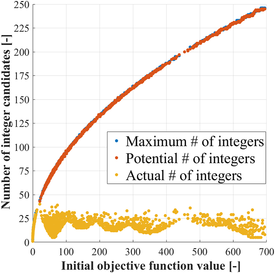
The maximum number of expected integer candidates is shown (in blue) based on the Eq. (16), while the potential number of integers refers to middle points (in orange) actually computed in this analysis over 2,000 different samples for n = 3. Lastly, we also provide the actual total number of integers being evaluated (in yellow), largely reduced thanks to the search-and-shrink strategy adopted by the ‘P1’ algorithm.

At this point, we continue with a different numerical example, where the matrix Q a ̂ b is not diagonal and suboptimal performance (with respect to a primal ILS estimator) might be expected, so we focus on statistical performances rather than computational ones.

4.1 Statistical performance for Q a ̂ b not diagonal

We consider a single-epoch single-baseline geometry-based ionosphere-fixed model, with m satellites tracked on GPS L1 frequency. We assume the horizontal position known, leading to p = 1 estimation of the vertical (UP) coordinate b UP ∈ R , where

(23) A = 0 λ 1 I m − 1 , B = D m T G D m T G , Q y y = 2 D m T Q p p D m D m T Q ϕ ϕ D m

with I n ∈ Z n × n refers to the identity matrix for n = m − 1, while D m T = − e m − 1 , I m − 1 is the between-satellite single differencing with respect to the first (pivot) satellite, and the vector G ∈ R m consists of sin el ° terms for each GPS satellite, see [11].

The stochastic model follows by a covariance propagation law for the undifferenced code and phase standard deviation (at zenith), respectively given as 30 cm and 3 mm, while an elevation weighting ∝ 1 / sin el ° is adopted. Therefore, both matrices Q_ϕϕ and Q_pp are diagonal with entries being the elevation-dependent standard deviations. Note that a term ‘2’ in the expression for Q_yy arises from the between-receiver differencing.

At this point, given Q a ̂ a ̂ ◦ , we aim to analyze such dual approximation of the variance-covariance matrix Q a ̂ a ̂ for the estimated (unconditioned) float ambiguities. The objective is to assess how accurate the dual approximation is, where as a matter of comparison we will consider also a primal approximation given Q a ̂ a ̂ ⊙ . Three different scenarios are compared:

Case #1: We use Q a ̂ a ̂ = Q a ̂ b + Q a ̂ b ̂ Q b ̂ b ̂ − 1 Q b ̂ a ̂ ;
Case #2: We use Q a ̂ a ̂ ◦ = Q a ̂ b ◦ + Q a ̂ b ̂ Q b ̂ b ̂ − 1 Q b ̂ a ̂ , with Q a ̂ b ◦ diagonal;
Case #3: We use Q a ̂ a ̂ ⊙ = Q a ̂ b + Q a ̂ b ̂ Q b ̂ b ̂ − 1 Q b ̂ a ̂ ⊙ , with Q a ̂ a ̂ ⊙ diagonal;

where in the Case #1, we consider a (primal) Integer Least-Squares solution based on the full variance-covariance matrix Q a ̂ a ̂ , in the Case #2 we adopt a dual approximation based on Q a ̂ a ̂ ◦ where Q a ̂ b ◦ accounts only for the diagonal entries of Q a ̂ b (that is not diagonal), while in the Case #3 we consider a (primal) Integer Rounding solution based on Q a ̂ a ̂ ⊙ , being the diagonal matrix extracted from Q a ̂ a ̂ . In LAMBDA, a decorrelation process [6] is used to reduce the correlation between (unconditioned) float ambiguities, based on an admissible transformation matrix Z ∈ Z n × n (unimodular), so z ̂ = Z T a ̂ . Still, in order to directly compare statistical performances of these three cases, no ambiguity decorrelation has been used here, while in Case #1 such a re-parametrization would only affect the computational time.

In Figure 6, the errors for the ‘UP’ component are shown using 6,000 samples, where a total of 8 satellites has been tracked, i.e. n = 7. In grey color, the float solution is illustrated, having a standard deviation σ b ̂ ≅ 1.612 [m], while the fixed results are presented in green and red color referring to correctly fixed and incorrectly fixed ambiguities, respectively. The success rate (SR) is computed for the three scenarios, with SR ≅ 97.9 %, ≅97.0 %, ≅6.3 % for each case. The poor success rate of the primal rounding is visible in the large UP errors, with a root mean squares (RMS) value of around 1.6 [m] in contrast to the 1.6 [cm] found for the fixed solutions when ambiguities are correctly resolved, i.e. a = 0 (in green).

Figure 6:

The ‘UP’ error component [m] is shown for different samples generated based on a single-epoch single-baseline geometry-based ionosphere-fixed model for L1 signal tracked by 8 GPS satellites. In grey color, we show the float solution, along with fixed solutions in red or green respectively for incorrectly resolved or correctly resolved ambiguities. See text for more details on the three cases considered for this example.

We can further investigate the good performance of the dual formulation by looking at the two individual terms of Q a ̂ a ̂ , i.e. Q a ̂ b and Q a ̂ b ̂ Q b ̂ b ̂ − 1 Q b ̂ a ̂ , and we re-write those as

(24) Q a ̂ a ̂ ≜ Q a ̂ b + Q a ̂ b ̂ Q b ̂ b ̂ − 1 Q b ̂ a ̂ = A T Q y y − 1 A − 1 + A + B Q b ̂ b ̂ B T A + T

with A + = A T Q y y − 1 A − 1 A T Q y y − 1 as the left inverse matrix of A ∈ R m × n . In this last example, the conditional variance-covariance matrix of the ambiguities Q a ̂ b was given by

(25) Q a ̂ b = A T Q y y − 1 A − 1 = 2 D m T Q ϕ ϕ D m / λ 1 2

where the (conditioned) L1 ambiguities are correlated through the between-satellite single-differencing operator. In several GNSS models, like the one adopted for our last numerical example, most of the correlation in the unconditional variance matrix Q a ̂ a ̂ arise due to the presence of real-valued parameters, meanwhile Q a ̂ b is generally also small due to the much higher precision of phase measurements, e.g. σ_p/σ_ϕ ≅ 100.

For sake of completeness, in Figure 7 we can show the numerical values of Q a ̂ a ̂ and its individual matrix terms, where it is visible how the approximation Q a ̂ b ◦ would actually have little impact, so Q a ̂ a ̂ ◦ is very similar to the original matrix Q a ̂ a ̂ . In the Case #3, where large off-diagonal components have been neglected, the approximation is poor, and therefore the correlation among ambiguities is not taken properly into account.

$Figure 7: The entries of matrix Q a ̂ a ̂ ${Q}_{\hat{a}\hat{a}}$ , as well as Q a ̂ b ${Q}_{\hat{a}\left(b\right)}$ and Q a ̂ b ̂ Q b ̂ b ̂ − 1 Q b ̂ a ̂ ${Q}_{\hat{a}\hat{b}}{Q}_{\hat{b}\hat{b}}^{-1}{Q}_{\hat{b}\hat{a}}$ , are shown based on the numerical example used in Figure 6. Note that the elevation for the eight satellites was 62.6°, 49.6°, 48.8°, 43.9°, 18.5°, 18.2°, 9.3° and 7.3°, using a weighting scheme ∝ 1 / sin el ° $\propto 1/\mathrm{sin}\left(\text{el}^{\circ} \right)$ .$

Figure 7:

The entries of matrix Q a ̂ a ̂ , as well as Q a ̂ b and Q a ̂ b ̂ Q b ̂ b ̂ − 1 Q b ̂ a ̂ , are shown based on the numerical example used in Figure 6. Note that the elevation for the eight satellites was 62.6°, 49.6°, 48.8°, 43.9°, 18.5°, 18.2°, 9.3° and 7.3°, using a weighting scheme ∝ 1 / sin el ° .

4.2 Additional remarks

The proposed P1 algorithm is limited to the rounding pull-in regions (i.e. unit hyper-cubes in R n ) since they allow efficiently computing intersections and middle points, later used for the enumeration of potential integer candidates (see Section 3.1). In this way, in the dual case it was possible to demonstrate a linear growth of the complexity with respect to the ambiguity dimensionality n, differently from the exponential growth found in the primal problem, e.g. see [12]. At the same time, we have restricted the algorithm to the case p = 1 since the computation of these intersections in a more general case p > 1 is not trivial, even while working with the rounding pull-in regions. In fact, in this case, the enumeration of candidates belonging to each pull-in region would require a more expensive search for all intersections, i.e. most likely very inefficient. On the other hand, the potential repeated use of P1 algorithm for searching over different directions in R p (parameters’ domain) is also possible, and it will be subject of future works.

5 Conclusions

In this contribution we have considered mixed-integer models, and the dual mixed-Integer Least-Squares (ILS) formulation introduced by Teunissen and Massarweh [5]. In the dual problems, the resolution of integer ambiguities takes place in the domain of real-valued parameters, which are freely defined in R p . We focus here on the p = 1 case, where a scalar parameter is estimated together with an arbitrary number of ambiguities n ≥ 1.

As an alternative to a grid search approach, we present the ‘P1’ algorithm, i.e. a deterministic global solution for the minimization of dual problems (p = 1). This algorithm is based on the intuition that potential integer candidates are the ones whose pull-in region is crossed by the conditioning line a ̂ β = a ̂ 0 + q a ̂ b ̂ σ b ̂ − 2 β , for β ∈ R . Therefore, we show how algorithm’s complexity grows linearly with respect to the dimensionality n. Moreover, the proposed ‘P1’ algorithm makes use of a search-and-shrink strategy that further enhances its computational performance, here evaluated numerically with respect to an implementation of the LAMBDA method, see [10]. As the ambiguity dimensionality n increases, the P1 algorithm computationally outperforms the LAMBDA search process that takes place in the primal formulation.

Given that the algorithm assumes an approximate conditional matrix Q a ̂ b ◦ , i.e. after neglecting the off-diagonal terms of Q a ̂ b , this work shows how quasi-optimal performance could still be achieved when Q a ̂ b provides a small contribution to the unconditional matrix Q a ̂ a ̂ . This is often the case in GNSS models, where the term Q a ̂ b is generally small since driven by the high precision of phase data, while most of correlation among (unconditioned) ambiguities is due to the presence of the estimated real-valued parameters. Lastly, as this efficient algorithm is limited to the case p = 1, a further extension to the case p > 1 will be investigated in the future. This is possible, e.g. by considering a partitioned dual formulation [5], thus solving the problem in a lower dimensioned space, or by exploiting heuristic search strategies in R p , thus looking along multiple ‘search lines’ that intersect with pull-in regions, where the P1 algorithm could be effectively employed.

Corresponding author: Lotfi Massarweh, Geoscience and Remote Sensing, Delft University of Technology, Delft, Netherlands, E-mail: L.Massarweh@tudelft.nl

Research ethics: Not applicable.
Informed consent: Not applicable.
Author contributions: LM devised and implemented the algorithms, performed the tests and wrote the manuscript. PT checked and revised the manuscript. All authors have accepted responsibility for the entire content of this manuscript and approved its submission.
Use of Large Language Models, AI and Machine Learning Tools: None declared.
Conflict of interest: The authors state no conflict of interest.
Research funding: None declared.
Data availability: All data used in this study is available within the article.

References

1. Teunissen, PJG. Carrier phase integer ambiguity resolution. In: Teunissen, PJ, Montenbruck, O, editors. Springer handbook of global navigation satellite systems. Cham: Springer Handbooks. Springer; 2017.10.1007/978-3-319-42928-1Search in Google Scholar

2. Blewitt, G. Carrier phase ambiguity resolution for the Global Positioning System applied to geodetic baselines up to 2000 km. J Geophys Res 1989;94:10187–203. https://doi.org/10.1029/JB094iB08p10187.Search in Google Scholar

3. Leick, A, Rapoport, L, Tatarnikov, D. GPS satellite surveying, 4th ed. Hoboken, New Jersey: John Wiley & Sons; 2015.10.1002/9781119018612Search in Google Scholar

4. Teunissen, PJG. Least-squares estimation of the integer GPS ambiguities. In: IAG general meeting. Invited lecture. Section IV theory and methodology; 1993.Search in Google Scholar

5. Teunissen, PJG, Massarweh, L. Primal and dual mixed-integer least-squares: distributional statistics and global algorithm. J Geodesy 2024;98:63. https://doi.org/10.1007/s00190-024-01862-1.Search in Google Scholar

6. Teunissen, PJG. The least-squares ambiguity decorrelation adjustment: a method for fast GPS integer ambiguity estimation. J Geodesy 1995;70:65–82. https://doi.org/10.1007/BF00863419.Search in Google Scholar

7. Jazaeri, S, Amiri-Simkooei, AR, Sharifi, MA. Fast integer least-squares estimation for GNSS high-dimensional ambiguity resolution using lattice theory. J Geodesy 2012;86:123–36. https://doi.org/10.1007/s00190-011-0501-z.Search in Google Scholar

8. Teunissen, PJG. On the integer normal distribution of the GPS ambiguities. Artif Satell 1998;33:49–64.Search in Google Scholar

9. Verhagen, S. GNSS ambiguity resolution and validation. In: Grafarend, E, editor. Encyclopedia of geodesy. Cham: Springer; 2015. https://doi.org/10.1007/978-3-319-02370-0_6-1.Search in Google Scholar

10. Massarweh, L, Verhagen, S and Teunissen, P.J.G. New LAMBDA toolbox for mixed-integer models: estimation and evaluation. GPS Solut 2025;29:14. https://doi.org/10.1007/s10291-024-01738-z.Search in Google Scholar

11. Odijk, D, Teunissen, PJG. ADOP in closed form for a hierarchy of multi-frequency single-baseline GNSS models. J Geodesy 2008;82:473–92. https://doi.org/10.1007/s00190-007-0197-2.Search in Google Scholar

12. Fincke, U, Pohst, M. Improved methods for calculating vectors of short length in a lattice, including a complexity analysis. Math Comput 1985;44:463–71. https://doi.org/10.2307/2007966.Search in Google Scholar

Received: 2024-08-29

Accepted: 2024-10-13

Published Online: 2024-12-04

Published in Print: 2025-04-28

This work is licensed under the Creative Commons Attribution 4.0 International License.

Articles in the same Issue

https://doi.org/10.1515/jag-2024-0076

Keywords for this article

GNSS; ambiguity resolution; integer least-squares (ILS); dual mixed ILS; deterministic global optimization; P1 algorithm

Creative Commons

BY 4.0