Mathematical description of tooth flank surface of globoidal worm gear with straight axial tooth profile
-
 and
and

Abstract
In this article, a mathematical description of tooth flank surface of the globoidal worm and worm wheel generated by the hourglass worm hob with straight tooth axial profile is presented. The kinematic system of globoidal worm gear is shown. The equation of globoid helix and tooth axial profile of worm is derived to determine worm tooth surface. Based on the equation of meshing the contact lines are obtained. The mathematical description of globoidal worm wheel tooth flank is performed on the basis of contact lines and generating the tooth side by the extreme cutting edge of worm hob. The presented mathematical model of tooth flank of TA worm and worm wheel can be used e.g. to analyse the contact pattern of the gear.
1 Introduction
The double enveloping hourglass worm drive was initially invented approximately in 1765 by H. Hindley [1, 2]. The hourglass worm is lathed by a lathe tool with straight blade. The meshing worm wheel is generated by an hourglass hob similar to the hourglass worm. This type of gear is called TA worm drive. In the beginning of XX century, Samuel I. Cone patented the applicable technology to manufacture this worm drive [3, 4]. This type of gear achieved wide application rapidly because of its advantages. The special shape of the worm increases the number of teeth that are simultaneous in mesh and improves the conditions of force transmission. This kind of gear drive has the increased load capacity due to the higher contact ratio in comparison with the conventional worm gear drives, higher efficiency results from the existence of more favourable lubrication conditions [2, 5]. The experience of many years allows establishing design proportion for Hindley’s gear geometry. The standard [6] presents the formulas for calculating general gearset proportions for the globoidal wormgearing assembled with axes at a 90° degree angle. There are also available another standards, which provide incomplete guidelines for the design of double enveloping worm gear [7, 8, 9].
Simplified geometrical analysis of TA worm drive was presented in [5]. The helicoidal surface of the worm was not taken into consideration in the analysis. The investigation was divided into unmodified and modified drives and relevant modification parameter as centre distance and velocity ratio. A new type of double-enveloping worm gear drive was proposed [10, 11]. The gear tooth surface of the worm gearing is smooth, and it is shaped by a flying tool whose cutting edge is identical to the profile of the entering edge of worm. The worm surface is with a circular lead changed to the established rule. A method for the determination of load distribution in double enveloping worm gearing was developed [12]. A modified new type of double enveloping worm gearing was proposed. In this case the gear tooth surface is generated by a flying tool whose cutting edge has the modified profile of the entering edge of the worm. The load distributions were calculated and the elastohydrodynamic analysis of lubrication was carried out [13]. The meshing analysis for TA worm drive was presented in [14]. It was proved that the two contact lines exist simultaneously. The first determined as constant contact line and the second as set of the instantaneous contact points. The method for curvature analysis for the helicoidal surface of TA worm was shown in [15], but without meshing analysis. The geometrical simulation of worm wheel tooth generation using the different axial section profiles of worm representing hob cutting edges was proposed in [16]. The intersection profile method, described in [17], is suitable in case of not complex geometry of the cutter. In this article the generation of worm wheel tooth flank by the fly cutter representing end tooth of hob was presented. The proper design and control of the machined parts quality are important for creating precision applications [18]. The manufacturing of gears requires the generation of the complex surfaces. The machining processes are very often affected by an excessive vibration [19] and cutting conditions [20], potentially damaging the surface of the gear work piece [21].
The aim of this work is to present the full mathematical description of the tooth flank of worm and worm wheel in the globoidal worm gear. The axial section of the worm is straight-lined (TA worm), the worm wheel is generated by the hob cutter which is identical to the TA worm. The mathematical description of teeth surfaces of globoidal worm gear can be used e.g. to analyse contact region of such kind of gear.
2 Geometric and kinematic coordinate system of globoidal worm gear
As illustrated in Fig. 1 the two stationary coordinate system S1 (x1y1z1) and S2 (x2y2z2) connected with worm and worm wheel respectively were established. These systems can be handled as systems associated with housing. The moveable coordinate system

Coordinate system of globoid worm drive.
Centres of coordinate systems are described as O1 and O2. The centre distance a of the TA worm pair is also the distance between the centres of coordinate systems.
The surface of TA worm in
For the homogenous matrix M1′1 in the equation (2) instead of (φ1), (−φ1) is inserted.
Inserting (−a) in the equation (3) instead of (a), the homogenous matrix M12 is obtained.
For the homogenous matrix M2′2 in the equation (4)instead of (φ2), (−φ2) is inserted.
Inserting
Introducing
3 Equation of globoidal helix
The globoidal helix equation can be derived based on determination of next positions of point R on the worm thread (Fig. 2). Point R lies on the tooth flank in the plane y1z1. This point is described by vector:

Globoidal helix with coordinate systems.
The path of the point R along the globoidal helix is determined by a homogeneous transformation matrix:
The parametric description of globoidal helix shows the vector
4 Mathematical model of globoidal worm with straight axial profile
Points A, B, C, D are introduced on the tooth profile for the zero backlash gear set in the central plane (y1z1 plane) (Fig. 3). They lie in order: point A on the gear root surface, point B on the worm addendum surface, point C on the gear addendum surface, point D on the worm root surface. To define the points A, B, C, D, the auxiliary point E lying on the gear pitch circle and tooth profile was inserted.

Fragment of the tooth profile of worm and worm gear in the central section.
The coordinates of point E can be determined as:
where: y0, z0 – coordinates of gear centre in worm coordinate system, dw2 – pitch diameter of gear, τ – angle, which can be define basis on geometrical dependences from Fig. 3:
where: smx1 – axial worm thread thickness.
The equation of the straight line passing through point E in the S1 (x1y1z1) coordinate system is searched. The general equation of the straight line represents the formula:
The component b of the equation (12) is determined, substituting coordinates of point E:
where: α1 – axial pressure angle of worm.
The equation of the straight line in the S1 coordinate system passing through tooth profile of worm is expressed as:
In order to determine the coordinates A, B, C or D, the system of equations (15) is solved, taking into account the expressions (10) and (11).
The relationship between the pressure angle of the worm and worm wheel represents the formula [22]:
where: α2 – pressure angle of worm wheel in the central plane, α2 = αx (αx– axial pressure angle), ε – angular pitch of globoidal worm drive
In the equation (15) as R is taken:
for point A:
for point B:
for point C:
for point D:
where: df2 – gear root diameter, da2 – gear throat diameter, c1, c2 – clearance in the worm and gear.
After solving the system of equations (15) for a given point, coordinates of this point are obtained (A(y1A, z1A), B (y1B, z1B), C(y1C, z1C), D(y1D, z1D)). These are the coordinates of the tooth profile on the one side. For the profile on the second side the coordinates are defined as: A*(y1A, −Z1A), B* (y1B, −Z1B), C*(y1c, −z1c), D*(y1D, −Z1D).
Introducing the clearance, the worm tooth thickness is reduced. The profile of worm can be obtained by tooth profile rotation of non-backlash drive with ϑ angle corresponding to the half of the circumferential backlash defined in arc measure. The angle ϑ is expressed as:
A given point vector must be transformed. For example, for point B the transformation of the vector
In the equation (18) in the homogenous matrix M2′2 for φ2 the expression (17) is substituted. To obtain mathematical description of globoidal hob cutter, the points A and C have to be used. In description of worm the coordinates of points B′ and D′ are necessary. If the mathematical model will be used to define worm wheel tooth flank in the range of meshing as well for tooth contact pattern analysis, than the profile of worm cutter can be limited to points B and C and for worm to points B′ and D′. Section BC(or B′ C′) determines the working depth along the tooth profile of engaged worm and worm gear. The parametric equation of hob cutter axial profile (section BC) in y1z1 plane is determined as:
where: u – parameter (up ≤ u ≤ uk, Up = 0, uk = 1).
The parametric equation of worm axial profile (section B′ C′) in y1zi plane is expressed as:
Parametric equation of the worm tooth flank surface is obtained by moving the tooth profile along the globoidal helix. The position vector of this surface is expressed as:
where: x1 (u), y1 (u), z1 (u) are the parametric equation of worm tooth axial section profile, φ1 – parameter from matrix
The worm tooth surfaces are shown in Fig. 4.
The basic geometric parameters of the double enveloping worm gear appearing in the equations can be determined by the standards [6, 7, 8, 9]. Depending on whether the worm or the worm cutter is modelled to generate the worm wheel tooth side, the appropriate parametric equation of the profile and the values of the threat range are introduced. The model of the second tooth side surface of worm can be derived, when the contact region analyses are made in case of small backlash or introduction gear set errors.

Tooth surfaces of globoidal worm with straight axial profile.
In consideration of worm wheel mathematical modelling, the model of the tool is rotated with respect to the axis
This procedure facilitates to present the mathematical description of the worm wheel surface. The parameters are introduced: φ1p_tool, φ1k_tool – the range of coil length for the tool (φ1p_tool – value „-”, φ1k_tool – value „+”), φ1p_worm, φ1k_worm – the range of coil length for the worm (φ1p_worm – value „-”, φ1k_worm – value „+”), Δφ1p = |φ1p_tool - φ1p_worm| – difference in ranges of tool beginning and worm thread beginning,
5 Mathematical model of worm wheel generated by the globoidal worm hob cutter with straight axial profile
The coordinate system by cutting the worm wheel is the same like shown in fig. 1. The description of one side of the tooth surface is presented. The worm wheel tooth surface is generated by the hob cutter model (Fig. 6), because the thread length of tool should be longer than in the worm. The presented gear hob model is without intermediate cutting edges. The continuous generative surface of the hob cutter between the extreme cutting edges is established. It is noted that worm wheel surface is divided into three regions (Fig. 5) [5]. Region II is the envelope to the family of contact lines of the globoidal worm gear. Region I and III is formed by a first cutting edge of worm hob cutter (Fig. 6) [5]. One extreme cutting edge of the tool forms one side of worm wheel tooth and the second edge forms the another flank.
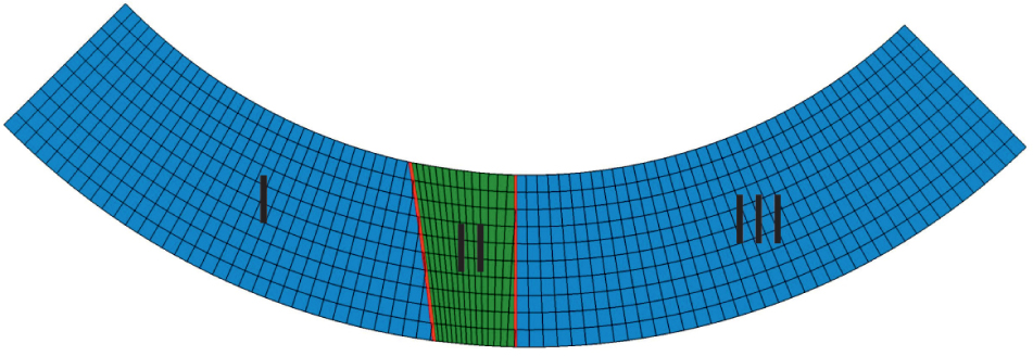
Illustrative figure of tooth side of globoidal worm wheel with marked region I, II, III.
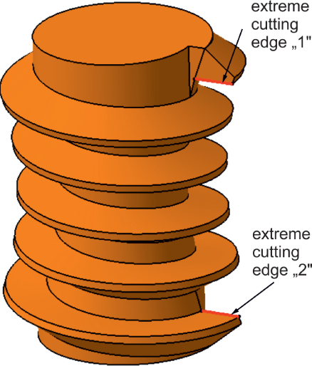
Illustrative figure of tool model with marked extreme cutting edges.
The condition of existence of an envelope is represented by the equation of meshing:
where:
n (nx, ny,nz)- normal vector to the surface,
v (vx, Vy, Vz)- tangent vector.
Relationship between rotation of worm wheel
The developed form of homogenous matrix
The normal vector
where: L2′1′ – is the matrix of transformation from 1′ do 2′.
L2′1′ is obtained by crossing out the last row and the last column of the homogeneous matrix of transformation (24).
In equation (25) the partial derivative of position vector
Tangent vector can be calculated based on kinematics of worm gear machining. Tangent vector is given by the following expression:
The derivative
After solving the eq. (28), for given parameters u the solutions set of p1 is obtained. Substituting the solutions to eq. (21) the lines of contact between worm and worm wheel in
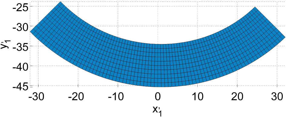
Contact lines shown in
Worm surface is in tangent with worm wheel surface at every instant of two lines. One contact line lies in the central plane of worm drive. It is constant and straight. The other contact line is curvilinear and is moving to the first on each worm wheel tooth being in mesh with worm. These lines generate that part of worm wheel, which is described as region II. Region II is generated as the envelope to the family of surface Σ1. This part of worm wheel
These lines are selected, which are not lying in the axial section of worm. Then the selected contact lines should be brought to the one tooth side of worm wheel, as shown as example in Fig. 8.

Region II presented in
In the developed algorithm contact lines are determined for one tooth side of worm wheel. The tool is set in the base position (in this position the extreme edge of the tool is in the central plane). For this purpose, by solving the equation (28) the rotation parameter
In the matrix
In the equation (31) in the matrix
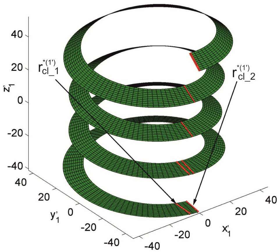
Region I and III is formed by a first cutting edge of worm hob cutter. It is equivalent with the extreme contact line
In the matrix
or
where:
In eq. (33) in the matrix

Surface generated by extreme cutting edge of the tool.
From the surface shown in Fig. 9 region I and III have to be separated. The two contact lines in the area of the extreme cutting edge of the tool are the boundaries of the regions (Fig. 7). For region I there is the contact line, which doesn’t lie in the axial plane of tool
The separated region I and III of the worm wheel tooth surface generated during machining through the extreme edge of the tool.
The algorithm for selecting the region I
where:
Equation (34) specifies the range of coordinates (i, j) of the table for region I. It can be expressed as:
where: i, j are satisfying the condition (34).
The algorithm for selecting the region III
where:
Equation (36) specifies the range of coordinates (i, j) of the table for region III. It can be expressed as
where: i, j are satisfying the condition (36).
The worm wheel tooth surface is generated by the combination of the regions I, II, III (Fig. 11):

The worm wheel tooth surface of globoidal worm drive generated by the tool with straight profile.
The worm wheel tooth profile in region I and III is straight and in the middle part – region II is concave.
6 Conclusions
The presented mathematical model can be used in practical application by designing new transmission gear. The double enveloping worm gear drive provides increased load capacity in comparison with the cylindrical worm gear drive. Because of this, it can replace the cylindrical worm gear in the gearbox, when the overall dimensions of the gear can’t be enlarged.
Final conclusions can be formulated by following points:
Presented mathematical model of globoidal worm drive with straight axial tooth profile shows that its determination is complex. The theory of gearing and gear generation mechanism was used.
The extreme cutting edge of worm hob has a considerable impact by generating the tooth side of worm wheel. It is circa 85% of tooth width of worm wheel.
The presented mathematical model of tooth flank of globoidal worm and worm wheel can be used for different analysis, like contact pattern, lubrication condition of the gear, etc.
The mathematical representation of tooth flank surface of hourglass worm and worm wheel can be helpful for generation CAD models, which can be used for FEM analysis.
References
[1] Dudas I., The theory and practice of worm gear drives, Penton Press, London, 2000.Search in Google Scholar
[2] Litvin F.L., Development of Gear Technology and Theory of Gearing. NASA, Levis Research Center, 1999.Search in Google Scholar
[3] Cone S.I., Globoidal hob, U.S. Pat. No. 2026215 A.Search in Google Scholar
[4] Cone S.I., Method of and apparatus for cutting worm gearing, U.S. Pat. No. 1885686 A.Search in Google Scholar
[5] Litvin F. L., Fuentes A., Gear Geometry and Applied Theory, Cambridge University Press, 2004.10.1017/CBO9780511547126Search in Google Scholar
[6] AGMA 6135 – A02, Design, Rating and Application of Industrial Globoidal Wormgearing (Metric Edition), American National Standard, 2002.Search in Google Scholar
[7] GOST 17696-89, Globoid gears. Calculation of geometry, 1989.Search in Google Scholar
[8] GOST 24438-80, Globoid gears. Basic worm and basic generating worm, 1980.Search in Google Scholar
[9] GOST 9369-77, Globoid gear pairs. Basic parameters, 1977.Search in Google Scholar
[10] Simon V., Double Enveloping Worm Gear Drive with Smooth Gear Tooth Surface, Proceedings, International Conference on Gearing, Zhengzhou, China, 1988, 191-194.Search in Google Scholar
[11] Simon V., A New Type of Ground Double Enveloping Worm Gear Drive, Proceedings, ASME 5th International Power Transmissions and Gearing Conference, Chicago, 1989, 281-288.Search in Google Scholar
[12] Simon V., Load Distribution in Double Enveloping Worm Gears, ASME Journal of Mechanical Design, 1993, 115, 496-501.10.1115/1.2919217Search in Google Scholar
[13] Simon V., Characteristics of a Modified Double Enveloping Worm Gear Drive, Proceedings, 6th International Power Transmission and Gearing Conference, Scottsdale, 1992, 73-79.10.1115/DETC1992-0010Search in Google Scholar
[14] Zhao Y., Meshing analysis for TA worm, In: Wenger P., Flores P., New Trends in Mechanism and Machine Science, Mechanism and Machine Science, Springer, 43, 2017, 13-20.10.1007/978-3-319-44156-6_2Search in Google Scholar
[15] Zhao Y., Novel methods for curvature analysis and their application to TA worm, Mechanism and Machine Theory, 2016, 97(3), 155-170.10.1016/j.mechmachtheory.2015.11.003Search in Google Scholar
[16] Mohan L. V., Shunmugam M. S., Geometrical aspects of double enveloping worm gear drive. Mechanism and Machine Theory, 2009, 44(11), 2053-2065.10.1016/j.mechmachtheory.2009.05.008Search in Google Scholar
[17] Buckingham E., Analytical Mechanics of Gears, Dover Publications Inc., New York, 1949.Search in Google Scholar
[18] Nieslony P., Krolczyk G.M., Zak K., Maruda R.W., Legutko S., Comparative assessment of the mechanical and electromagnetic surfaces of explosively clad Ti-steel plates after drilling process, Precision Engineering, 2017, 47, 104-110.10.1016/j.precisioneng.2016.07.011Search in Google Scholar
[19] Nieslony P., Krolczyk G.M., Wojciechowski S., Chudy R., Zak K., Maruda R.W. Surface quality and topographic inspection of variable compliance part after precise turning, Applied Surface Science, 2018, 434, 91-101, (in press), 10.1016/j.apsusc.2017.10.158.Search in Google Scholar
[20] Maruda R., Legutko S., Krolczyk G., Raos P., Influence of cooling conditions on the machining process under MQCL and MQL conditions, Tehnicki Vjesnik – Technical Gazette, 2015, 22 (4), 965-970.10.17559/TV-20140919143415Search in Google Scholar
[21] Krolczyk G., Raos P., Legutko S. Experimental analysis of surface roughness and surface texture of machined and fused deposition modelled parts, Tehnički Vjesnik - Technical Gazette, 2014, 21(1), 217-221.10.2478/mms-2014-0060Search in Google Scholar
[22] Kornberger Z., Przekladnie slimakowe. Wydawnictwo WNT, Warszawa, 1973 (In Polish).Search in Google Scholar
© 2017 Piotr Połowniak and Mariusz Sobolak
This work is licensed under the Creative Commons Attribution-NonCommercial-NoDerivatives 4.0 License.
Articles in the same Issue
- Regular Articles
- The Differential Pressure Signal De-noised by Domain Transform Combined with Wavelet Threshold
- Regular Articles
- Robot-operated quality control station based on the UTT method
- Regular Articles
- Regression Models and Fuzzy Logic Prediction of TBM Penetration Rate
- Regular Articles
- Numerical study of chemically reacting unsteady Casson fluid flow past a stretching surface with cross diffusion and thermal radiation
- Regular Articles
- Experimental comparison between R409A and R437A performance in a heat pump unit
- Regular Articles
- Rapid prediction of damage on a struck ship accounting for side impact scenario models
- Regular Articles
- Implementation of Non-Destructive Evaluation and Process Monitoring in DLP-based Additive Manufacturing
- Regular Articles
- Air purification in industrial plants producing automotive rubber components in terms of energy efficiency
- Regular Articles
- On cyclic yield strength in definition of limits for characterisation of fatigue and creep behaviour
- Regular Articles
- Development of an operation strategy for hydrogen production using solar PV energy based on fluid dynamic aspects
- Regular Articles
- An exponential-related function for decision-making in engineering and management
- Regular Articles
- Usability Prediction & Ranking of SDLC Models Using Fuzzy Hierarchical Usability Model
- Regular Articles
- Exact Soliton and Kink Solutions for New (3+1)-Dimensional Nonlinear Modified Equations of Wave Propagation
- Regular Articles
- Entropy generation analysis and effects of slip conditions on micropolar fluid flow due to a rotating disk
- Regular Articles
- Application of the mode-shape expansion based on model order reduction methods to a composite structure
- Regular Articles
- A Combinatory Index based Optimal Reallocation of Generators in the presence of SVC using Krill Herd Algorithm
- Regular Articles
- Quality assessment of compost prepared with municipal solid waste
- Regular Articles
- Influence of polymer fibers on rheological properties of cement mortars
- Regular Articles
- Degradation of flood embankments – Results of observation of the destruction mechanism and comparison with a numerical model
- Regular Articles
- Mechanical Design of Innovative Electromagnetic Linear Actuators for Marine Applications
- Regular Articles
- Influence of addition of calcium sulfate dihydrate on drying of autoclaved aerated concrete
- Regular Articles
- Analysis of Microstrip Line Fed Patch Antenna for Wireless Communications
- Regular Articles
- PEMFC for aeronautic applications: A review on the durability aspects
- Regular Articles
- Laser marking as environment technology
- Regular Articles
- Influence of grain size distribution on dynamic shear modulus of sands
- Regular Articles
- Field evaluation of reflective insulation in south east Asia
- Regular Articles
- Effects of different production technologies on mechanical and metallurgical properties of precious metal denture alloys
- Regular Articles
- Mathematical description of tooth flank surface of globoidal worm gear with straight axial tooth profile
- Regular Articles
- Earth-based construction material field tests characterization in the Alto Douro Wine Region
- Regular Articles
- Experimental and Mathematical Modeling for Prediction of Tool Wear on the Machining of Aluminium 6061 Alloy by High Speed Steel Tools
- Special Issue on Current Topics, Trends and Applications in Logistics
- 10.1515/eng-2017-0001
- Special Issue on Current Topics, Trends and Applications in Logistics
- The Methodology of Selecting the Transport Mode for Companies on the Slovak Transport Market
- Special Issue on Current Topics, Trends and Applications in Logistics
- Determinants of Distribution Logistics in the Construction Industry
- Special Issue on Current Topics, Trends and Applications in Logistics
- Management of Customer Service in Terms of Logistics Information Systems
- Special Issue on Current Topics, Trends and Applications in Logistics
- The Use of Simulation Models in Solving the Problems of Merging two Plants of the Company
- Special Issue on Current Topics, Trends and Applications in Logistics
- Applying the Heuristic to the Risk Assessment within the Automotive Industry Supply Chain
- Special Issue on Current Topics, Trends and Applications in Logistics
- Modeling the Supply Process Using the Application of Selected Methods of Operational Analysis
- Special Issue on Current Topics, Trends and Applications in Logistics
- Possibilities of Using Transport Terminals in South Bohemian Region
- Special Issue on Current Topics, Trends and Applications in Logistics
- Comparison of the Temperature Conditions in the Transport of Perishable Foodstuff
- Special Issue on Current Topics, Trends and Applications in Logistics
- E-commerce and its Impact on Logistics Requirements
- Topical Issue Modern Manufacturing Technologies
- Wear-dependent specific coefficients in a mechanistic model for turning of nickel-based superalloy with ceramic tools
- Topical Issue Modern Manufacturing Technologies
- Effects of cutting parameters on machinability characteristics of Ni-based superalloys: a review
- Topical Issue Desktop Grids for High Performance Computing
- Task Scheduling in Desktop Grids: Open Problems
- Topical Issue Desktop Grids for High Performance Computing
- A Volunteer Computing Project for Solving Geoacoustic Inversion Problems
- Topical Issue Desktop Grids for High Performance Computing
- Improving “tail” computations in a BOINC-based Desktop Grid
- Topical Issue Desktop Grids for High Performance Computing
- LHC@Home: a BOINC-based volunteer computing infrastructure for physics studies at CERN
- Topical Issue Desktop Grids for High Performance Computing
- Comparison of Decisions Quality of Heuristic Methods with Limited Depth-First Search Techniques in the Graph Shortest Path Problem
- Topical Issue Desktop Grids for High Performance Computing
- Using Volunteer Computing to Study Some Features of Diagonal Latin Squares
- Topical Issue on Mathematical Modelling in Applied Sciences, II
- A polynomial algorithm for packing unit squares in a hypograph of a piecewise linear function
- Topical Issue on Mathematical Modelling in Applied Sciences, II
- Numerical Validation of Chemical Compositional Model for Wettability Alteration Processes
- Topical Issue on Mathematical Modelling in Applied Sciences, II
- Innovative intelligent technology of distance learning for visually impaired people
- Topical Issue on Mathematical Modelling in Applied Sciences, II
- Implementation and verification of global optimization benchmark problems
- Topical Issue on Mathematical Modelling in Applied Sciences, II
- On a program manifold’s stability of one contour automatic control systems
- Topical Issue on Mathematical Modelling in Applied Sciences, II
- Multi-agent grid system Agent-GRID with dynamic load balancing of cluster nodes