Artificial intelligence enabled microgrid power generation prediction

3.1 System model

To have a better understanding of the PV electricity generation process, figuring out the PV system structure and setting up configurations of PV panels are very important.

Sandia National Laboratories, which operates under the U.S. Department of Energy has published one of the related mathematical models is: the Plane of Array (POA) Model [30], which figures out the mathematical relation between the solar energy that PV panels absorbed, and the solar radiation is necessary. POA represents the PV panel surface and the irradiance cast on POA can be calculated by equation (1) [30].

in which three main components of the POA irradiance, E b is the POA beam component, E g is the POA ground reflect component, E d is POA sky diffuse component [30]. The overall solar irradiance reflected on the solar panel is the summation of the irradiance from direct sun irradiance, irradiance reflected from the ground, and irradiance diffused from the sky.

Moreover, the POA beam component is decided by Direct Normal Irradiance and the angle between the sun rays and the PV panel, which is determined by not only the solar azimuth, and zenith angles, but also the tilt, azimuth angles of the PV panel [31], in which DNI denotes direct normal irradiance, AOI denotes angle of incidence.

POA formula’s second component ground reflected irradiance can be calculated as the following equation. The main affected variables include global horizontal irradiance GHI, the ground surface reflectivity, which is also called ground albedo ρ , and the tilt angle of the PV panel mentioned in the PV structure section θ T [32]. Here, ρ denotes albedo, which is highly dependent on the ground color and material. When the surface is dark, ρ ≈ 0 ; when the surface is bright white, ρ ≈ 1 [33].

Sky diffuse irradiance has several different theory models, like isotropic sky diffuse model [34], Hay and Davies Sky Diffuse Model [35], Reindl Sky Diffuse Model [36], and Perez Sky Diffuse Model [37]. This report used the simple isotropic model to demonstrate sky diffuse [34,38].

Also, the ground horizontal irradiance (GHI) could be calculated by the diffuse horizontal irradiance (DHI), direct normal irradiance (DNI), and solar zenith angles θ Z following the equation (5)  [39]. In [40], the author mentioned that the DHI value is around 10–20% of GHI value on a sunny day, however, when encountering a cloudy day, the DHI value is almost equal to the GHI value.

As a result, the irradiance reflected on the PV panel in total could be calculated by putting equations (2), (3), (4) into equation (1)

in which the DNI can be derived from an absolute cavity radiometer; POA can be obtained by a pyranometer; AOI is mainly determined by solar azimuth θ A , solar zenith θ Z , and surface tilt angle θ T . The albedo parameter ρ as mentioned before, denotes the reflectivity of the ground surface [31–33]. In practice, parameters θ A , and θ Z are related to the sun’s position which is changed by date (time-related features). The tilt angle of the surface of PV panel θ T will be dynamic as well if it is a solar tracking rack rather than a steady PV panel.

To provide an intuitive feeling of three components: beam, ground reflect, and sky diffuse, the numeric values were provided to understand each component’s contributions to the POA model. The daily average global, beam, and diffuse irradiance component measurements in Kimberly, Idaho are 413, 481, and 132 W/m 2 , respectively [41]. In another research [42], the author provided DNI, GHI, and DHI measurement values in Doha, Qatar, which are 200.4, 225.2, and 94.7 W/m 2 , respectively, among half-year records.

To sum up, despite solar irradiance related weather factors DNI and DHI, there are some time-related features ( θ A , θ Z ), some weather-related features (cloud cover, temperature), and other external environment features ( ρ , θ T ) that existed in the PV generation model.

3.2 Predictive framework

The PV generation forecasting process will follow the steps in the flow chart. After obtaining the original PV generation data and related weather data, two datasets will first be preprocessed to get rid of the missing and wrong data and aligned by their timestamps afterward. Then, the processed time, PV generation data, and weather data will be fed into the XGBoost model to decide on the most important and effective input features for the proposed resilient model. Finally, SARIMA and long short-term memory network (LSTM) algorithms are used predict PV generation in the short term, comparing models’ performance under different input features. The predictive framework flowchart is illustrated in Figure 1.

Figure 1

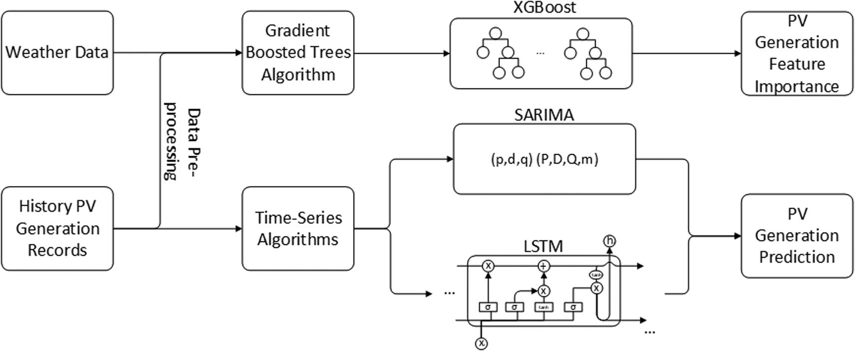
PV power generation prediction framework flowchart.

3.3 XGBoost model

CART tree algorithm, which is short for classical classification and regression tree, is the title for both trees: Classification tree (the prediction results are types) and regression tree (the prediction results are numeral). CART tree is a nonparametric decision tree algorithm [43]. CART algorithm first puts the input dataset in the root node, splits sub-nodes from the root node according to the attribute, and decides the best homogeneity for the threshold; the splitting process keeps going until a pure subset or meets the maximum node depth. The final node called leaf node is the one who holds the decision [8,43]. This whole iteration process will provide the relative best-fit model.

The eXtreme gradient boosting (XGBoost) is a supervised, improved gradient-boosted trees algorithm, which is integrated by many CART trees. The XGBoost’s regularized objective function L ( ϕ ) includes training loss and regularization term [44].

The differentiable convex training loss ( L ) measures the predictive ability of the model by comparing the difference between prediction value y i ˆ and measurement value y i . f k denotes independent tree structure and leaf weights.

Regularization term ( Ω ) refers to the part that controls the model complexity that prevents the model from overfitting, which can be demonstrated as follows [44,45]:

where Ω defines the complexity of the tree f ; λ determines the strength of the regularization; γ is a penalise nodes constant, when it is greater than 1; and T denotes the number of leaves in the tree.

The XGBoost algorithm optimizes the function by keep adding new trees to simulate the residuals from the last prediction rather than using methods in Euclidean space [43,44]. The purpose of the model is to find f p value to optimise the objective function by searching the smallest score [44]. In dataset D = ( x i , y i ) , ( x i denotes examples, and y i denotes features), the objective function L ( p ) can be presented as as follows [43,44]:

where y ˆ i ( p ) refers to the prediction value on p th iteration of i th instance [44].

To simplify the objective function, the constant terms ∑ i = 1 n l ( y i , y ˆ ( p − 1 ) ) could be removed [44]. By applying one of the common training loss functions mean squared error (MSE) and regularization term Ω ( f p ) , the objective function can be simplified as follows [43]:

After the process of second-order approximation, this objective equation (9) sums the first and second input gradient statistics g i and h i up together as G j and H j and then calculates the score according to the formula, which indicates the quality of the tree structure [43].

This article used the XGBoost model purely for time-series PV data predicting, which separates the various time factors (like months, weeks, days, and hours) from PV generation data and stores them in a tree. Finally, predict future PV generation based on the summarized time features relationship.

3.4 Seasonal ARIMA model

Autoregressive integrated moving average (ARIMA) is one of the effective univariate time series algorithms. As an extended version, seasonal autoregressive integrated moving average (SARIMA) algorithm supports both autoregressive and moving average functions [46], which means SARIMA would identify seasonal changing input data and make better predictions compared to ARIMA. Seasonal changing data refer to the training data value changes due to seasonal factors. Accordingly, we use the SARIMA model to train and predict the PV generation value. The SARIMA model can be formed as SARIMA ( ( p , d , q ) , ( P , D , Q , m ) ) in which ( p , d , q ) represents the nonseasonal feature from the data; ( P , D , Q , m ) represents the seasonal feature. In more detail, p represents trend auto-regression order; d represents trend difference order; q moving average order; P represents seasonal auto-regressive order; D represents seasonal difference order; Q represents seasonal moving average order; and m represents the number of time steps for a seasonal period [46]. The SARIMA model can be formulated as equation (11)

where y t denotes the value of the time series at time t , ϕ denotes the coefficients of the auto-regressive, θ denotes coefficients of the auto regressive forecast errors; ε denotes the moving average forecast error; η denotes coefficients of seasonal forecast errors; and ω denotes coefficients of seasonal auto regressive. The enumeration function was used to list all ( p , d , q ) and ( P , D , Q , m ) combinations to look for the best model fit, which is judged by the lowest Akaike information criterion (AIC) value [47].

3.5 Long short-term memory network (LSTM)

LSTM is one type of the RNN (recurrent neural network) especially overcome exploding and vanishing gradient problems during long-term dependencies, which has recurrent neurons to process the input data through the activation and formulate an output to the next neuron [48]. The LSTM is good at solving the sequence problems because of the feedforward network from the last training [49], which no longer suffers from Simple Recurrent Networks [50]. A typical vanilla LSTM model architecture can be demonstrated as multiple memory blocks shown in Figure 2 [48,51].

Figure 2

LSTM memory block demonstration.

In this special memory block, there are three essential multiplicative units: input gate, output gate, and forget gate, which always use sigmoid as their nonlinear activation function [48]. This memory block first takes previous memory c t − 1 , output h t − 1 , and input signal X t as input to feed through input gate [48,52–54].

Second, in forget gate, the memory block decides what information will be forgotten based on the input signal X t , memory c t − 1 , and output h t − 1 from the previous block [48,52–54].

Third step is generating output combining input signal X t , memory c t − 1 , and output h t − 1 from last iteration [48,52–54].

This memory block iteration will carry on when more input data has been fed through the LSTM model. LSTM networks there would be another loop in the model, which will provide the feedback value as an input vector from an output of the network to the input of the network [48].

4.1 Data preparation

The quality of the input dataset may affect the training model’s performance and accuracy [55], which means two data preprocessing steps: data cleaning and filtering missing data are necessary [56]. After the data preprocessing steps, the data normalized step is required to reduce the noise and normalize the dataset.

In this work, for the XGBoost, SARIMA, and LSTM algorithms, 1 year London area’s PV electricity generation record from Sheffield open-source PV live data (London area) and weather data were from MIDAS UK open weather data^[1]. The data were from the Heathrow station, and both of the datasets (PV and weather) start from 2020/01/01 to 2020/12/27, recording in every 60 min. Due to the synchronization failure and misoperations, there are some repeated data or vacant data. In the data preprocessing step, we removed the repeat data according to the date and time, and then left the vacant records (NaN) as noise. As a result, the PV generation dataset has in total of 8657 records after the preprocessing step.

The PV generation data itself are recorded in Megawatts, and hourly generation records can reach up to thousands of megawatts, sometimes even more than 5,000 MW. However, at night, due to lack of solar irradiance, the PV generation equals 0 mostly. The large periodical difference in the dataset will not benefit the learning process, which means that the data normalization process is necessary as well. MinMaxScaler function was used to scale all the PV generation data under [0,1] scale. The weather data air temperature are stored in the degree Celsius; the global solar irradiance mount is stored in kJ/m².

The Pearson correlation coefficient model was used to analyze the associations behind the feature data. It is a normalization evaluation method of the covariance of two features, which reviews the strength and direction of linear correlation between them [57]. On the one hand, the various weather data were studied including time-related features’ correlations with PV electricity generation, which can be illustrated in Figure 3.

Figure 3

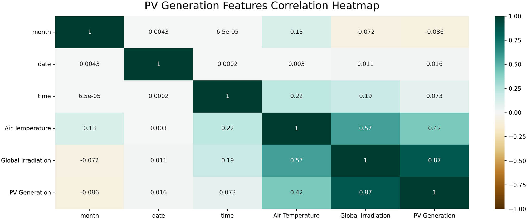
Heatmap of PV generation features correlation.

By analyzing the correlation between features from the dataset, we can see that pure time features like hours, date, and month do not have much correlation with hourly PV generation because their correlation values with PV generation are close to 0. However, previous records of global irradiance and air temperature have a very high correlation to the next hour’s PV generation, which means they could be the main features that contribute to the prediction model.

On the other hand, the correlation between history PV generation (24 h before) and current PV generation was also studied. Because the POA model is very complex and contains various times, weather, and other features, we cannot easily have access to all of them. In contrast, the previous PV generation data are the accurate value simulated by all the factors. The correlation heatmap between history and current PV generation value is shown in Figure 4, where P_24 refers to PV generation from 24 h ago, and P_0 refers to the PV generation in the future 1 h, which needs to be predicted.

Figure 4

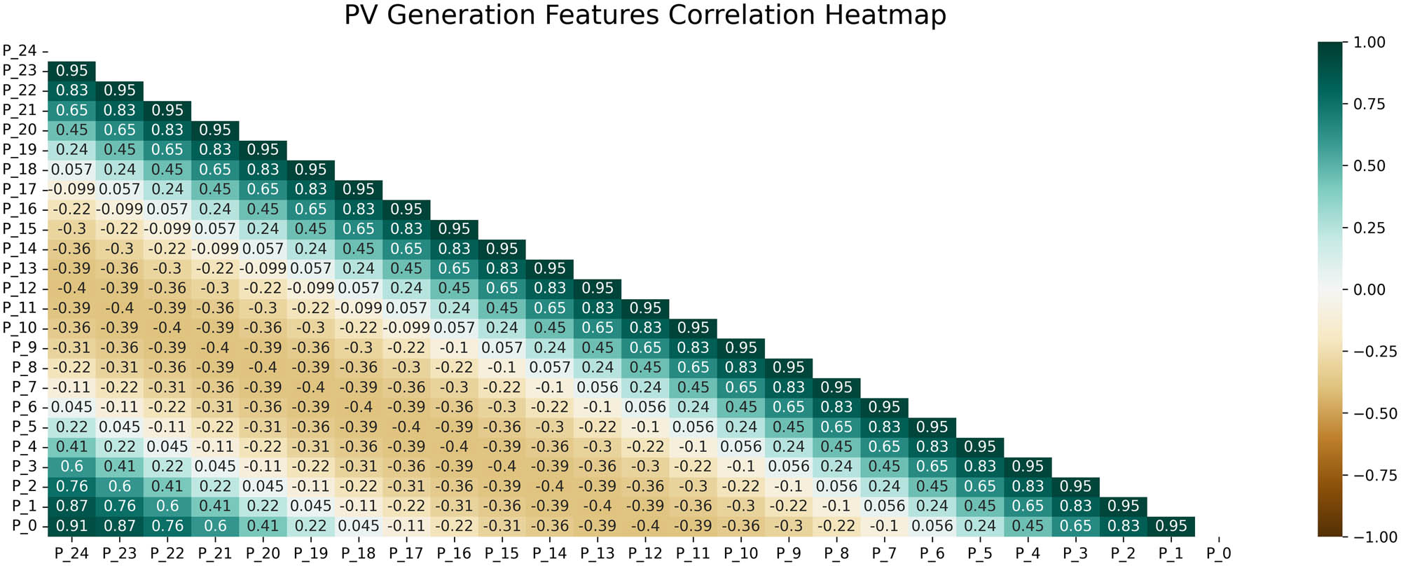
Heatmap of PV generation features correlation.

From Figure 4, P_1 to P_3 (previous 3 h) and P_21 to P_24 (yesterday 3 h after) PV generation have a high correlation (above 0.6) to the future 1 h PV generation prediction. The other hours of PV generation also have some associations with the future PV generation data.

To sum up, we used a total of 8752 records (from 2020/01/01 0:00 to 2020/12/21 23:00) to train the XGBoost model. The dataset is developed in six columns: month, date, time, air temperature, global irradiance, and PV generation. By applying different feature combinations to the algorithms to receive a high-performance model that requires minimum data. The testing dataset will be from 6 days of records (from 2020/12/22 0:00 to 2020/12/27 23:00).

4.2 XGBoost

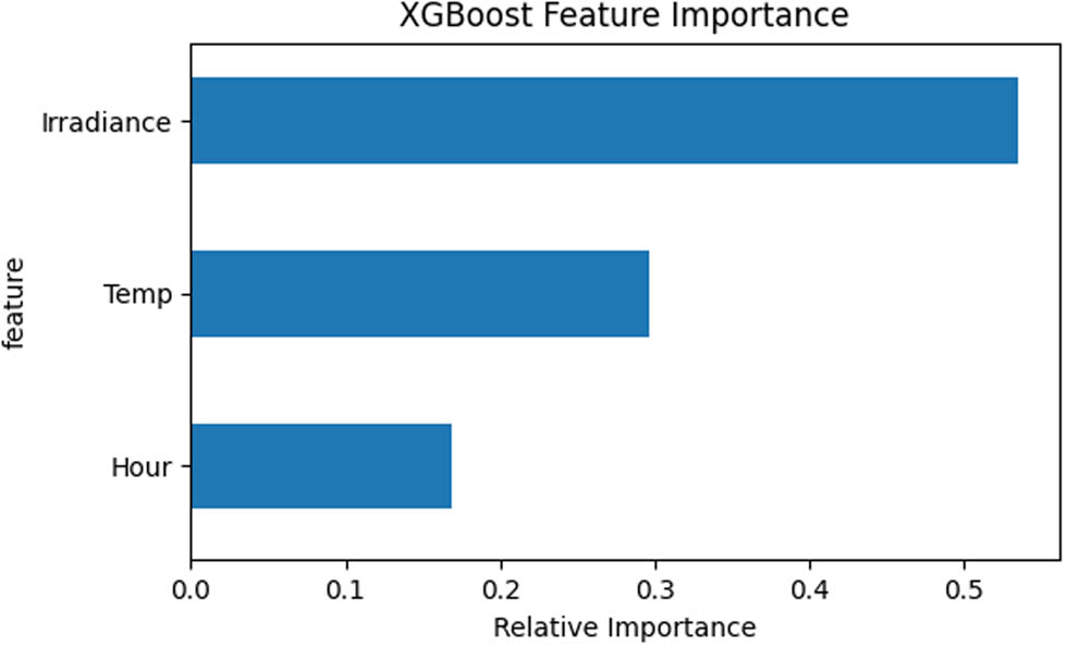
To find the ideal prediction model, this work first used the XGBoost model to verify and analyze the hypothesis we concluded from the first Pearson correlation model that solar irradiance and air temperature are the core features to predict short-term PV generation. The XGBoost model predicts future PV generation based on the previous 1 h weather data and the time data without the data normalization process to keep the original data features. As a result, PV generation prediction uses megawatts as its measurement unit. PV generation data’s relationships in the XGBoost model among different features can be illustrated in Figure 5.

Figure 5

XGBoost time features analysis in PV generation data.

XGBoost feature importances function utilizes F score that indicates each feature’s percentage weight over the weights of all features. As Figure 5 shows, in XGBoost, solar irradiance has over 50% importance and air temperature has around 30% importance for this dataset.

For the hyperparameter optimization part, we still used the grid search method to automatically test the best fit of parameters for the XGBoost model. The XGBoost prediction model fit is shown in Figure 6, which is an XGBoost 1 h ahead prediction model using previous hours, solar irradiance, and air temperature as the training dataset.

Figure 6

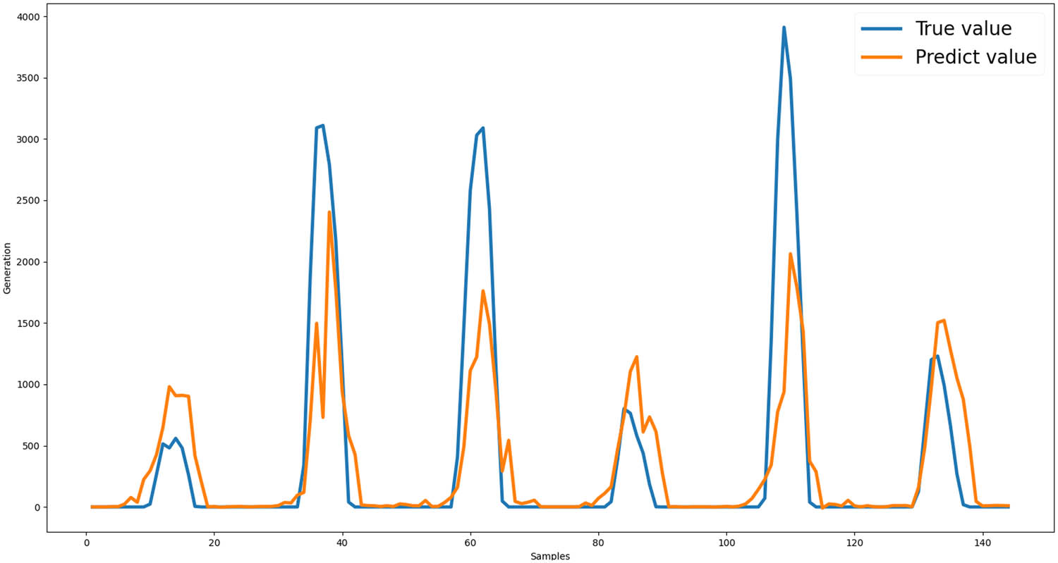
XGBoost PV generation prediction.

From the figure, we can see that the XGBoost model only using previous one-hour solar irradiance, air temperature, and hours time data shows low prediction accuracy on the summit PV generation of the day. The average R 2 score is around 0.7; the root mean squared error (RMSE) value is around 467 (MW). This model’s performance is not very well for just using previous weather data and time data as its input. As a result, we decided to use previous PV generation data as input instead of using previous solar irradiance and air temperature. Because previous weather data are more related to previous PV generation instead of PV generation in the future. Also, previous PV generation is always accurate and more related to the predicting panel (containing more complex features) compared to the local weather data.

4.3 SARIMA

To confirm the correlation between history and current PV generation, we utilized the time-series algorithm SARIMA to predict the current generation value using the previous generation value analyzed by date and time. The auto-regression part of the SARIMA model measures the dependency by past observations, which will use the previous 8,700 data records as the training dataset. Also, from observation of the PV generation value, the value repeats in a similar tendency loop for 24 h of solar movement, which means the PV generation value can be set in a 24 h (24 records) seasonal period in a SARIMA model. The test data will be 6 days starting from 2020/12/22 to 2020/12/27.

Our goal is to find the best-fit value for SARIMA ( p , d , q ) ( P , D , Q , m ) to optimize the interest metric. We used the hyperparameter optimization method, Grid Search, to generate and test different combinations of variables p , d , q , and then evaluate the model accuracy by comparing their AIC value. AIC value is a common model selection theory, which will gradually minimize the mean squared error of prediction to find the best fit [58]. Normally, the lower AIC value is considered to be a better model fit.

After the grid search process, the best hyperparameters that fit the SARIMA model are ( 1 , 1 , 1 ) ( 1 , 1 , 1 , 24 ) with the lowest AIC score of 262.36. The SARIMA short-term PV prediction can be illustrated in Figure 7.

Figure 7

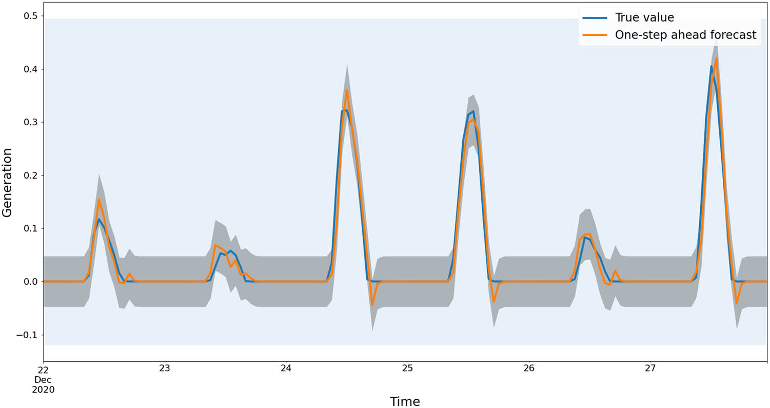
SARIMA PV generation prediction.

The SARIMA model’s coefficients are listed in Table 1, where ar.L1 and ma.L1 rows denote autoregressive (AR) and moving average (MA) coefficients for the nonseasonal component of the model, respectively. Similarly, “ar.S.L24” and “ma.S.L24” denote the AR and MA coefficients, respectively, the seasonal component of the model, where the seasonality is specified as 24 h. The sigma2 (sigma square) column denotes the variance of residual values; the coef column denotes weights of each feature; the std err column denotes standard error. The significance of each coefficient is assessed using the z -test, with the associated p -values provided in the “ P > ∣ z ∣ ” column. A p -value less than the conventional threshold of 0.05 indicates that the corresponding coefficient is statistically significant, suggesting that it has a significant association with the predicted PV generation.

As Figure 7 shows, the SARIMA model has relatively high accuracy and confidence (average mean absolute error [MAE], is around 0.0097, average RMSE is around 0.0196) on short-term PV generation predicting. The grey shadow in the figure is the confidence bounds of the prediction model, which refers to the uncertainty of each step of prediction. However, we can still see that there are imprecise predictions during the end of the day and the summit generation in a day.

4.4 LSTM

The LSTM model was first used to conduct one-step ahead PV generation prediction as a comparison group with the SARIMA model. We set the look-back window as 24 (last 1-day records) so that the LSTM algorithm will take previous 1-day records to predict the value. The LSTM model contains 50 neurons, mean square error as loss function, and the adam optimizer. LSTM model’s average score ( R 2 ) is around 0.96, and average RMSE is around 0.2. The best LSTM one-step ahead model we conduct can be illustrated in Figure 8.

Figure 8

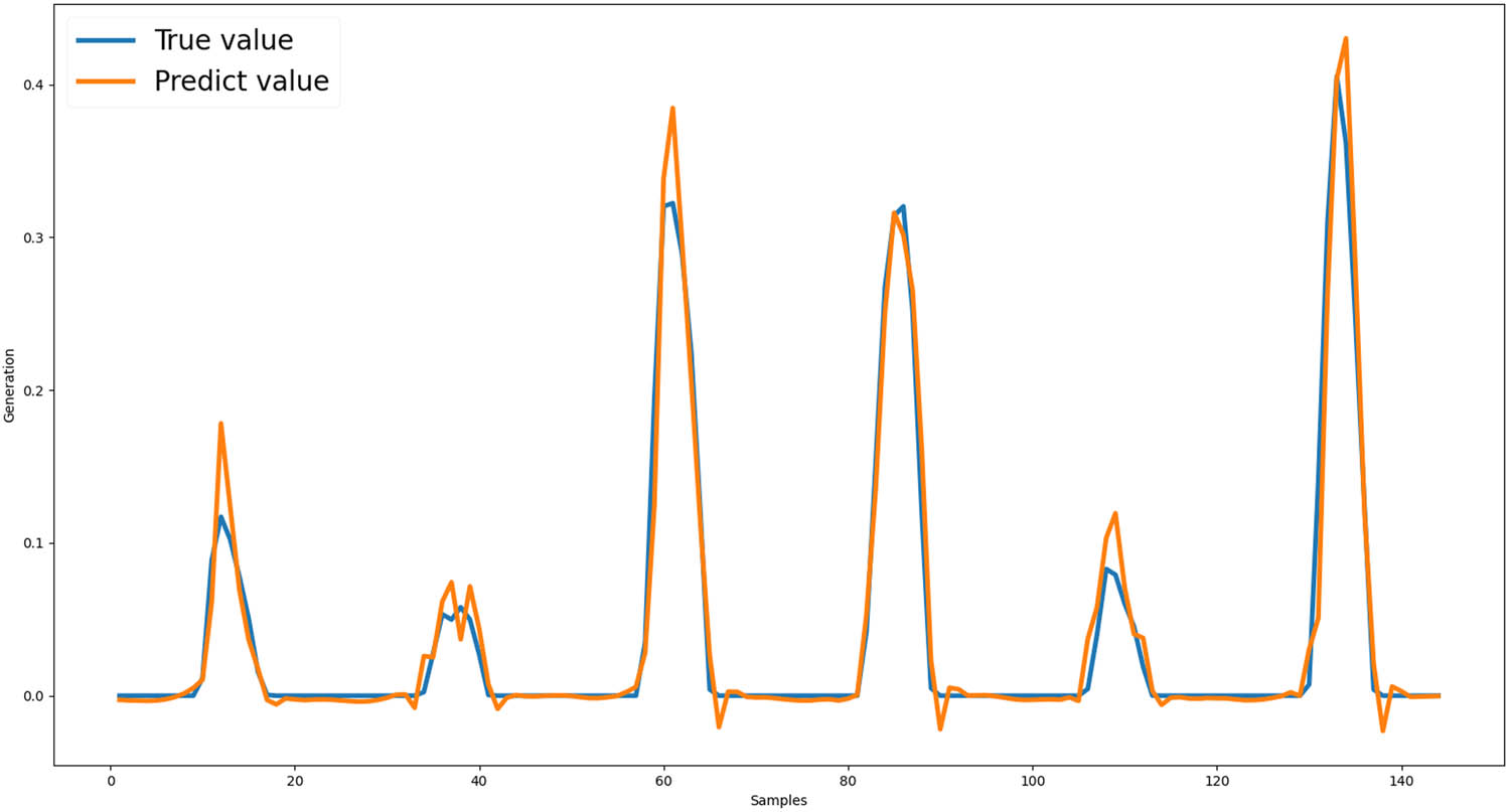
LSTM PV generation prediction.

LSTM 1 h ahead short-term prediction using 24 h history records has a relatively good performance, even though sometimes it is still limited in predicting the summit PV generation value of the day and some other turning points. Then, to find a resilient and high-performance model, we also added the weather data (solar irradiance and air temperature) and tested other look-back window sizes on the LSTM model to reduce the input feature amount. Different input feature combinations’ requirements and performance are listed in Table 1.

4.5 Result comparison

We researched the time-series PV generation algorithms SARIMA and LSTM, which use previous PV generation data to predict future generations. We used four common evaluation methods R 2 score ( R 2 ), MAE, MSE, and RMSE.

R 2 score, which also means coefficient of determination, describes the accuracy of dependent variable changes according to the prediction of independent variables. In other words, it explains how well the data fit the model and R 2 = 1 represents the perfect fit. y i denotes the true value of the dataset, y ˆ i denotes the predicted value, and y ¯ i denotes the mean value.

MAE represents the average of absolute residuals between the prediction and true value, which can be calculated as follows:

MSE measures the average square errors between predicted and true values. Compared to MAE, it measures the variance of residuals rather than the average of residuals. It can be calculated as follows:

RMSE is the square root of the MSE value, which measures the standard deviation of residuals and can be calculated as follows:

In the algorithm results comparison table, * denotes the dataset with normalization; ‘denotes to the dataset with weather data (solar irradiance and air temperature). The number after LSTM denotes the look-back number. For example, LSTM*’ 5 refers to the LSTM model utilizing the normalization dataset and weather data, using the previous 5 h of PV generation data as a look-back window. For each of the models, we used an average score among 20 times model fitting (Table 2).

From the comparison, we can see that the LSTM model using 24 history PV generation records and weather data does have excellent performance (average R 2 score can reach 0.9563, and average RMSE is around 0.0195). However, various input features reduce the resilience and robustness of the model. When there are not that much PV generation data available or some of them are not accurate because of cyber attacks, the model will not perform or make an accurate prediction in that circumstance. Instead, we studied various LSTM models that require minimum input data to guarantee the model’s resilience. In the table, LSTM models only use the previous two records and three records of PV generation data as input and have relatively high performance (with an average R 2 score of around 0.90 and an average RMSE score is around 0.026).

However, when previous solar irradiance, air temperature, or other weather data are available combined with previous PV generation data, using multivariables LSTM algorithms will have a slightly better performance in short-term prediction (by comparing LSTM*’ models with LSTM* models).

References

[1] H. Kanchev, D. Lu, F. Colas, V. Lazarov, and B. Francois, “Energy management and operational planning of a microgrid with a pv-based active generator for smart grid applications,” IEEE Transactions on Industrial Electronics, vol. 58, no. 10, pp. 4583–4592, 2011. 10.1109/TIE.2011.2119451Suche in Google Scholar
[2] U. N. D. Programme, World Energy Assessment: Energy and the Challenge of Sustainability, 1st ed., New York, NY 10017: United Nations Development Programme, 2000. Suche in Google Scholar
[3] A. Detollenaere and G. Masson, Snapshot of global PV markets 2022 task 1 strategic PV analysis and outreach, IEA PVPS, Paris, France, pp. 8–10, 2022. Suche in Google Scholar
[4] N. M. Haegel, R. Margolis, T. Buonassisi, D. Feldman, A. Froitzheim, R. Garabedian, et al., “Terawatt-scale photovoltaics: Trajectories and challenges,” Science, vol. 356, no. 6334, pp. 141–143, 2017. 10.1126/science.aal1288Suche in Google Scholar PubMed
[5] R. Cioffi, M. Travaglioni, G. Piscitelli, A. Petrillo, and F. De Felice, “Artificial intelligence and machine learning applications in smart production: Progress, trends, and directions,” Sustainability vol. 12, no. 2, pp. 492–518, 2020. https://www.mdpi.com/2071-1050/12/2/492. 10.3390/su12020492Suche in Google Scholar
[6] A. D. Martin, J. M. Cano, J. F. A. Silva, and J. R. Vázquez, “Backstepping control of smart grid-connected distributed photovoltaic power supplies for telecom equipment,” IEEE Transactions on Energy Conversion, vol. 30, no. 4, pp. 1496–1504, 2015. 10.1109/TEC.2015.2431613Suche in Google Scholar
[7] G. G. Kim, J. H. Choi, S. Y. Park, B. G. Bhang, W. J. Nam, H. L. Cha, et al. “Prediction model for PV performance with correlation analysis of environmental variables,” IEEE Journal of Photovoltaics, vol. 9, no. 3, pp. 832–841, 2019. 10.1109/JPHOTOV.2019.2898521Suche in Google Scholar
[8] S. Ferlito, G. Adinolfi, and G. Graditi, “Comparative analysis of data-driven methods online and offline trained to the forecasting of grid-connected photovoltaic plant production,” Applied Energy, vol. 205, pp. 116–129, 2017. 10.1016/j.apenergy.2017.07.124Suche in Google Scholar
[9] M. N. Akhter, S. Mekhilef, H. Mokhlis, and N. Mohamed Shah, “Review on forecasting of photovoltaic power generation based on machine learning and metaheuristic techniques,” IET Renewable Power Generation, vol. 13, no. 7, pp. 1009–1023, 2019. 10.1049/iet-rpg.2018.5649Suche in Google Scholar
[10] G. Li, S. Xie, B. Wang, J. Xin, Y. Li, and S. Du, “Photovoltaic power forecasting with a hybrid deep learning approach,” IEEE Access, vol. 8, pp. 175871–175880, 2020. 10.1109/ACCESS.2020.3025860Suche in Google Scholar
[11] M. Massaoudi, H. Abu-Rub, S. S. Refaat, I. Chihi, and F. S. Oueslati, “Deep learning in smart grid technology: A review of recent advancements and future prospects,” IEEE Access, vol. 9, pp. 54558–54578, 2021. 10.1109/ACCESS.2021.3071269Suche in Google Scholar
[12] R. Bessa, A. Trindade, C. S. Silva, and V. Miranda, “Probabilistic solar power forecasting in smart grids using distributed information,” International Journal of Electrical Power and Energy Systems, vol. 72, pp. 16–23, 2015. 10.1016/j.ijepes.2015.02.006Suche in Google Scholar
[13] C. Gouveia, D. Rua, F. Soares, C. Moreira, P. Matos, and J. P. Lopes, “Development and implementation of portuguese smart distribution system,” Electric Power Systems Research, vol. 120, pp. 150–162, 2015. 10.1016/j.epsr.2014.06.004Suche in Google Scholar
[14] N. Gowtham, V. Prema, M. F. Elmorshedy, M. Bhaskar, and D. J. Almakhles, “A power aware long short-term memory with deep brief network based microgrid framework to maintain sustainable energy management and load balancing,” Distributed Generation & Alternative, Energy Journal, pp. 1–26, 2024. 10.13052/dgaej2156-3306.3911Suche in Google Scholar
[15] R. Abdulkader, H. M. Ghanimi, P. Dadheech, M. Alharbi, W. El-Shafai, M. M. Fouda, et al., “Soft computing in smart grid with decentralized generation and renewable energy storage system planning,” Energies, vol. 16, no. 6, p. 2655, 2023. 10.3390/en16062655Suche in Google Scholar
[16] A. Rajagopalan, D. Swaminathan, M. Alharbi, S. Sengan, O. D. Montoya, W. El-Shafai, et al., “Modernized planning of smart grid based on distributed power generations and energy storage systems using soft computing methods,” Energies, vol. 15, no. 23, p. 8889. 2022. https://www.mdpi.com/1996-1073/15/23/8889. 10.3390/en15238889Suche in Google Scholar
[17] O. A. Omitaomu and H. Niu, “Artificial intelligence techniques in smart grid: A survey,” Smart Cities, vol. 4, no. 2, p. 548–568, 2021. 10.3390/smartcities4020029Suche in Google Scholar
[18] M. Pérez-Ortiz, S. Jiménez-Fernández, P. A. Gutiérrez, E. Alexandre, C. Hervás-Martínez, and S. Salcedo-Sanz, “A review of classification problems and algorithms in renewable energy applications,” Energies, vol. 9, no. 8, p. 607, 2016. https://www.mdpi.com/1996-1073/9/8/607. 10.3390/en9080607Suche in Google Scholar
[19] T. Ma, H. Yang, and L. Lu, “Solar photovoltaic system modeling and performance prediction,” Renewable and Sustainable Energy Reviews, vol. 36, pp. 304–315, 2014. 10.1016/j.rser.2014.04.057Suche in Google Scholar
[20] B. Bhandari, S. R. Poudel, K.-T. Lee, and S.-H. Ahn, “Mathematical modeling of hybrid renewable energy system: A review on small hydro-solar-wind power generation,” International Journal of Precision Engineering and Manufacturing-Green Tech, vol. 1, p. 157–173, 2014. 10.1007/s40684-014-0021-4Suche in Google Scholar
[21] S. I. Vagropoulos, G. I. Chouliaras, E. G. Kardakos, C. K. Simoglou, and A. G. Bakirtzis, “Comparison of sarimax, sarima, modified sarima and ann-based models for short-term pv generation forecasting,” in: 2016 IEEE International Energy Conference (ENERGYCON), 2016, pp. 1–6. 10.1109/ENERGYCON.2016.7514029Suche in Google Scholar
[22] A. Álvarez Gallegos, L. Fara, A. Diaconu, D. Craciunescu, and S. Fara, “Forecasting of energy production for photovoltaic systems based on ARIMA and ANN advanced models,” International Journal of Photoenergy, vol. 2021, pp. 1–19, 2021. 10.1155/2021/6777488Suche in Google Scholar
[23] S. K. Chow, E. W. Lee, and D. H. Li, “Short-term prediction of photovoltaic energy generation by intelligent approach,” Energy and Buildings, vol. 55, pp. 660–667, 2012. 10.1016/j.enbuild.2012.08.011Suche in Google Scholar
[24] L. A. Fernandez-Jimenez, A. Muñoz-Jimenez, A. Falces, M. Mendoza-Villena, E. Garcia-Garrido, P. M. Lara-Santillan, et al., “Short-term power forecasting system for photovoltaic plants,” Renewable Energy, vol. 44, pp. 311–317, 2012. 10.1016/j.renene.2012.01.108Suche in Google Scholar
[25] M. Mao, W. Gong, and L. Chang, “Short-term photovoltaic output forecasting model for economic dispatch of power system incorporating large-scale photovoltaic plant,” 2013 IEEE Energy Conversion Congress and Exposition, ECCE 2013, pp. 4540–4545, Sep 2013. 10.1109/ECCE.2013.6647308Suche in Google Scholar
[26] E. G. Kardakos, M. C. Alexiadis, S. I. Vagropoulos, C. K. Simoglou, P. N. Biskas, and A. G. Bakirtzis, “Application of time series and artificial neural network models in short-term forecasting of PV power generation,” in: 2013 48th International Universities’ Power Engineering Conference (UPEC), 2013, pp. 1–6. 10.1109/UPEC.2013.6714975Suche in Google Scholar
[27] M. Malvoni, M. G. De Giorgi, and P. M. Congedo, “Forecasting of pv power generation using weather input data–preprocessing techniques,” Energy Procedia, vol. 126, pp. 651–658, 2017. 10.1016/j.egypro.2017.08.293Suche in Google Scholar
[28] Y. Sun, V. Venugopal, and A. R. Brandt, “Convolutional neural network for short-term solar panel output prediction,” in: 2018 IEEE 7th World Conference on Photovoltaic Energy Conversion (WCPEC) (A Joint Conference of 45th IEEE PVSC, 28th PVSEC and 34th EU PVSEC), 2018, pp. 2357–2361. 10.1109/PVSC.2018.8547400Suche in Google Scholar
[29] T. Kim, W. Ko, and J. Kim, “Analysis and impact evaluation of missing data imputation in day-ahead PV generation forecasting,” Applied Sciences, vol. 9, no. 1, p. 204, 2019. 10.3390/app9010204Suche in Google Scholar
[30] Q. Sun, K. Lin, C. Si, Y. Xu, S. Li, and P. Gope, “A secure and anonymous communicate scheme over the internet of things,” ACM Transactions on Sensor Networks (TOSN), vol. 18, no. 3, pp. 1–21, 2022. 10.1145/3508392Suche in Google Scholar
[31] X. Wang, S. Li, and M. Iqbal, “Live power generation predictions via AI-driven resilient systems in smart microgrids,” IEEE Transactions on Consumer Electronics, 2024. 10.1109/TCE.2024.3371256Suche in Google Scholar
[32] Sandia National Laboratories, Poa ground reflected. https://pvpmc.sandia.gov/modeling-steps/1-weather-design-inputs/plane-of-array-poa-irradiance/calculating-poa-irradiance/poa-ground-reflected/. Suche in Google Scholar
[33] Y. Liu and S. Li, “A review of hybrid cyber threats modelling and detection using artificial intelligence in IIOT,” Computer Modeling in Engineering & Sciences, vol. 140, no. 2, 2024. 10.32604/cmes.2024.046473Suche in Google Scholar
[34] P. Loutzenhiser, H. Manz, C. Felsmann, P. Strachan, T. Frank, and G. Maxwell, “Empirical validation of models to compute solar irradiance on inclined surfaces for building energy simulation,” Solar Energy, vol. 81, no. 2, pp. 254–267, 2007. 10.1016/j.solener.2006.03.009Suche in Google Scholar
[35] J. E. Hay, “Calculating solar radiation for inclined surfaces: Practical approaches,” Renewable Energy, vol. 3, no. 4, pp. 373–380, 1993. 10.1016/0960-1481(93)90104-OSuche in Google Scholar
[36] D. Reindl, W. Beckman, and J. Duffie, “Evaluation of hourly tilted surface radiation models,” Solar Energy, vol. 45, no. 1, pp. 9–17, 1990. 10.1016/0038-092X(90)90061-GSuche in Google Scholar
[37] R. Perez, P. Ineichen, R. Seals, J. Michalsky, and R. Stewart, “Modeling daylight availability and irradiance components from direct and global irradiance,” Solar Energy, vol. 44, no. 5, pp. 271–289, 1990. 10.1016/0038-092X(90)90055-HSuche in Google Scholar
[38] M. Lave, W. Hayes, A. Pohl, and C. W. Hansen, “Evaluation of global horizontal irradiance to plane-of-array irradiance models at locations across the united states,” IEEE Journal of Photovoltaics, vol. 5, no. 2, pp. 597–606, 2015. 10.1109/JPHOTOV.2015.2392938Suche in Google Scholar
[39] Sandia National Laboratories, Global horizontal irradiance. https://pvpmc.sandia.gov/modeling-steps/1-weather-design-inputs/irradiance-and-insolation-2/global-horizontal-irradiance/. Suche in Google Scholar
[40] F. Vignola, GHI correlations with DHI and DNI and the effects of cloudiness on one-minute data, June 2012. Suche in Google Scholar
[41] F. Vignola, P. Harlan, R. Perez, and M. Kmiecik, “Analysis of satellite derived beam and global solar radiation data,” Solar Energy, vol. 81, no. 6, pp. 768–772, 2007. 10.1016/j.solener.2006.10.003Suche in Google Scholar
[42] D. Perez-Astudilloa, and D. Bachour, “DNI, GHI and DHI ground measurements in Doha, Qatar,” Energy Procedia, vol. 49, pp. 2398–2404, 2014. 10.1016/j.egypro.2014.03.254Suche in Google Scholar
[43] B. Dutta, A classification and regression tree (cart) algorithm, analytics steps, July 27 2021. [Online]. https://www.analyticssteps.com/blogs/classification-and-regression-tree-cart-algorithm. Suche in Google Scholar
[44] T. Chen and C. Guestrin, “Xgboost: A scalable tree boosting system,” in: Proceedings of the 22nd ACM SIGKDD International Conference on Knowledge Discovery and Data Mining, ser. KDD ’16, New York, NY, USA: Association for Computing Machinery, 2016, p. 785–794. [Online].https://doi.org/10.1145/2939672.2939785. Suche in Google Scholar
[45] xgboost developers, Xgboost tutorials, 2021. https://xgboost.readthedocs.io/en/stable/tutorials/model.html. Suche in Google Scholar
[46] J. Brownlee, A gentle introduction to sarima for time series forecasting in python, Aug, 21, 2019. [Online.] https://machinelearningmastery.com/sarima-for-time-series-forecasting-in-python/ Suche in Google Scholar
[47] R. J. Hyndman and G. Athanasopoulos, Forecasting: Principles and Practice, 2nd edition Melbourne, Australia. OTexts.com/fpp2, 2018. https://otexts.com/fpp2/seasonal-arima.html. 10.32614/CRAN.package.fpp2Suche in Google Scholar
[48] G. Van Houdt, C. Mosquera, and G. Nápoles, “A review on the long short-term memory model,” Artificial Intelligence Review, vol. 53, no. 8, pp. 1573–7462, 2020. 10.1007/s10462-020-09838-1Suche in Google Scholar
[49] J. Brownlee, “Long short-term memory networks with python,” English PDF format EBook, 2017 [Online]. Suche in Google Scholar
[50] K. Greff, R. K. Srivastava, J. Koutník, B. R. Steunebrink, and B. R. Schmidhuber, “Lstm: A search space Odyssey,” IEEE Transactions on Neural Networks and Learning Systems, vol. 28, no. 10, pp. 2222–2232, 2017. 10.1109/TNNLS.2016.2582924Suche in Google Scholar PubMed
[51] F. A. Gers, J. Schmidhuber, and F. Cummins, “Learning to forget: Continual prediction with LSTM,” Neural Computation, vol. 12, no. 10, pp. 2451–2471, 2000. 10.1162/089976600300015015Suche in Google Scholar PubMed
[52] M. Abdel-Nasser and K. Mahmoud, “Accurate photovoltaic power forecasting models using deep LSTM-RNN,” Neural Computing and Applications, vol. 31, no. 7, pp. 1433–3058, 2019. 10.1007/s00521-017-3225-zSuche in Google Scholar
[53] F. Wang, Z. Xuan, Z. Zhen, K. Li, T. Wang, and M. Shi, “A day-ahead pv power forecasting method based on lstm-rnn model and time correlation modification under partial daily pattern prediction framework,” Energy Conversion and Management, vol. 212, p. 112766, 2020. 10.1016/j.enconman.2020.112766Suche in Google Scholar
[54] K. Wang, X. Qi, and H. Liu, “Photovoltaic power forecasting based LSTM-convolutional network,” Energy, vol. 189, p. 116225, 2019. 10.1016/j.energy.2019.116225Suche in Google Scholar
[55] R. Ahmad, Pratyush, and R. Kumar, “Very short-term photovoltaic (PV) power forecasting using deep learning (LSTMS),” in: 2021 International Conference on Intelligent Technologies (CONIT), 2021, pp. 1–6. 10.1109/CONIT51480.2021.9498536Suche in Google Scholar
[56] Q.-T. Phan, Y.-K. Wu, and Q.-D. Phan, “Short-term solar power forecasting using xgboost with numerical weather prediction,” in: 2021 IEEE International Future Energy Electronics Conference (IFEEC), 2021, pp. 1–6. 10.1109/IFEEC53238.2021.9661874Suche in Google Scholar
[57] J. Benesty, J. Chen, and Y. Huang, “On the importance of the pearson correlation coefficient in noise reduction,” IEEE Transactions on Audio, Speech, and Language Processing, vol. 16, no. 4, pp. 757–765, 2008. 10.1109/TASL.2008.919072Suche in Google Scholar
[58] S. I. Vrieze, “Model selection and psychological theory: A discussion of the differences between the akaike information criterion (AIC) and the bayesian information criterion (BIC),” Vrieze, Scott I, vol. 17, no. 2, pp. 228–243, 2012. 10.1037/a0027127Suche in Google Scholar PubMed PubMed Central
© 2025 the author(s), published by De Gruyter
This work is licensed under the Creative Commons Attribution 4.0 International License.
Artikel in diesem Heft
- Review Article
- Enhancing IoT network security: a literature review of intrusion detection systems and their adaptability to emerging threats
- Research Articles
- Intelligent data collection algorithm research for WSNs
- A novel behavioral health care dataset creation from multiple drug review datasets and drugs prescription using EDA
- Speech emotion recognition using long-term average spectrum
- PLASMA-Privacy-Preserved Lightweight and Secure Multi-level Authentication scheme for IoMT-based smart healthcare
- Basketball action recognition by fusing video recognition techniques with an SSD target detection algorithm
- Evaluating impact of different factors on electric vehicle charging demand
- An in-depth exploration of supervised and semi-supervised learning on face recognition
- The reform of the teaching mode of aesthetic education for university students based on digital media technology
- QCI-WSC: Estimation and prediction of QoS confidence interval for web service composition based on Bootstrap
- Line segment using displacement prior
- 3D reconstruction study of motion blur non-coded targets based on the iterative relaxation method
- Overcoming the cold-start challenge in recommender systems: A novel two-stage framework
- Optimization of multi-objective recognition based on video tracking technology
- An ADMM-based heuristic algorithm for optimization problems over nonconvex second-order cone
- A multiscale and dual-loss network for pulmonary nodule classification