Intelligent data collection algorithm research for WSNs
-
Weihe Zhong


Abstract
The high development of sensors and wireless network technology has led to the widespread application of wireless sensor networks in the field of environmental monitoring. How to establish efficient, fast, and stable data collection algorithms has become a hot research field. Given this, a dynamic clustering and multi-hop data collection algorithm is proposed based on the neighbor clustering propagation algorithm, low-power adaptive layered routing protocol, and multi-hop priority strategy. The final experimental results indicated that the dynamic data collection algorithm only entered a significant decay period after 2,000 rounds of data collection, indicating that under the same conditions, the dynamic data collection algorithm had better data transmission performance. In Scenario 1, the survival rate of the dynamic data collection algorithm was still close to 80% at 300 rounds. The dynamic data collection algorithm in Scenario 2 was still close to 75% at 1,500 rounds. In Scenario 3, the remaining algorithms decreased to below 50% after 100 rounds, while the dynamic data collection algorithm remained close to 90% after 300 rounds. The remaining algorithms in Scenario 4 dropped below 50% by 500 rounds, while the dynamic data collection algorithm was still close to 70% by 1,500 rounds. The experiment fully demonstrates that the dynamic data collection algorithm has strong comprehensive performance, the best stability, and the highest energy utilization efficiency. Therefore, the dynamic algorithm proposed in the study has strong survivability and performance advantages in various scenarios.
1 Introduction
With the rapid development of wireless sensor network (WSN) technology, more and more application scenarios require the use of WSNs to collect data. WSNs are networks consisting of a large number of small, low-power, distributed sensor nodes that can be connected to each other through wireless communication [1]. WSNs are widely used in the fields of environmental monitoring, healthcare, smart home, agriculture, transportation, etc. However, due to the distributed nature of WSNs and node resource limitations, traditional data collection algorithms are difficult to meet the demand for efficient, energy-saving, and reliable data collection [2]. Therefore, the study of intelligent data collection algorithms for WSNs has important theoretical and practical significance. A large number of WSNs are linked within a mutually recognizable range to become a wireless network with a set scale, and each node within the network can multi-hop to the base station through nearby nodes to realize the over-distance propagation of data [3,4]. However, WSN nodes have extremely limited power, so how to efficiently collect and disseminate data and how to efficiently replenish the energy of sensor units is a key issue. In this context, the study proposes a dynamic cluster-multi-hop data collection algorithm based on an improved nearest-neighbor clustering propagation algorithm, as well as a low-power adaptive hierarchical routing protocol and multi-hop prioritization strategy for cluster-based hierarchical data collection, which can efficiently enhance the data collection efficiency in WSNs. The contribution of the study is that the algorithm improves the data transmission performance of the overall network by combining sensor spacing and residual energy to select appropriate cluster heads. The algorithm has significant advantages in terms of energy utilization, network lifetime, data transmission quality, and real-time performance, which provides strong support for the research and practice of smart data collection algorithms.
The goal of the research is to design and implement an intelligent data collection algorithm by combining the nearest neighbor cluster propagation algorithm, low-power adaptive hierarchical routing protocols, and multi-hop priority strategy to improve the efficiency of data collection and transmission, and to reduce the energy consumption and communication load of the network, as well as to ensure the privacy of the data and the security of the network. The research conducts technical exploration and analysis from four aspects. The first part discusses and summarizes the current data collection algorithms for WSNs. The second part mainly studies cluster-based data collection algorithms and mobile unit-based dynamic data collection algorithms and also includes the construction of dynamic clustering multi-hop data collection algorithms. The third part mainly conducts experimental verification and data analysis on the dynamic clustering multi-hop data collection algorithm. The fourth part provides a comprehensive overview of the entire article, reflecting on and summarizing the shortcomings.
2 Related works
The rapid development of sensor technology and the widespread popularity of wireless networks have led to the widespread use of wireless sensors, deepening people’s exploration of data collection in WSNs. Building stable and efficient wireless sensor environment monitoring networks has become an important research field for some scholars. Liu [5] proposed a magnetic induction monitoring network based on wireless underground sensor networks and magnetic induction technology for remote monitoring and control of underground environments, thereby improving the stability of WSNs in underground environments. Abdulsahib and Khalaf [6] proposed dynamic data collection optimization algorithms using wireless networks and embedded sensors, combined with mobile devices, to address the energy-saving issues of wireless sensors, thereby improving the economic efficiency of WSNs. Fu et al. [7] proposed a drone collection assistance algorithm using drone systems for the application of drones in WSNs, thereby improving the data collection efficiency of WSNs. Wang et al. [8] proposed a joint optimization strategy for unmanned aerial vehicle (UAV) data collection based on UAVs and trajectory design methods to address the issue of data collection efficiency, thereby improving the flexibility of data collection in WSNs. Feng et al. [9] proposed a distributed data collection algorithm for UAVs based on UAV systems and beamforming methods to address the issue of data delay in data collection, thereby improving the efficiency of data collection. Li et al. [10] proposed a drone blockchain data aggregation algorithm based on drone systems and spatiotemporal aggregation technology for blockchain technology application in WSNs, thereby increasing the lifecycle of WSNs.
In addition, Liu et al. [11] proposed a radio frequency wireless power transmission data collection algorithm based on UAVs and an average information age minimization reinforcement learning scheme for data collection in wireless power supply networks, thereby improving the reliability of wireless data transmission. Mendoza-Cano et al. [12] proposed an Internet of Things (IoT) wireless sensor data collection method based on WSNs and IoT technology to address the issue of urban flood monitoring, thereby improving the accuracy of urban flood monitoring. Dawson [13] proposed a lifecycle management method for robot WSNs based on big data-driven technology combined with physical information real-time monitoring systems to address the issue of wireless sensor lifecycle management, thereby improving the lifecycle of robot WSNs. Wang et al. [14] proposed a distributed IoT drone trajectory planning data collection method based on drones and trajectory planning technology for the application of drones in WSNs, thereby improving the security of drones in wireless sensor data collection. Ghdiri et al. [15] proposed an offline drone data collection algorithm based on drone systems and cellular network technology to address the issue of data collection in offline states, thereby improving the stability of data collection in WSNs. Zhu et al. [16] proposed a dynamic cluster data collection algorithm based on UAV systems and deep learning trajectory planning technology to address the WSNs’ energy consumption issue, thereby reducing the energy consumption of WSNs. Li et al. [17] proposed a trajectory planning data collection algorithm based on UAV systems and orthogonal frequency division multiple access technology to address the problem of limited energy UAV data collection, thereby improving the data collection performance of UAVs.
Although WSNs have made significant progress in data collection in recent years, there are still some challenges, including latency, energy consumption, and stability issues in data collection, as well as efficiency issues in data collection. Although some optimization algorithms have been proposed to address these issues, there is still room for improvement. Therefore, based on the improved nearest neighbor clustering propagation algorithm and the low-power adaptive layered routing protocol based on cluster hierarchical data collection, a dynamic clustering multi-hop data collection algorithm was proposed in the study. The innovation of this method lies in its ability to adaptively adjust data collection strategies to achieve higher data collection efficiency and stability in complex environments while reducing energy consumption.
3 Design and implementation of intelligent data collection algorithm for WSNs
Unlike traditional data collection algorithms, the dynamic clustering and multi-hop data collection algorithm that combines the nearest neighbor clustering propagation algorithm, low-power adaptive layered routing protocol, and multi-hop priority strategy have certain innovations. To enable the algorithm model to be applied in real scenarios, its design, implementation, and validation are particularly important. Therefore, this section mainly analyzes the principles of the model and the construction of the system.
3.1 Cluster-based data collection algorithms research
WSNs refer to monitoring and communication networks that include a certain number of low-cost small-scale sensors with sensing, data processing, and limited computing power. WSNs achieve three major functions (data collection, processing, and transmission), and are an important pillar of information technology [18]. The deployment simulation of WSNs is shown in Figure 1.

Simulation diagram of wireless sensor deployment.
From Figure 1, it can be seen that a large number of miniaturized wireless environmental monitoring sensors with simple communication capabilities are distributed and deployed in the selected monitoring area. A sensor network can be formed between each sensor node to detect, collect, save, and transmit environmental data to synchronously complete environmental awareness monitoring and warning tasks as a whole. Intelligent data collection algorithms balance high data quality and competitive priority in WSNs by optimizing data selection and transmission strategies. It reduces redundant data transmission by selecting the most valuable data for transmission, thereby reducing network energy consumption and communication load. When it comes to WSNs, intelligent data collection algorithms need to address issues related to data privacy and security. To ensure the security of sensitive data during transmission, it is necessary to encrypt and authenticate the data. Access control and authorization mechanisms should also be adopted to prevent unauthorized access and data leakage. Furthermore, proper processing and aggregation of the collected data can reduce the risk of data privacy breaches. Through these measures, intelligent data collection algorithms can ensure data privacy and security in WSNs, providing reliable data support for various application fields. The study aims to improve the low energy adaptive clustering hierarchy (LEACH) protocol using cluster hierarchical data collection. The algorithm flow is shown in Figure 2 [19,20].

Flow chart of LEACH algorithm.
In Figure 2, this algorithm comprehensively selects cluster heads by calculating parameters such as critical distance, node residual energy, and threshold. After each round is completed, the next round of cluster head election will be conducted until all nodes are classified. The mathematical expression of the node list near a certain node is shown in equation (1).
In equation (1),
In equation (2),
In equation (3),
In equation (4),
In equation (5),
In equation (6),

Data collection running time model.
From Figure 3, it can be seen that each round of data transmission involves a cluster head election and data fusion transmission. The data fusion is shown in equation (7).
In equation (7), the information content of a single data packet is assumed to be equal.
3.2 Dynamic data collection algorithm research based on mobile units
At present, cluster-based data collection algorithms have problems such as irregular distribution of node energy consumption and fast energy consumption caused by cluster head elections in each round. Research has proposed a dynamic clustering multi-hop data collection algorithm (DCMD) using affinity propagation (AP) and an enhanced multi-hop priority strategy [21]. The mathematical expression of the distance between two random nodes in the AP algorithm is shown in equation (8).
In equation (8), both
In equation (9),
In equation (10),
In equation (11),
In equation (12),
In equation (13),
In equation (14),

Timing diagram of data collection work.
From Figure 4, it can be seen that during the entire data transmission process, only one virtual grid head election is conducted, and the two steps of data submission within the grid and data scheduling between grids are executed repeatedly. If the base station is a mobile base station, it will cause changes in the network structure and reduce system stability [22,23]. Therefore, the study further introduces the mobile element optimization strategy (MES). MES can change the communication distribution of the entire network based on its flexibility characteristics, thereby enhancing network robustness while further reducing overall energy consumption and breaking through performance limitations. The technical route is shown in Figure 5.

Mobile elements assist technology roadmap.
From Figure 5, it can be seen that the mobile element includes related devices such as mobile base stations, mobile repeaters, and mobile energy replenishment vehicles. Its assistance in collecting monitoring data for the overall network is divided into three stages: mobile element discovery, routing construction, and scheduling methods. The mule scheduling method schedules the movement of data, and its priority mathematical expression is shown in equation (15).
In equation (15),
In equation (16),
In summary, intelligent data collection methods have a significant impact on the lifespan, data accuracy, and real-time performance of WSNs. By optimizing data selection and transmission strategies, intelligent data collection methods can reduce redundant data transmission and lower network energy consumption and communication load, thereby extending the lifespan of WSNs. Meanwhile, intelligent data collection methods can select the most valuable data for transmission, improving data accuracy. In addition, through dynamic clustering and multi-hop data transmission, intelligent data collection methods can achieve real-time data collection and transmission, improving the real-time performance of the network.
4 Simulation results and performance analysis
In the performance measurement and evaluation of intelligent data collection algorithms, a comprehensive evaluation is usually conducted from aspects such as energy consumption, data quality, network lifespan, and real-time response. Energy consumption is an important indicator for measuring algorithm energy efficiency. By comparing the cumulative energy consumption of different algorithms, the performance of the algorithm can be feedback. Data quality involves the stability and accuracy of data transmission. By comparing indicators such as the stability of data collection, single-round energy consumption level, and energy consumption of the smallest unit of data collection, the energy utilization efficiency of algorithms can be evaluated. The network lifespan reflects the persistence of the algorithm. By simulating a long-term data collection process and observing the survival rate of sensor nodes, the survival ability of the algorithm can be evaluated. Real-time response involves the real-time performance and response speed of algorithms, which is particularly important for some application scenarios that require high real-time performance. Experimental comparison was conducted on the clustering process of the algorithm, and cluster classification simulations were conducted on 20 sensor nodes with fixed base station positions. The DCMD algorithm was compared with the AP algorithm, and the position information and remaining energy of all sensor nodes were first generated in the case, as shown in Table 1.
Sensor location and residual energy information table
| Coordinate | Rest energy | Coordinate | Rest energy | Coordinate | Rest energy |
|---|---|---|---|---|---|
| (82,67) | 6 | (49,75) | 5 | (67,38) | 3 |
| (46,47) | 2 | (56,50) | 4 | (50,37) | 6 |
| (34,85) | 5 | (74,65) | 8 | (49,54) | 7 |
| (66,56) | 7 | (55,24) | 5 | (56,83) | 5 |
| (62,69) | 8 | (35,70) | 7 | (44,70) | 6 |
| (39,77) | 4 | (72,58) | 6 | (75,83) | 2 |
| (65,74) | 3 | (65,54) | 5 |
From Table 1, the 20 sensor nodes had an average distribution according to the relevant parameter requirements, with a residual energy range of 2–8. The clustering results in the table using the AP algorithm and DCMD algorithm are shown in Figure 6.

Comparison of clustering of algorithms. (a) Clustering result of AP algorithm and (b) clustering result of DCMD algorithm.
In Figure 6, the traditional AP clustering algorithm only considered sensor spacing to select cluster heads of (39,77), (56,50), and (74,65), while the DCMD algorithm, which combined sensor spacing and residual energy, selected cluster heads of (35,70), (50,37), and (74,65), respectively. The DCMD algorithm selected more suitable sensor nodes as cluster heads than traditional AP algorithms, which can improve the overall network’s data transmission performance. In a long-term data collection state, the inventory nodes in the network decreased over time until they reached 0. The percentage numerical description of the overall sensor data is statistically tested to show that the sensor node data conforms to the normal distribution, and the normal distribution of the sample data is shown in Figure 7.

Normal distribution of sample data. (a) Normal distribution fitting and (b) data distribution.
In Figure 7, after analysis and testing, it was found that P is 0.2613, which is greater than 0.05, indicating that there is no significant difference in the sample, and it can be considered that the two distributions belong to the same population. Subsequently, a classification model was used to train the clustering results and subdivide the three main sample categories. To verify the overall energy consumption performance of DCMD, it was compared with the LEACH algorithm, spatial heterogeneity and data collection algorithm, minimum transmission energy algorithm, maximum gain first algorithm, distributed energy balanced unequal clustering (DEBUC) algorithm, and user-centric routing (UCR) algorithm, as shown in Figure 8.

Comparison of the survival rates of the sensors.
From Figure 8, the clustering data collection algorithm based on the Analytic Hierarchy Process entered a decay period on average at 1,800 rounds, and finally reached the lowest survival rate at around 2,000 to 2,500 rounds; The traditional flat data collection algorithm entered a decay period on average at 500 rounds, and the overall trend showed a linear decrease. The average number of rounds reached around 3,000, with the lowest survival rate. The DCMD algorithm proposed in the study only entered a significant decay period after 2,000 rounds, indicating that under the same conditions, the DCMD algorithm had better data transmission performance. The study further sets four scenarios as shown below.
From Table 2, the experiment comprehensively tested the model algorithm by combining three parameters: node number, scene edge length, and initial energy value. The results are shown in Figure 9.
Simulation parameters
| Parameter | Scenario 1 | Scenario 2 | Scenario 3 | Scenario 4 |
|---|---|---|---|---|
| Number of nodes | 200 | 200 | 400 | 400 |
| Scene side length | 150 | 150 | 200 | 200 |
| Initial energy value | 0.1 | 0.5 | 0.1 | 0.5 |

Network lifetime in different scenarios. (a) Scenario 1, (b) Scenario 2, (c) Scenario 3 and (d) Scenario 4.
From Figure 9, in Scenario 1, the number of sensors for algorithms such as DEBUC, LEACH, and UCR rapidly decreased to less than 50% after 200 rounds, while in contrast, the survival rate of the DCMD algorithm remained close to 80% after 300 rounds. Entering Scenario 2, after 700 rounds, the number of sensors in other algorithms rapidly decreased to below 50%, while the DCMD algorithm showed unusual durability, maintaining a survival rate of nearly 75% even after 1,500 rounds. In Scenario 3, after 100 rounds, the number of sensors in other algorithms sharply decreased to below 50%, while the DCMD algorithm still maintained a survival rate of nearly 90% after 300 rounds. Finally, in Scenario 4, after 500 rounds, the number of sensors in other algorithms also decreased to below 50%, while the DCMD algorithm showed persistence, and its survival rate remained close to 70% after 1,500 rounds. From this, it can be seen that the relevant algorithms proposed in the study had significant survivability and performance advantages in various scenarios. The study further verified the stability of generating cluster heads in relevant environments, as shown in Figure 10.

Comparison plot of generation probability of the number of cluster heads. (a) LEACH algorithm, (b) DEBUC algorithm, (c) UCR algorithm, and (d) DCMD algorithm.
In Figure 10, the number of cluster heads in LEACH from 1 to 11 may produce an average stable probability of about 17%, indicating that it was the most unstable. The probability of 3 and 4 cluster heads in DEBUC from 1 to 6 was close to 60%, which was relatively stable. The probability of 4 cluster heads in UCR from 2 to 5 was close to 90%, which was relatively more stable. DCMD had an average probability of only 8 and 9, which was close to 80%. Overall, it was the most stable. The study further compared the energy efficiency of the algorithm, as shown in Figure 11.
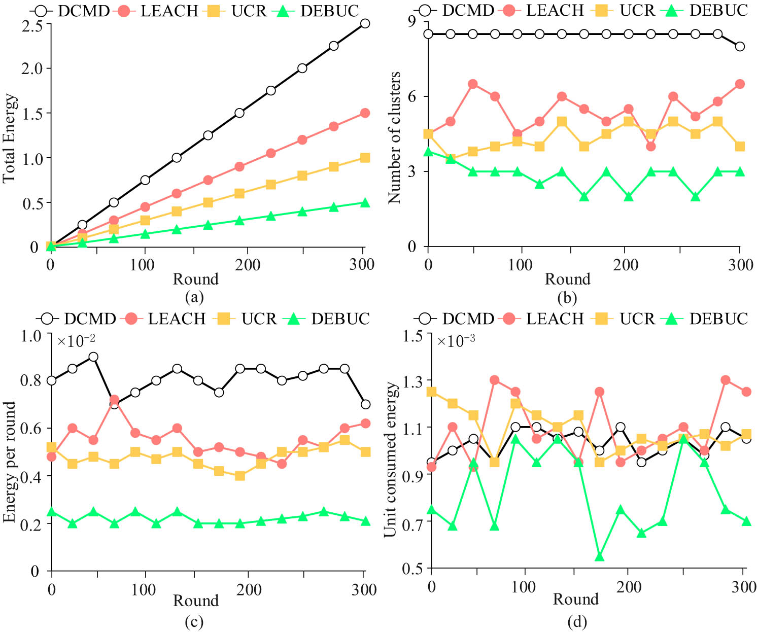
Energy efficiency comparison. (a) Energy consumption, (b) data amount, (c) energy consumption, and (d) energy efficiency.
The vertical axis in Figure 11 (a) shows that the system cumulative energy consumption can reflect the energy consumption level of a single round of data collection, that is, the average energy consumption can provide feedback on the performance of the algorithm. Among them, the system energy accumulation speed of DCMD was the fastest, while the system energy accumulation speed of DEBUC was the slowest, indicating that the algorithm performance of DCMD was the best. The vertical axis in Figure 11 (b) represents the number of clusters generated by the algorithm, which can provide feedback on the stability of data collection in each round of the algorithm. The DCMD algorithm was stable at around 8, while the other algorithms had significant fluctuations, indicating that DCMD was the most stable. The vertical axis in Figure 11 (c) shows the energy consumption level of a single round, indicating that all algorithms were relatively stable. The vertical axis in Figure 11 (d) shows the energy consumption of the smallest unit for data collection, which can provide feedback on the efficiency of the algorithm’s energy consumption. The energy consumption fluctuation value of the DCMD algorithm was about 0.2, the LEACH energy consumption fluctuation value was about 0.4, the UCR energy consumption fluctuation value was about 0.4, and the DEBUC energy consumption fluctuation value as about 0.6, indicating that the DCMD algorithm had the highest stability and energy utilization efficiency. The final comprehensive performance scores of each algorithm are shown in Figure 12.

Comprehensive evaluation score of the algorithm.
From the vertical axis in Figure 12, the comprehensive evaluation score includes three parts: life cycle, number of data packets, and monitoring quality. Among them, the DEBUC algorithm in the life cycle score had the highest score of about 13 points. The lifecycle score of the DCMD algorithm was about 8 points, the packet score was about 9 points, and the monitoring quality score was about 15 points. The highest comprehensive score of the DCMD algorithm was close to 35, indicating that the proposed dynamic clustering multi-hop data collection algorithm had strong comprehensive performance and data forwarding propagation stability.
5 Conclusion
To address the issue of data collection in WSNs, a DCMD algorithm is proposed based on clustering based data collection algorithms and mobile unit based data collection algorithms. The experiment analyzed the data collection performance, propagation stability, and sensor survival rate of the algorithm. Results indicated that DCMD only entered a significant attenuation period after 2,000 rounds, indicating that under the same conditions, the DCMD algorithm had better data transmission performance. In Scenario 1, the survival rate of the DCMD algorithm was still close to 80% at 300 rounds. In Scenario 2, the DCMD algorithm was still close to 75% at 1,500 rounds. In Scenario 3, the remaining algorithms decreased to below 50% after 100 rounds, while the DCMD algorithm remained close to 90% after 300 rounds. The remaining algorithms in Scenario 4 dropped below 50% by 500 rounds, while DCMD as still close to 70% by 1,500 rounds. From this, it can be seen that the relevant algorithms proposed in the study had significant survivability and performance advantages in various scenarios. The system energy accumulation speed of DCMD was about 50% faster on average than other algorithms, indicating that the algorithm performance of DCMD was the best. The DCMD algorithm was stable at around 8 clusters, indicating its highest stability. The energy consumption fluctuation value of the DCMD algorithm was about 0.2, the LEACH energy consumption fluctuation value was about 0.4, the UCR energy consumption fluctuation value was about 0.4, and the DEBUC energy consumption fluctuation value was about 0.6, indicating that the DCMD algorithm had the highest stability and energy utilization efficiency. The highest comprehensive score of the DCMD algorithm was close to 35, indicating its strong comprehensive performance. The research fully demonstrates that the DCMD algorithm, which integrates cluster-based data collection algorithms and mobile unit-based data collection algorithms, has significant advantages in terms of comprehensive propagation efficiency. However, the dynamic algorithm proposed in the study has a high energy consumption in large-scale scenarios and a short lifecycle under moving elements, which requires further exploration and optimization. Future research directions will focus on optimizing dynamic and clustered multi-hop data collection algorithms to reduce low energy consumption and extend the life cycle of mobile elements in large-scale scenarios. Future work will also explore new data collection algorithms, combining the advantages of cluster-based and mobile unit-based data collection algorithms to improve the integrated propagation efficiency and further improve the performance and reliability of the system.
-
Funding information: Author states no funding involved.
-
Author contribution: Weihe Zhong: study design, data collection, statistical analysis, visualization, and writing the manuscript.
-
Conflict of interest: The author declares no conflicts of interest.
-
Data availability statement: The data used to support the findings of the research are available from the corresponding author upon reasonable request.
References
[1] Z. Ballard, C. Brown, A. M. Madni, and A. Ozcan, “Machine learning and computation-enabled intelligent sensor design,” Nat. Mach. Intell., vol. 3, no. 7, pp. 556–565, 2021.10.1038/s42256-021-00360-9Search in Google Scholar
[2] M. A. Jamshed, K. Ali, Q. H. Abbasi, M. A. Imran, and M. Ur-Rehman, “Challenges, applications, and future of wireless sensors in Internet of Things: A review,” IEEE Sens. J., vol. 22, no. 6, pp. 5482–5494, 2022.10.1109/JSEN.2022.3148128Search in Google Scholar
[3] O. M. Gul, A. M. Erkmen, and B. Kantarci, “NTN-aided quality and energy-aware data collection in time-critical robotic wireless sensor networks,” IEEE Internet Things Mag., vol. 7, no. 3, pp. 114–120, 2024.10.1109/IOTM.001.2300200Search in Google Scholar
[4] P. E. Ehizuenlen, S. Apeh, and B. K. Erameh, “Context-aware energy management system for data acquisition in wireless sensor networks,” J. Res. Eng. Comput. Sci., vol. 2, no. 1, pp. 1–15, 2024.Search in Google Scholar
[5] G. Liu, “Data collection in mi-assisted wireless powered underground sensor networks: directions, recent advances, and challenges,” IEEE Commun. Mag., vol. 59, no. 4, pp. 132–138, 2021.10.1109/MCOM.001.2000921Search in Google Scholar
[6] G. M. Abdulsahib and O. I. Khalaf, “Accurate and effective data collection with minimum energy path selection in wireless sensor networks using mobile sinks,” J. Inf. Technol. Manag., vol. 13, no. 2, pp. 139–153, 2021.Search in Google Scholar
[7] S. Fu, Y. Tang, Y. Wu, N. Zhang, H. Gu, C. Chen, and M. Liu, “Energy-efficient UAV-enabled data collection via wireless charging: A reinforcement learning approach,” IEEE Internet Things J., vol. 8, no. 12, pp. 10209–10219, 2021.10.1109/JIOT.2021.3051370Search in Google Scholar
[8] Y. Wang, M. Chen, C. Pan, K. Wang, and Y. Pan, “Joint optimization of UAV trajectory and sensor uploading powers for UAV-assisted data collection in wireless sensor networks,” IEEE Internet Things J., vol. 9, no. 13, pp. 11214–11226, 2021.10.1109/JIOT.2021.3126329Search in Google Scholar
[9] T. Feng, L. Xie, J. Yao, and J. Xu, “UAV-enabled data collection for wireless sensor networks with distributed beamforming,” IEEE Trans. Wirel. Commun., vol. 21, no. 2, pp. 1347–1361, 2021.10.1109/TWC.2021.3103739Search in Google Scholar
[10] G. Li, B. He, Z. Wang, X. Cheng, and J. Chen, “Blockchain-enhanced spatiotemporal data aggregation for UAV-assisted wireless sensor networks,” IEEE Trans. Ind. Inform., vol. 18, no. 7, pp. 4520–4530, 2021.10.1109/TII.2021.3120973Search in Google Scholar
[11] L. Liu, K. Xiong, J. Cao, Y. Lu, P. Fan, and K. B. Letaief, “Average AoI minimization in UAV-assisted data collection with RF wireless power transfer: A deep reinforcement learning scheme,” IEEE Internet Things J., vol. 9, no. 7, pp. 5216–5228, 2021.10.1109/JIOT.2021.3110138Search in Google Scholar
[12] O. Mendoza-Cano, R. Aquino-Santos, J. López-de la Cruz, R. M. Edwards, A. Khouakhi, I. Pattison, et al., “ Experiments of an IoT-based wireless sensor network for flood monitoring in Colima, Mexico,” J. Hydroinf., vol. 23, no. 3, pp. 385–401, 2021.10.2166/hydro.2021.126Search in Google Scholar
[13] A. Dawson, “Robotic wireless sensor networks, big data-driven decision-making processes, and cyber-physical system-based real-time monitoring in sustainable product lifecycle management,” Econ. Manage. Financ. Mark., vol. 16, no. 2, pp. 95–105, 2021.10.22381/emfm16220216Search in Google Scholar
[14] X. Wang, M. C. Gursoy, T. Erpek, Y. E. Sagduyu, and U. A. V. “Learning-based, path planning for data collection with integrated collision avoidance,” IEEE Internet Things J., vol. 9, no. 17, pp. 16663–16676, 2022.10.1109/JIOT.2022.3153585Search in Google Scholar
[15] O. Ghdiri, W. Jaafar, S. Alfattani, J. B. Abderrazak, and H. Yanikomeroglu, “Offline and online UAV-enabled data collection in time-constrained IoT networks,” IEEE Trans. Green. Commun. Netw., vol. 5, no. 4, pp. 1918–1933, 2021.10.1109/TGCN.2021.3104801Search in Google Scholar
[16] B. Zhu, E. Bedeer, H. H. Nguyen, R. Barton, and J. Henry, “UAV trajectory planning in wireless sensor networks for energy consumption minimization by deep reinforcement learning,” IEEE Trans. Veh. Technol., vol. 70, no. 9, pp. 9540–9554, 2021.10.1109/TVT.2021.3102161Search in Google Scholar
[17] Y. Li, W. Liang, W. Xu, Z. Xu, X. Jia, Y. Xu, et al., “Data collection maximization in IoT-sensor networks via an energy-constrained UAV,” IEEE Trans. Mob. Comput., vol. 22, no. 1, pp. 159–174, 2021.10.1109/TMC.2021.3084972Search in Google Scholar
[18] X. Wei, H. Guo, X. Wang, X. Wang, and M. Qiu, “Reliable data collection techniques in underwater wireless sensor networks: A survey,” IEEE Commun. Surv. Tutor., vol. 24, no. 1, pp. 404–431, 2021.10.1109/COMST.2021.3134955Search in Google Scholar
[19] K. G. Omeke, M. S. Mollel, M. Ozturk, S. Ansari, L. Zhang, Q. H. Abbasi, et al., “DEKCS: A dynamic clustering protocol to prolong underwater sensor networks,” IEEE Sens. J., vol. 21, no. 7, pp. 9457–9464, 2021.10.1109/JSEN.2021.3054943Search in Google Scholar
[20] C. Wang, S. Zourlidou, J. Golze, and M. Sester, “Trajectory analysis at intersections for traffic rule identification,” Geo-spatial Inf. Sci., vol. 24, no. 1, pp. 75–84, 2021.10.1080/10095020.2020.1843374Search in Google Scholar
[21] A. M. Zaki, A. A. Abdelhamid, A. Ibrahim, M. M. Eid, and E. S. M. El-Kenawy, “Enhancing K-nearest neighbors algorithm in wireless sensor networks through stochastic fractal search and particle swarm optimization,” J. Cybersecur. Inf. Manag. (JCIM), vol. 13, no. 1, pp. 76–84, 2024.10.54216/JCIM.130108Search in Google Scholar
[22] Y. Singh and T. Walingo, “Smart water quality monitoring with IoT wireless sensor networks,” Sensors, vol. 24, no. 9, pp. 2871–2822, 2024.10.3390/s24092871Search in Google Scholar PubMed PubMed Central
[23] K. K. Kumar and G. Sreenivasulu, “An efficient routing algorithm for implementing internet-of-things-based wireless sensor networks using dingo optimizer,” Eng. Proc., vol. 59, no. 1, pp. 212–219, 2024.10.3390/engproc2023059212Search in Google Scholar
© 2025 the author(s), published by De Gruyter
This work is licensed under the Creative Commons Attribution 4.0 International License.
Articles in the same Issue
- Review Article
- Enhancing IoT network security: a literature review of intrusion detection systems and their adaptability to emerging threats
- Research Articles
- Intelligent data collection algorithm research for WSNs
- A novel behavioral health care dataset creation from multiple drug review datasets and drugs prescription using EDA
- Speech emotion recognition using long-term average spectrum
- PLASMA-Privacy-Preserved Lightweight and Secure Multi-level Authentication scheme for IoMT-based smart healthcare
- Basketball action recognition by fusing video recognition techniques with an SSD target detection algorithm
- Evaluating impact of different factors on electric vehicle charging demand
- An in-depth exploration of supervised and semi-supervised learning on face recognition
- The reform of the teaching mode of aesthetic education for university students based on digital media technology
- QCI-WSC: Estimation and prediction of QoS confidence interval for web service composition based on Bootstrap
- Line segment using displacement prior
- 3D reconstruction study of motion blur non-coded targets based on the iterative relaxation method
- Overcoming the cold-start challenge in recommender systems: A novel two-stage framework
- Optimization of multi-objective recognition based on video tracking technology
- An ADMM-based heuristic algorithm for optimization problems over nonconvex second-order cone
- A multiscale and dual-loss network for pulmonary nodule classification
- Artificial intelligence enabled microgrid power generation prediction
- Special Issue on AI based Techniques in Wireless Sensor Networks
- Blended teaching design of UMU interactive learning platform for cultivating students’ cultural literacy
- Special Issue on Informatics 2024
- Analysis of different IDS-based machine learning models for secure data transmission in IoT networks
- Using artificial intelligence tools for level of service classifications within the smart city concept
- Applying metaheuristic methods for staffing in railway depots
- Interacting with vector databases by means of domain-specific language
- Data analysis for efficient dynamic IoT task scheduling in a simulated edge cloud environment
- Analysis of the resilience of open source smart home platforms to DDoS attacks
- Comparison of various in-order iterator implementations in C++