Analysis of different IDS-based machine learning models for secure data transmission in IoT networks
-
Dejana Gladić
 ,
Jelena Petrovački
,
Srdan Sladojević
,
Jelena Petrovački
,
Srdan Sladojević

Abstract
The Internet of Things (IoT) encompasses a network of interconnected devices that collect, analyze, and exchange vast amounts of data. However, this connectivity creates opportunities for various types of cyberattacks, making IoT systems vulnerable and potentially leading to the compromise of sensitive information. Therefore, developing effective intrusion detection system (IDS) is one of the key challenges in IoT network security. The aim of this study is to develop a machine learning (ML) model for network traffic classification and attack detection in IoT environments. Through a comparative analysis of different algorithms, the study seeks to identify the model with the best performance, which could serve as a foundation for efficient IDS solutions tailored to the specific characteristics of IoT networks. The RT-IoT2022 dataset was used for experimental analysis, providing realistic framework for testing ML models, including k-nearest neighbors, Random Forest, XGBoost, multilayer perceptron, and various 1D convolutional neural network architectures. The study examines preprocessing techniques, focusing on dimensionality reduction (principal component analysis, variance inflation factor, Pearson’s test), outlier detection (interquartile range, Z-score, Isolation Forest), and transformation methods (Box–Cox, RobustScaler, Winsorization). Based on the results of the experiment, the most effective model and preprocessing technique were proposed.
1 Introduction
With the development of Internet technologies, the volume of generated data has increased. A significant portion of generated data come from Industry 4.0, where Internet of Things (IoT) is a key component. On the perception layer of IoT (presented in Figure 1), devices and sensors collect data from the environment and forward it to the network layer, which enables data transmission to other devices and applications on the application layer [1]. Industrial IoT (IIoT) devices and other smart resources are sources of data that provide insight into the functioning of an industrial system. Collecting and processing these heterogeneous data, it is possible to improve system monitoring. Using advanced analytics techniques, organizations can harness the full potential of Industry 4.0 data to achieve competitive advantage and growth. When implementing Industry 4.0 big data analytics platforms, it is very important to identify potential security risks specific to industrial systems to ensure the integrity of the data infrastructure. Without adequate protection, the industrial system can face unauthorized access, leading to data misuse and issues in the company’s sustainability.
![Figure 1
(A)NIDS architecture (adapted from the study of Karanam [9]).](/document/doi/10.1515/comp-2025-0032/asset/graphic/j_comp-2025-0032_fig_001.jpg)
(A)NIDS architecture (adapted from the study of Karanam [9]).
Each layer of an (I)IoT architecture is vulnerable to malicious attacks. This article focuses on attacks targeting the network layer that is susceptible to vulnerabilities due to insecure communication protocols, various device connection standards, and weak authentication mechanisms. Examples include attacks on connections using Secure Shell (SSH) or Hypertext Transfer Protocol (HTTP) protocols [2].
One solution to prevent hacker attacks on the network is implementing an intrusion detection system (IDS), an software whose role is to observe a system and detect harmful behavior. IoT networks typically consist of a large number of interconnected devices with limited physical resources, which complicates the implementation of this software within each device. For this reason, the focus of this research is on analyzing network-based IDSs (NIDSs). NIDS is a specific type of IDS designed to observe traffic through the entire network to detect harmful behavior [3].
This study emphasizes anomaly-based NIDS (ANIDS), a type of NIDS, that monitors user behavior over time to establish a model of normal activity. If some activity occurs, which is suspicious and deviates from the expected behavior, it is marked as harmful, i.e., as an anomaly [4]. By detecting an anomaly, an alarm could be activated (Figure 1) that would emphasize that there is a problem and that it is necessary to respond adequately in time and prevent possible damages. ANIDS is only as successful as it is effective in deciding whether to identify an activity as a malicious attack. ANIDS is very effective in detecting new attacks, but it has a disadvantage of a high rate of false alarms, i.e., lower accuracy [5]. Additionally, detecting an attack does not reveal the reason why it occurred [1].
There are different ways to implement ANIDS: (i) statistical models (statistical-based approach), (ii) protocol verification (knowledge-based approach), (iii) rule-based approach, and (iv) machine learning (ML)-based approach [1]. Each of these approaches has drawbacks: protocol verification can produce false positives (FP) when faced with unknown protocols, and rule-based methods fail to detect new, unknown attacks [6]. To minimize the previously mentioned drawbacks of ANIDS, it is essential to choose an appropriate implementation approach.
This research adopts the ML-based approach because the process of identifying attacks in the IoT environment can be improved by applying specific ML algorithms, trained and tested on data exclusively from IoT networks. This type of ANIDS has the ability to learn patterns of network traffic to detect attacks more easily later, even those that are not previously known. This approach can achieve high accuracy in attack detection and reduce false alarms, but the downside is that training the model requires a large amount of memory and processing resources [7]. Additionally, attack patterns frequently change to make detection more difficult, so it is necessary to periodically retrain the models on newer datasets [8]. The aim of this study is to conduct a comparative analysis of various supervised and deep learning models to determine the optimal ML model for implementing an ANIDS based on their performance. The task of the models is to perform binary classification, categorizing network traffic into normal traffic (without attacks) and traffic that has been affected by an attack.
To adequately detect attacks and to ensure precise and meaningful insights, flow-based analysis can be performed. Here, we give preference to flow-based, which analyzes the entire traffic and continuously monitors changes, rather than packet-based analysis. Flow-based analysis enables real-time anomaly detection, which is essential for timely attack responses. Flow is bidirectional, in our case, which enables continuous interaction between devices, and this is crucial for efficient management and automatic adjustment of systems in the IoT environment.
The development of ML models for attack detection is based on data collected from real-time IoT infrastructure. These data are tabularly organized and originate from the publicly available RT-IoT2022[1] dataset, whose granularity corresponds to the previously selected type of analysis, flow-based analysis.
(I)IoT network infrastructure has its own specificities in relation to the general network infrastructure. The ANIDS implemented in an IoT environment must efficiently process, analyze, and respond to data packets across various network layers, within a heterogeneous network [9]. Many IoT devices use specialized packet transfer protocols such as Message Queuing Telemetry Transport (MQTT) and Constrained Application Protocol (CoAP). The IoT network generates large amounts of diverse data so ANIDS implemented for IoT should process high volume of data in a short time and generate a response quickly [6]. Furthermore, there are specific behavioral patterns within IoT environments, such as Distributed Denial of Service (DDoS) attacks. Existing ANIDS implementation does not sufficiently address the specificities of IoT infrastructure, resulting in degrading ANIDS performance and weaker attack detection. This specific characteristic of IoT network infrastructure further reinforces the previously made conclusions regarding the implementation approach of the ANIDS system.
The generalized conceptual architecture of an NIDS system is shown in Figure 1. The focus of this article is on the part of the application layer that relates to developing ML models and selecting appropriate techniques for data preprocessing.
To summarize, the goal of this research is to develop an ML-based ANIDS designed for detecting cyber attacks in IoT network. In this regard, goal is to train ML algorithms that perform the binary classification process, classifying network traffic as normal or attack-related. For the development of the models, a publicly available dataset RT-IoT2022 is used, which describes normal and problematic communication within the network of connected IoT devices. Although the data used for training the models do not strictly originate from the industrial domain, the communication patterns observed in IoT networks can be leveraged for identifying patterns in IIoT networks as well. ML enables learning transfer, meaning that models trained on IoT traffic can serve as a foundation for adapting intrusion detection in IIoT systems.
We have developed the following models: logistic regression (LR), Random Forest (RF), k-nearest neighbors (KNN), Extreme Gradient Boosting (XGBoost), multilayer perceptron (MLP), and one-dimensional convolutional neural network (1D CNN).
Given that traditional ML models such as KNN, RF, XGBoost, and MLP have a simpler architecture compared to CNN, we evaluated their performance in the first research phase to identify the best-performing model for our task. After analyzing the results, we recognized opportunities to enhance preprocessing techniques to improve model performance. Additionally, we found that more complex models are better equipped to capture complex patterns within the large volume of data available in the selected dataset. In the second phase, we enhanced the preprocessing techniques and selected the 1D CNN for further evaluation. Due to the complexity of the 1D CNN, six different architectures were developed to identify the one that best fits the data. The best-fit 1D CNN model was then compared against the best-performing model from the first phase on the research to determine whether the more complex architecture and improved preprocessing methods provided a notable improvement in performance. We evaluated and compared the results of proposed models using various metrics described in this article. Our assumption that the CNN would deliver better results proved to be correct, leading us to select the 1D CNN architecture with the highest performance as the most effective model. The developed and tested ML model is now ready for integration into an ANIDS, which can be implemented at the network layer of industrial systems. By leveraging this advanced model, the ANIDS can significantly enhance its threat detection capabilities, providing a robust defense against cyber attacks in industrial environments.
This article presents an extended version of Gladic et al. [10], which is different from the previously published article in the following aspects:
We expanded the literature review to include findings from studies that develop more complex ML model architectures. Theoretical foundations of all developed models are thoroughly explained. Additionally, it has been systematically structured into distinct sections covering theoretical foundations of the models, their practical applications in previous research, and an overview of available datasets along with their usage in conducted studies.
Additional data preprocessing techniques have been applied to the selected dataset, specifically for detecting and reducing outliers. Isolation Forest (IF) was used for outlier detection, while Winsorization and RobustScaler were applied for outlier reduction. These techniques resulted in new versions of the original dataset, which have been visualized in this study:
A detailed description and analysis of six different 1D CNN model architectures are provided, along with their experimental results. The models described in the study by Gladic et al. [10] have been retained in this version as well.
The discussion on model performance has been expanded to include an analysis of the results obtained from the developed 1D CNN models.
The explainability of the predictions of the selected ML model has been verified using the shapley additive explanations (SHAP) method.
2 Related work
One of the key steps in developing an ML-based ANIDS is selecting an ML model that will adequately classify attacks and distinguish them from normal activities. In this section, we will provide a comprehensive overview of ML models used in this domain, their applications in other studies, and commonly analyzed datasets containing IoT network data used to enhance security. Additionally, we will explore the models utilized with these datasets and review the existing literature on the dataset chosen for our research.
2.1 Overview of ML models and their application
To properly develop and train supervised models, it is important to understand their fundamental characteristics. In this section, we describe the following ML models: KNN, LR, support vector machine (SVM), decision tree (DT), RF, XGBoost, MLP, and CNN. The models are chosen for their key advantages, while their potential weaknesses can be further analyzed depending on the specific usage, some of which are examined in this research.
KNN is a method for classification and regression that assigns a new instance to the most common class among its KNNs. It usually uses Euclidean distance to measure similarity between instances [11–14]. LR is a method for binary classification that models the relationship between a dependent variable and one or more independent variables. It predicts the probability of class membership and applies a threshold to assign a class label [15]. SVM finds the best hyperplane that separates classes by maximizing the margin between support vectors. For non-linear data, kernel functions transform it to a higher dimension for better separation [12,16]. DT uses a tree structure where internal nodes test attribute values, branches show outcomes, and leaves give the final prediction [17]. RF improves classification by combining multiple DTs, each trained on random samples and features, which helps reduce overfitting and increases stability. It calculates feature importance and classifies new instances through majority voting [12,18]. XGBoost is an ensemble model that improves classification by combining multiple simple models. It uses gradient boosting, where each model learns from the mistakes of the previous one, leading to better accuracy [12,19]. MLP is a fully connected neural network (NN) used for classification and regression. It has three layers: input, hidden, and output, with neurons connected across layers. These connections help the network learn complex patterns and generate outputs [20–22]. CNNs are a type of NN used for analyzing images, videos, and sequential data. They apply filters in convolutional layers to detect patterns, use ReLU for activation, and reduce dimensionality with pooling layers. Finally, fully connected layers classify samples, such as detecting attacks. CNN models are more efficient than MLP [1,21,23–25].
In Table 1, we summarize the applications of different ML models, that are presented in various studies, alongside with noticed advantages and potential weaknesses of analyzed models. Based on these results, we have decided to focus on KNN, RF, XGBoost, MLP, and CNN. In contrast, DT and SVM were not considered suitable for our purposes. SVM was not chosen because it is not well suited for large datasets and imbalanced data, while DT tends to overfit. LR has been selected as the baseline model (BLM).
ML model review
| Ref. | Models | Advantages | Disadvantages |
|---|---|---|---|
| [11–14] | KNN | – Simple and adaptable | – Selecting parameter values can significantly impact performance |
| – More resistant to noise | – Can be slow during execution | ||
| [15] | LR | – Simple and interpretable method | – Assumes a linear relationship |
| – Can be sensitive to outliers | |||
| – Threshold needs to be carefully selected | |||
| [12,16] | SVM | – Generalizes well | – Choice of kernel and hyperparameters affects adaptability |
| – Not flexible for large/unbalanced datasets | |||
| – Poor at detecting DDoS | |||
| [17] | DT | – Easy to interpret and visualize | – Tendency to overfit |
| – Sensitive to data changes | |||
| [12,18] | RF | – Automatically handles missing data | – Higher memory and processing requirements |
| – Robust with unbalanced data | |||
| – High accuracy in attack detection | |||
| [12,19] | XGBoost | – Speed and efficiency from parallelization | – Higher computational cost |
| – Robust with unbalanced data | – Performance depends on hyperparameters | ||
| – Extensive optimizations | |||
| [20–22] | MLP | – Recognizes complex patterns and non-linearities | – Requires more training time |
| – Large number of parameters | |||
| – No dimensionality reduction | |||
| [1,21,23–25] | CNN | – Convolutional layers select relevant features | – Can be computationally expensive on large datasets |
| – Faster learning than MLP and uses less memory | – Requires considerable training time | ||
| – No need for intensive preprocessing |
2.2 Overview of datasets in IoT environments and models applied to these datasets
The model’s performance depends not only on its architecture but also on the quality and size of the dataset on which it was trained. A review of the literature revealed that several commonly used datasets represent network traffic in IoT environments, with the most common being KDDCup99[2], NSL-KDD[3], UNSWNB15[4], CICIDS2018[5], and RT-IoT2022. Their advantages and disadvantages are described in the study by Sharmila and Nagapadma [26] and Moustafa and Slay [5]. For each, as well as some additional ones in the field of IDS, models that were trained and evaluated using them will be presented to gain insight into the state of the field and identify ideas that we can apply in our research, considering that we are dealing with the same topic.
In article by Balakrishnan et al. [27], an analysis of the KDDCup99 dataset was performed, which aimed to detect attacks, and a new feature selection algorithm called optimal feature selection (OPT) was proposed. Of the ML models, rule-based classifier (RBC) and SVM were used. The study by Balakrishnan et al. [27] is focused on the way in which the proposed feature selection algorithm reduces the time that would otherwise be required for error detection. Considering the importance of optimizing attribute selection for attack detection, we will also pay attention to similar methods in our research.
KDDCup99 dataset is widely used for intrusion detection research, some of them mentioned in this section; it has several significant drawbacks, such as a large number of duplicate and redundant records, leading to model bias towards the most common attack patterns. Additionally, the uneven data distribution causes certain classes, such as DoS attacks, to dominate, while others, such as User to Root (U2R) attacks, are significantly rarer, complicating accurate classification. Furthermore, the dataset does not fully reflect real network conditions and the variability of contemporary network traffic. To address these issues, the NSL-KDD dataset was created as an improved version of KDDCup99, which removes duplicates, balances the data distribution, and provides a more realistic environment for evaluating intrusion detection models [28].
Lihua [29] used MATLAB to analyze the NSL-KDD dataset. The goal of the research was to create a ML model that will be used in energy-aware IDS (EIDS) to ensure safe and reliable data transmission between vehicles in Internet of Vehicle environments with optimal energy consumption. The algorithms used are regression algorithms, SVM, RF, MLP, and DT algorithms. Regression algorithms performed best, from the point of view of accuracy, followed by the RF algorithm. In our research, we are using the RF algorithm because of the advantages it has shown in the study by Lihua [29].
The dataset UNSW-NB15 is analyzed in previously published articles [30,31]. In the study by Hammad et al. [30], Feature Reduction (FR) is used for attribute selection as well as attribute ranking using the Correlation-based Feature Selection (CFS) technique, while J48, RF, ZeroR (supervised learning), and K-Means (unsupervised learning) algorithms are used for anomaly detection. The measurement criteria were, among other things, the accuracy and precision of the algorithm. The RF algorithm performed best, followed by J48. The UNSW NB15 dataset contains about 2.5 million records. Therefore, in the study by Faker and Dogdu [31], deep NN (DNN) techniques, but also RF and Gradient Boosting Tree (GBT) are used on this dataset. Homogeneity metric is used for feature selection, while fivefold cross-validation (CV) is used for performance analysis. The Apache Spark[6] is used alongside its ML library as well as the Keras deep learning library[7]. And these articles give preference to RF, as well as deep learning techniques.
In the study by Ali et al. [20], MLP was tested on the KDDCup99 and UNSWNB15 datasets. To optimize the learning process and reduce the error rate in attack detection, the gray wolf optimization (GWO) algorithm was used to tune parameters such as weights and biases. The proposed hybrid GWO–MLP IDS demonstrates high efficiency in detecting cyber-attacks by optimizing NN parameters. Ali et al. [20] confirm that hyperparameter optimization can play a key role in improving the performance of MLP models in attack detection, which can be useful for our future research in this field.
In the article by Berbiche and Alami [32], the CICIDS2018 DDoS attacks dataset was examined, where experiments were conducted using various feature selection techniques and over-sampling methods for data balancing, including adaptive synthetic sampling approach (ADASYN), synthetic minority oversampling technique (SMOTE), and its variation Borderline-SMOTE. Subsequently, different models were evaluated, with MLP chosen for testing due to its ability to identify complex patterns in the data. However, MLP has shown to require longer training times and exhibits instability when classifying synthetic data, so caution is necessary when selecting the data balancing method. The focus of the study by Ali et al. [33] is the development of CNN-based models in real-world NIDS. The system design consists of offline training and online attack detection without intensive data preprocessing. A specific feature of this work is that after the last convolutional layer, no pooling layer is applied; instead, a fully connected layer is used. The model was trained on the raw and feature CICIDS2018 dataset, achieving over 99% accuracy and outperforming SVM as well as the deep belief network. Berbiche and Alami [32] confirm the importance of data balancing using the SMOTE technique and its variants, which is relevant to our research, given that we have also applied SMOTE, as well as both models that have shown good results in both mentioned studies (MLP and CNN).
The performance of the CNN model, in comparison with recurrent NN (RNN), was also examined in the study by Kim et al. [23], where the model was trained on the KDDCup99 and CICIDS2018 datasets. The authors first converted the data into grayscale and RGB image datasets, which were then used as input for the algorithm. Experiments were conducted by varying parameters such as kernel size and the number of convolutional layers, and both binary and multiclass classification were evaluated. The CNN model achieved 99% accuracy on the KDDCup99 dataset and 91.5% accuracy on the CICIDS2018 dataset. Experiments conducted on CNN architectures with different kernel sizes and network depths were also evaluated in our research paper.
Jovanović and Vuletić [34] explain the potential problems associated with using publicly available datasets. They resort to creating a new dataset that they will use to train their model, based on the publicly available IoT-23[8] dataset that they will use for verification. Their research is based on intra-flow analysis of traffic, which involves analyzing characteristics such as the number of forwarded packets or the number of bytes within a single flow. Another approach to the research would be to analyze the content of each packet, which is an approach that requires a much larger amount of resources. For traffic classification, KNN, LR, and RF were used, and binary classification was performed, allowing conclusions to be drawn about the presence of an attack but not about the specific type of attack. To optimize the model development process and save resources in terms of memory and power consumption, dimensionality reduction was performed by calculating and analyzing the receiver-operating characteristic (ROC) and area under the curve (AUC) values for each feature. Additionally, a heatmap was used to analyze the correlation between different features. Through their analysis, the authors conclude that KNN and LR produced quite good and similar metric results. Considering that LR consumes less memory, which plays a significant role for systems like IDS, this model was given preference [34]. In this article, we used heat maps as one of the methods for analyzing correlation and attribute selection, along with the application of KNN, RF, and LR as BLM.
In the study by Ullah and Mahmoud [24], 1D CNN is mentioned, for which it is not necessary to convert inputs into images; it is sufficient to transform the input into a two-dimensional format, which is most commonly used for time-series or sequential data. In addition, 1D CNN, 2D CNN, and 3D CNN were evaluated on an integrated set of various datasets (BoT-IoT, MQTT-IoT-IDS2020, IoT-23, and IoT-DS-2 datasets). The F1-score of the 1D CNN model is 99.95%. There are not many articles that focus on 1D CNNs. However, due to the specific characteristics of the dataset chosen for our research, it is essential to utilize this type of CNN.
The analysis of datasets and the performance of the models applied to them confirmed the decision to focus on KNN, RF, XGBoost, MLP, and CNN models in this research.
2.3 RT-IoT2022 dataset – description and use cases
For the purposes of this study, the dataset RT-IoT2022 is used. The RT-IoT2022 dataset consists of recent, real-world data collected from IoT devices such as ThingSpeak-LED, Wipro-Bulb, and MQTT-Temp, and Amazon Alexa as well as simulated attack scenarios. The dataset contains data on a variety of attack types, including not only DDoS and SSH attacks, which are commonly found in other datasets, but also scan and Man in the Middle (MITM) types of attacks. This diversity can influence the development of models that will be optimized for classifying specific types of attacks, thereby increasing the efficiency and accuracy of detection. Additionally, the number of instances is sufficiently large for training some more complex ML models while not requiring excessive computational resources for conducting experiments. To gain a comprehensive insight into existing ML solutions applied to the selected dataset, it is necessary to conduct a detailed analysis of relevant approaches, which will allow for the identification of potential improvements and contribute to the further development of this field.
Sharmila and Nagapadma [26] construct and train an auto-encoder as an unsupervised learning technique on normal network traffic behaviors with the aim of detecting anomalies. In this article, compared to the study by Sharmila and Nagapadma [26], supervised learning techniques are used, specifically classification techniques. Prasad et al. [35] present a hybrid model TTOS-RAAM that uses min–max scaling for data normalization and a technique called Coati–gray wolf optimization (CGWO) for selecting the most important features. Attacks are detected using a method called conditional variational autoencoder (CVAE), and its parameters are adjusted using improved Chaos African vulture optimization. The research was conducted on the RT-IoT2022 dataset, with TTOS-RAAM achieving an accuracy of 99.91%. Unlike Prasad et al. [35], in this article, we scaled the data by applying standard deviation and mean.
Almohaimeed and Albalwy [36] tested the MLP model on the clean RT-IoT2022 dataset, as well as on the dataset obtained by applying various feature selection techniques, including information gain, gain ratio, CFS, Pearson’s correlation, and symmetric uncertainty. They also analyzed the correlation between certain features and their impact on attack detection. The lowest F1-score was achieved by evaluating the MLP model on the clean dataset, while the highest was on the dataset where all mentioned feature selection techniques were applied. During this research, we evaluated the model results on both the cleaned and raw dataset.
The detection of attack types in the study by Arabiat and Altayeb [37] is achieved by training models such as RF, artificial NN (ANN) (type not specified), LR, and SVM. The authors applied linear discriminate analysis, which reduced the number of records in the dataset. Experimental results show that RF achieved a classification accuracy of 99.9%, while ANN had 99.8%. RF and MLP, a type of ANN, are also candidates for training and evaluation in this article, but with the application of different preprocessing techniques.
Elzaghmouri et al. [38] present a hybrid deep learning architecture that combines CNN, bidirectional LSTM, gated recurrent units (GRU), and attention mechanisms for effective threat detection in IoT. The model was evaluated on the RT-IoT2022 dataset and showed exceptional accuracy and precision, surpassing traditional algorithms and significantly improving the security of IoT networks. The proposed model achieved an F1-score of 99.61 and a false-positive rate (FPR) of only 0.00084. One of the future ideas is to train the model using attention mechanisms, as this approach allows models to focus on relevant parts of the input data.
Another article addressing the selected dataset is Ahmed et al. [19]. In this research, a detailed feature analysis was conducted using box plots and heat correlation maps to adequately clean the data and perform the selection of necessary attributes. On the processed data, min–max standardization and SMOTE balancing were applied. Traditional models such as CatBoost, Extra Trees, RF, XGBoost, and LightGBM were tested, and the models were trained using 10-fold CV. The best performances were shown by XGBoost and LightGBM, with achieved accuracies of 99.55 and 99.65%, respectively. All mentioned articles perform multi-class classification according to the type of attack on the selected dataset, while in this article, binary classification is performed to indicate whether an attack occurred or not. Box plots, heat maps for exploratory data analysis, SMOTE as a balancing technique, and RF and XGBoost models were also analyzed in our study.
2.4 Summary overview: characteristics of the dataset and conducted research on them
Since there is a conclusion that there is no universal architecture for ML models applicable to all IoT data datasets, the following characteristics of the processed datasets are highlighted to provide the scientific community with a starting point for directing their research on their data corpus. Different architectures are designed based on the use case, the recorded characteristics of network traffic, and the size of the traffic sample [39]. Therefore, these characteristics could serve as a starting reference for the future direction of research. In addition to the mentioned characteristics of the datasets, Table 2 includes references to the papers, processed models, attribute selection techniques, and the model selected as the most suitable. In Table 2, data of the most frequently used publicly available datasets are presented, as well as models applied on them.
Summary of literature review
| Ref. | Dataset | Record number | Feature number | Attack types | Selected ML models | Attribute selection methods | The best ML model |
|---|---|---|---|---|---|---|---|
| [27] | KNN | 5209460 | 41 | DoS, Probe, R2L, U2R | RBC, SVM | OPT | OPT-focused SVM |
| [23] | CNN, RNN | Not applied | CNN | ||||
| [29] | NSLKDD | 148517 | 41 | DoS, Probe, R2L, U2R | Regression ML models, SVM RF MLP, DT | Not applied | RF, regression ML models |
| [30] | UNSW-NB15 | 2540044 | 49 | Fuzzers, Analysis, Backdoors, DoS, Exploits, Generic, Reconnaissance, Shellcode, Worms | J48, RF, ZeroR, K-Means | FR, CFS | RF, J48 |
| [31] | DNN, RF, GBT | Homogeneity metric | DNN | ||||
| [23] | CICIDS2018 |
|
80 | Brute-force, Heartbleed, Botnet, DoS, DDoS, Web attacks, Internal infiltration | CNN, RNN | Not applied | CNN |
| [33] | CNN, SVM | Not applied | CNN | ||||
| [26] | RT-IoT2022 | 123117 | 85 | ARP poisoning, DDOS Slowloris, DOS SYN Hping, Metasploit Brute Force SSH, NMAP scans | Quantized Autoencoder (QAE) | Not applied | QAE |
| [35] | Conditional Variational Autoencoder (CVAE) | Coot-gray wolf optimization (CGWO) | CVAE | ||||
| [36] | MLP | Information gain, gain ratio, correlation-based selection, Pearson’s correlation, symmetric uncertainty | MLP | ||||
| [37] | RF, ANN, LR, SVM | Not applied | RF | ||||
| [38] | CNN, bidirectional LSTM, GRU, attention mechanisms | Not applied | CNN, bidirectional LSTM, GRU, attention mechanisms | ||||
| [19] | CatBoost, Extra Trees, RF, XGBoost, LightGBM | Heat-maps | XGBoost, LightGBM |
3 Methodology
In this section, we present a detailed overview of the dataset, covering its characteristics, the preprocessing steps, and the model development process.
3.1 Dataset and preprocessing
The dataset RT-IoT2022 was chosen for the development and testing of the ML model. It is mentioned in Section 2.2, and it is compared with datasets of a similar type and purpose. The dataset was created based on the actual behavior of the IoT network infrastructure. The process of dataset creation, including its methodology and underlying principles, is thoroughly described in the study by Sharmila and Nagapadma [26]. The attribute values were recorded using the Zeek network monitoring tool and the Flowmeter plugin. The collected Packet Capture (PCAP) files were then converted and exported as Comma-Separated Value files using the CICFlowmeter tool, which generates bidirectional flow-based time-related features that help distinguish attacks [26]. IoT devices within this dataset are classified as victim devices and attacker devices. Distinguishing between them can be challenging, as attacker devices often change their IP addresses to avoid detection. Although the data do not have an explicit time-related attribute, it is organized sequentially, which plays a significant role in the selection and understanding of the ML model. The data are aggregated at the bidirectional flow level. Each instance corresponds to a single established communication.
The downloaded version of the dataset was created in April 2024 and contains 123,117 instances and 85 features. Among the attributes of this dataset, the target variable related to the type of attack was carefully selected, because it best fits the goal of this research – the development of a model that will predict whether an attack has occurred or not. There are no missing values among the data. The initial dataset structure includes 82 numerical and 3 categorical variables. Categorical variables, including the target variable, were converted to numerical ones so that they could be used in the development of ML models. The variable used to generate the target variable, attack_type, indicates whether an attack occurred in the process of communication between two devices, as well as the type of the attack. The dataset contains various types of attacks, which can be classified into four groups based on their specific characteristics: (i) DDoS, (ii) scan attack, (iii) MITM, and (iv) SSH brute-force. DDoS attacks are multi-connection attacks where the attacker sends a large number of unnecessary packets through the network, exhausting server resources and slowing down the network [6]. Scan attacks are multi-connection attacks aimed at scanning the network to identify open ports and vulnerable services, allowing the attacker to find potential targets for further attacks. SSH brute-force attacks are single-connection attacks that attempt unauthorized access to another device by trying different combinations of usernames and passwords, aiming to take control of the device and execute commands [26]. MITM attacks are single-connection attacks that redirect network traffic to the attacker’s device, enabling eavesdropping and data manipulation. In order to predict whether an attack has occurred or not the attack_type variable is transformed so that the new target variable includes the values 0 and 1, where instances representing normal network behavior are mapped to the value 0, while instances with any attack type are mapped to the value 1. In Table 3, the classes of the target variable are presented, including the newly encoded values of the target variable, the meaning of each value, the number of instances corresponding to each class, and their contribution relative to the total number of dataset instances. An uneven distribution among the classes can be observed. Later in this article, applied techniques for balancing the data will be described.
Distribution of target variable classes
| Encoded_attack value | Encoded value meaning | Number of instances | Percentage of instances (%) |
|---|---|---|---|
| 1 | Attack occurred | 110610 | 89.84137 |
| 0 | Normal behavior | 12507 | 10.15863 |
The next step is the verification of the initial set of hypotheses, in order to verify the correctness of the data. The hypotheses are as follows:
H1 – Flags are set only in communication conducted via the Transmission Control Protocol (TCP).
H2 – Network congestion is a good opportunity for a hacker to attack the network.
Flags are sent in packet headers to signal different phases and states of the connection between two devices. Each tuple in the dataset has a value indicating the type of protocol used (TCP, Internet Control Message Protocol [ICMP], User Datagram Protocol [UDP]) as well as the number of flags sent. Packets with flags are transmitted only via the TCP/IP protocol, but not with UDP and ICMP. The number of sent flags for the tuples related to ICMP or UDP protocols must not be greater than zero. Otherwise, the tuples are considered invalid. However, for TCP, having more than zero flags is acceptable. The result of this analysis is that the data are correct, confirming hypothesis H1. The explicit congestion notification flag set by the receiver, as well as the response to it in the form of the congestion window reduced (CWR) flag, signals that there is network congestion in communication. The response to the presence of the CWR flag would be to reduce the send window size. Analyzing the data, we conclude that the CWR flag was sent 23 times, but that the window size was not reduced even once. Furthermore, the correlation of the target variable and the cases in which network congestion occurred is checked. Pearson’s correlation test calculated a coefficient of
After verifying data accuracy, we reduced dimensionality and processed outliers. We first applied dimensionality reduction techniques and then trained various models on the resulting datasets. As we tested a wider range of models, we identified the need to adjust the input dataset to fit the specific characteristics of each model. To address this, we explored different combinations of feature selection and outlier processing. The following paragraphs and the accompanying Figure 2 present the combinations that produced the most relevant results for further model training.

Scenarios and datasets: overview.
As mentioned Section 1, the development of models and the evaluation of their performance were conducted in two phases. Traditional ML models (KNN, RF, XGBoost, and MLP) are evaluated in the first research phase. In the second phase, we improved upon the first by developing new ML models that could potentially achieve better results.
In the feature selection process, a combination of the following techniques was used: variance analysis using principal component analysis (PCA), variance inflation factor (VIF), and checking correlations via heat map using Pearson’s test. Although these techniques identified key features, the results were not completely consistent, making it difficult to select adequate features. To overcome this challenge, the union of these results was used as a basis for feature selection, with additional consideration of the importance of each feature in the context of the real system under study. In the first research phase, the resulting dataset (RTIoT2022-v1, on the left-hand side of Figure 2) consists of 52 features, reduced from the initial 85. In the second phase, the dataset is revised once more, resulting in a redacted dataset with 48 features.
Visual techniques such as histograms and boxplots were used to analyze data distribution and identify potential outliers. In the first phase of research, we decided to train the models regardless of the presence of outliers. Although the presence of outliers was observed in a smaller percentage, it was decided to keep them because the features where these outliers were observed are identified as potential indicators of hacker attacks.
In the second phase of the research, which followed the completion of the first phase, we tested various techniques for outlier detection and subsequently applied outlier reduction methods. In this article, we present two scenarios in the second phase of our research. The scenarios are enumerated as Sc. 1 and Sc. 2 on the right-hand side of Figure 2. The second scenario further includes two sub-scenarios, labeled as Sc. 2.1 and Sc. 2.2 on Figure 2.
In the first scenario (Sc. 1), we used the IF algorithm for outlier detection. This method is based on the principle of randomly segmenting the data using hierarchical trees. Unlike statistical methods that measure the distance of points from the mean, IF actively isolates outliers since they are typically easier to separate from the rest of the data.
Outliers were most prevalent in the feature flow_duration, which contains data of the duration of an established network flow. Figure 3 presents a boxplot for the flow_duration feature values, illustrating the data distribution and potential outliers. Most of the data are concentrated in a narrow range near zero, indicating a high density of smaller flow_duration values. However, we observe a large number of outliers with significantly higher values, suggesting a long-tailed (right-skewed) distribution. These outliers may represent extremely long sessions or unusual network activity. Also, the calculated skewness value of 120.96 indicates an extremely right-skewed distribution. Ideally, skewness value should be as close to zero as possible.

Boxplot for flow_duration.
We applied three techniques to transform critical values and analyzed their results. Log transformation significantly reduced skewness value from 120.96 to 4.43, but the data remained somewhat asymmetric. The square root transformation was ineffective (reducing the skewness value to 22.93) and proved to be a poor option for this dataset. Box–cox transformation achieved the best result (reducing the skewness value to 2.83), meaning that it most effectively normalized the distribution. This transformation resulted in a new version of the dataset named RTIoT2022-v2 (Figure 2).
In the second scenario (Sc. 2), we applied two statistical methods to detect outliers in the data: the interquartile range (IQR) method and the Z-score method. These techniques help identify values that significantly deviate from the central tendency of the dataset, facilitating the detection of anomalies in network traffic.
The first method, IQR, is based on analyzing the data distribution using quartiles. This method identifies values that deviate significantly from the typical data range, recognizing extreme values based on their distance from the first and third quartiles. This method is robust to extreme values because it does not rely on the assumption of normal data distribution.
The second applied method is standardization using Z-score. This method measures how many standard deviations each value is away from the mean. If the absolute value of the Z-score exceeds a certain threshold (in our example,
For each of these features, we analyzed the distribution of outliers and found that most of the anomalous values belong to instances classified as “normal traffic,” meaning no attack occurred. For example, in the case of the feature bwd_header_size_avg, 99.89% of normal traffic instances have outlier values, while the percentage is significantly lower for attack traffic at 18.66%. Since most outliers come from normal traffic, this is likely not an error but rather a natural distribution of the data. This suggests that these features effectively distinguish between normal and attack traffic. A visual representation of the outliers for this feature is shown in Figure 4.

Outliers for bwd_header_size_avg.
We tested two sub-scenarios for transforming outlier values detected in Sc. 2, aiming to evaluate both resulting datasets later and determine which technique produces results more suitable for this study.
In the first sub-scenario (Sc. 2.1), RobustScaler transformation, provides resistance to extreme values by using the median and IQR range to normalize the data [40]. Scaling was applied only to the most problematic features, identified through previous analyses. This technique reduces the impact of outliers and enables more stable data processing, improving the accuracy and efficiency of further analyses. Applying this technique resulted in the RTIoT2022-v3 dataset (Figure 2).
Winsorization is applied in the second sub-scenario (Sc. 2.2), reducing the impact of extreme values by limiting the data range through upper and lower boundaries. Instead of discarding outliers, Winsorization replaces them with values at specific percentiles of the distribution [41]. In this study, Winsorization was applied with a 5% threshold, generating the RTIoT2022-v4 dataset (Figure 2).
The impact of the applied techniques will be shown through a comparative analysis of the results from ML models that use the aforementioned datasets as inputs.
3.2 Model development
The aim of this research is to identify the ML algorithms with the best performance for detecting attacks in the IoT environment, in order to improve the effectiveness of future ANIDS systems. It is necessary to predict whether an activity is an attack (target variable has a value of 1 – positive outcome) or a normal activity (target variable has a value of 0 – negative outcome). Therefore, it is a binary classification. The dataset is divided into predictors, i.e., characteristics that are independent variables, and into the target variable (dependent variable whose value we predict).
After analyzing the dataset and applying methods for data preprocessing, it is essential to split the dataset into training and test sets. Test data make up 20% of the dataset, while training data make up the rest. When dividing the data, an equal distribution is set for both classes.
Checking the balance of the data is an important step in preparing the data for model training, especially in classification processes. It was concluded that the data were extremely unbalanced as 89% of the dataset was marked as an attack, while the rest (11%) was marked as normal activity. We decided to resort to data balancing, employing various methods of the SMOTE. It is necessary to emphasize that balancing is performed only on the training set.
The next step is to scale the data to improve the performance of the selected algorithms and achieve better results. Scaling was performed using StandardScaler, which normalizes the data to have a mean of 0 and a standard deviation of 1, which reduces the impact of outliers in the dataset. This procedure of centering the data contributes to reducing the possibility of overfitting and improves classification.
Splitting the data, balancing, and scaling need to be performed on the data, regardless of the chosen dataset version or models. Once these steps are completed, model training can proceed, followed by their evaluation using various metrics. It is about classification, and accuracy is not the best metric for evaluation. Instead, in the confusion matrix, recall and precision metrics are chosen. Additionally, to facilitate easier decision-making, we also considered the F1-score because it represents the balance between recall and precision. When choosing a model, in this case, the focus should be on minimizing the false-negative rate (FNR), because a high FNR means that some of the activities that are attacks are marked as not, and this is where the problem arises because the security of the network is violated. The recall value is high, if the FNR is low. Also, it is important to observe the FPR. If an activity is marked as an attack, but it is not, security steps can be taken that are computationally demanding and expensive, and one should strive to reduce the FPR and thus increase the precision value. Values such as the FNR and FPR are calculated and usually presented in the confusion matrix.
As mentioned in Section 1, our research consists of two phases. While the initial steps apply to both phases, their methodologies diverge later on. Therefore, each phase will be explained separately in this section. We use Python programming language and its libraries to implement both phases.
3.2.1 First research phase
In the first phase, we evaluated traditional models, including KNN, RF, XGBoost, MLP, and LR as BLM (referred to as “traditional models” later in the text).
For these models, we utilized the standard SMOTE balancing technique to rebalance training data when the minority class is underrepresented – in our case, the target variable with a value of 0, which indicates normal activity. This is an oversampling technique, meaning it strengthens the minority class by generating synthetic samples through linear interpolation between several instances of this class located within a defined neighborhood, using Euclidean distance and KNN. SMOTE preserves diversity and structure by considering data dimensionality, variance, correlation, and the distribution between training and test sets, ultimately improving the performance of models trained on imbalanced datasets. However, the drawbacks of this approach include the possibility that generated samples may overlap with existing instances of the minority class, as well as the introduction of additional noise into the data, which may lead to bias and systematic prediction errors [32].
The development process of KNN, RF, and XGBoost differs from that of NNs, specifically MLP in our case. Figure 5 graphically presents the ML workflow, highlighting the distinct processes and the selected techniques for each step. Some of these steps have already been described, while others will be explained in more detail later in the text.
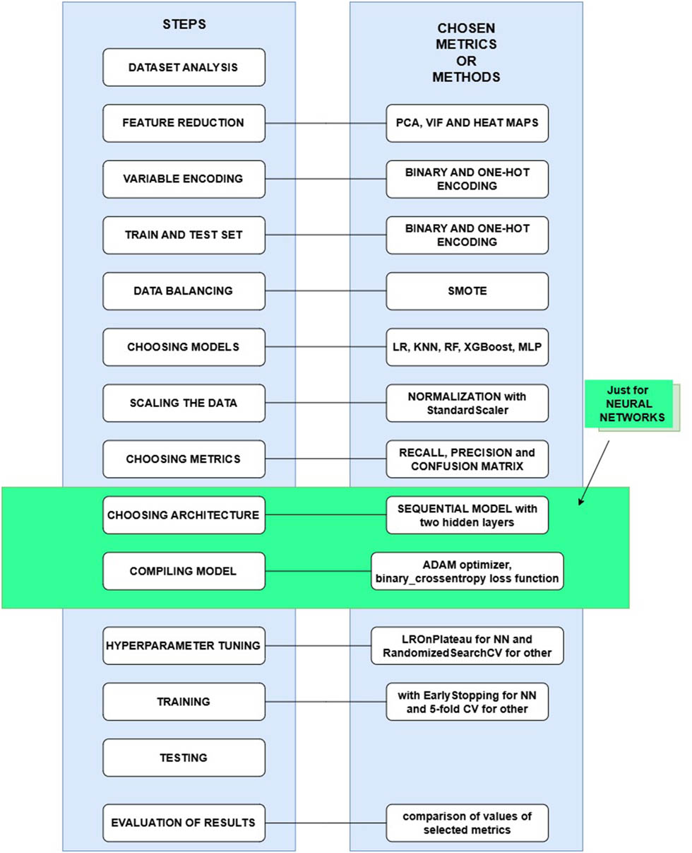
ML steps and chosen methods.
Only for MLP, it is particularly important to first choose the appropriate model architecture, as it directly affects the model’s performance and its ability to generalize. We did not experiment with different architectures, but based on reading the literature and the book by Chollet [42], a decision was made to choose the next architecture. A sequential model of the dense node type was chosen, consisting of an input layer with a number of nodes equal to the number of features in the dataset, followed by three hidden layers with 128, 64, and 32 nodes. A gradual decrease in the number of neurons in the network, i.e., dimensionality, helps the model to better classify the target variable. In this way, the model focuses on the features that were found to be significant in the previous layer. As an activation function, ReLU was used. ReLU introduces nonlinearity into deep learning models and addresses the issue of vanishing gradients. The last, the output layer, has one node, and we used sigmoid activation function, which is fast, simple, and used for binary classification. The MLP architecture is presented in Figure 6.

MLP architecture.
After choosing the architecture, the necessary step, only for MLP, is to compile the model. This means defining the loss function, so we selected binary_crossentropy (corresponds to binary classification and sigmoid), which measures how wrong the model estimates are compared to the actual values. For the optimizer, we selected adam, which minimizes the loss during training and updates the model’s weights. The selected metrics for MLP are precision and recall.
To adequately train all of these algorithms, a key step is to choose the best value of hyperparameters (hyperparameter tuning – HPT) of the selected models to create them. Hyperparameters are values that are adjusted before training and control the way the model “learns,” while parameters are values that the model itself “learns” during training. For traditional models, RandomizedSearchCV (RSCV) was used, instead of GridSearchCV, because it is less demanding and runs faster. Since the dataset is quite large, hyperparameter tuning requires a lot of time, so we resorted to stratified sampling and took 10% of the training data as a sample. The best parameter values were obtained over the sample, which will be further used when creating the model. For KNN, the hyperparameter k must be carefully selected, when k is small enough it can lead to overfitting to the training set, while too large k can make the classification imprecise. Also, the weights are an important hyperparameter. If its value is “uniform,” which is the default, all neighbors have equal importance, regardless of distance. If the value is “distance,” closer neighbors will have a greater influence on the decision [11]. When it comes to RF, hyperparameters, such as n_estimators (number of trees),max_depth (maximum tree depth), max_features (maximum number of features), and min_samples_leaf (minimum number of samples in a leaf), play a crucial role in optimizing model performance. These hyperparameters are carefully tuned to achieve better classification, but it is important to note that a larger number of trees may improve accuracy while also increasing processing time [18]. Some hyperparameters for XGBoost are n_estimators (the number of trees the model will create), learning rate (model adjustments with each iteration), subsample (fraction of samples used for each tree), and max_depth (it controls how deep each tree can grow) [19]. In the case of MLP, to adjust the parameter, i.e., the learning rate, ReduceLROnPlateau is used. The learning rate determines how quickly the model learns or how quickly the model adjusts its weights during training. If the learning rate is too low, it means the model will take a long time to converge, requiring many epochs to achieve good results. On the other hand, if this hyperparameter is set too high, it can lead to unstable learning and poor performance during classification [43].
The next step is to create models with the best parameters and train them on a scaled, balanced, entire training set (not on that sample). For traditional models, training and evaluation of the training set are conducted using the fivefold stratified CV. Since this is a large dataset, using more than fivefolds would be a lot. The values of the selected metrics obtained from the training evaluation represent the mean values calculated across the entire CV process. For MLP, instead of CV, we used “early stopping” with a patience parameter of 3, combined with the validation_split setting during training. The validation loss is monitored throughout training, and if it does not decrease over a certain number of epochs (determined by the patience parameter), the training process is automatically stopped. In each epoch, the model is trained on part of the training set (80%) and then evaluated on another part of the set (20%). Within each epoch, other tuples of the dataset are taken. The maximum number of epochs is set to 50, but thanks to “early stopping,” it can be stopped earlier.
The final step for all of these models is to check how the algorithm classifies new, unseen data and what the metric values are in that case. The new data are in a scaled, unbalanced test set. The obtained results will be presented in Section 4.
3.2.2 Second research phase
In this phase, we evaluated various architectures and configurations of the 1D CNN deep learning model to determine the best fit for our task. A prerequisite for the training and evaluation process of the 1D CNN model is the train–test split, as previously explained, while the remaining phases will be described in more detail.
The selected dataset, RTIoT2022, contains sequential data that can serve as input for CNN, especially in the form of a 1D CNN model. In this case, the input has a two-dimensional shape (numberOfFeatures, 1), where numberOfFeatures represents the number of features in the input data set, and 1 indicates the use of a single channel, meaning each feature value represents a measurement at a specific time [24]. In the following, various CNN models will be described, but evaluation results will be presented in Section 4.2.
3.2.2.1 CNN model 1
The complete architecture is provided in Figure 7. It consists of an input layer followed by three convolutional layers with 64, 128, and 256 applied filters, respectively. The kernel size (convolutional filter) for each layer is set to

CNN model 1 architecture.
3.2.2.2 CNN model 2
The architecture of model 2 is identical to the architecture of model 1, as shown in Figure 7. The difference between them lies in the data on which they are trained. Due to pronounced class imbalance in the dataset, for model 2, the SMOTE algorithm was applied, but in its enhanced version, Borderline-SMOTE. This method does not generate data randomly for the minority class, as regular SMOTE does, but uses KNN to identify samples that have neighbors from both classes – marked as “danger” – and uses these samples to generate new ones, thereby reducing noise in the data and preventing the generation of irrelevant samples [32]. This algorithm was chosen due to real-world challenges, where it is often difficult to distinguish between an attack and normal activity. Instead of using Borderline-SMOTE, an alternative approach is to assign different class weights during model training. For example, by increasing the weight of the minority class “0,” the model is encouraged to pay more attention to it and improve its recognition. This approach can contribute to better class balance.
3.2.2.3 CNN model 3
The architecture of model 3 is similar to the architecture of model 1, as shown in Figure 7, but with certain modifications. Specifically, in the second and third convolutional layers, the stride parameter was set to 2, while the kernel size was changed across layers:
3.2.2.4 CNN model 4
The architecture for model 4 has been modified and is shown in Figure 8. MaxPooling1D layers were removed after each convolutional layer and replaced with a single GlobalAveragePooling1D layer. This layer takes each feature map generated as output from the convolutional layers and, instead of passing all its values, computes the average value of all its elements. For example, if there are 64 feature maps, the output will be 64 average values – one for each feature map. These values are then used as input to the fully connected layer. Since GlobalAveragePooling1D already generates a one-dimensional vector, there is no need for an additional Flatten() layer. This reduces the amount of data and the computational load on the model because the model no longer needs to store all individual values from the feature maps, but only their average values. This reduces the dimensionality of the data, which can contribute to better model generalization, as redundant information is eliminated and the risk of overfitting is reduced [44].

CNN model 4 architecture.
3.2.2.5 CNN model 5
Model 5 is divided into models 5a and 5b. On top of the architectures of models 1 and 4, the ReduceLROnPlateau technique was applied, making them models 5a and 5b, respectively. In the previous models, the learning rate was set to
3.2.2.6 CNN model 6
Model 6 represents a deeper CNN architecture, as shown in Figure 9, by adding an additional convolutional layer with 512 nodes. The MaxPooling1D layer as well as dropout, batch normalization, and ReduceLROnPlateau, were retained.

CNN model 6 architecture.
4 Results
This article presents the results achieved through the previously described phases of model development: (i) the results of traditional architecture models ML methods (KNN, RF, XGBoost, and MLP) and (ii) the results of different CNN architectures applied to various versions of the initial dataset.
To enable a comparative analysis of the results, a BLM is introduced – a reference model that serves as a starting point for comparing the performance of more advanced models. The BLM defines the lower performance bound, showing the minimum level of efficiency a model must achieve to outperform solutions based on simpler architecture models.
4.1 First research phase
In the first phase, LR was selected as the reference model. In the second phase, when transitioning to 1D CNN models, the reference model becomes the best-performing model from the first phase, as it already provides an optimized solution among traditional models ML approaches.
The choice of LR as the reference model in the first phase is based on its simplicity and interoperability. Linear regression serves as a fundamental model that establishes the initial performance baseline and helps assess the improvements brought by more complex algorithms. LR trains quickly and enables fast result evaluation while providing insight into basic data trends before applying more advanced methods. As a rule, the hyperparameters of the BLM should not be optimized, but the default values should be used. Using the ROC curve, the ROC AUC value and applying Youden’s index, the optimal threshold for LR of 0.5 was obtained, which is also the default value.
The hyperparameters used during the development of the model in the first phase are shown in Table 4, which contains the following columns: chosen model, its selected parameters, the range of tested values for selected parameter, and the selected best value for the parameter. In addition, the value of F1-score for the selected parameters and performed HPT is also displayed. The value of only one metric can be obtained during HPT, so the F1-score was chosen.
Hyperpatameter values for ML models
| Model | Parameters | Possible values | Best value | Best score |
|---|---|---|---|---|
| KNN | n_neighbors | [5, 10, 15, 20] | 5 | 0.9929 |
| weights | [‘uniform’, ‘distance’] | distance | ||
| RF | n_estimators | [100, 300, 500] | 100 | 0.9957 |
| max_depth | [4, 6, 8] | 8 | ||
| max_features | [‘log2’, ‘sqrt’] | sqrt | ||
| min_samples _leaf | [1, 2, 4] | 2 | ||
| XGBoost | learning_rate | from 0.05 to 1.05 step 0.05 | 0,4 | 0.9967 |
| n_estimators | [100, 300, 500] | 300 | ||
| subsample | from 0.05 to 1.05 step 0.05 | 0.75 | ||
| max_depth | [4, 6, 8] | 4 | ||
| MLP | learning_rate | min is 0.001 | 0.001 | X |
In addition to hyperparameters, the RF algorithm also has the ability to calculate feature importance. Each feature has some significant value. In order to obtain a value of significance, it is first necessary to train the model, within the scope of this research using RSCV. A threshold of 0.0001 was determined and all features whose importance is greater than that threshold were extracted from the training set and used for training, testing, and evaluation of the RF model. Only 32 features were singled out, while many of them even have a feature importance equal to 0, and for that reason, the threshold is very low. In Figure 10, out of a total of 32 selected features, only 15 with the highest value for feature importance are shown, to make the graph clearer and more transparent. The target variable should not be used during feature importance.

RF feature importance.
Some of the factors in choosing the most suitable ML algorithm are times: (i) needed to find the hyperparameter values that give the best results, (ii) required for training the model using fivefold CV (over the entire training set), (iii) required for classic training of the model over the entire training set to evaluate the test set, and (iv) required for prediction for new, unclassified data.
In Table 5, the times are shown where the number in the column name corresponds to the number of the described time in the previous ordered list. With LR, there was no hyperparameter tuning, and for that reason, X value was set. The training and evaluation process is different at NN, and for that reason, the times are not in Figure 5. For this reason, the execution times for the MLP model are presented in Table 6.
Execution time for ML models development phases
| Model | 1 (s) | 2 (s) | 3 (s) | 4 (s) |
|---|---|---|---|---|
| LR | X | 47 | 9 | 0 |
| KNN | 22 | 227 | 0 | 40 |
| RF | 200 | 120 | 29 | 0 |
| XGBoost | 59 | 19 | 4 | 0 |
MLP phases execution times
| Time for model training | Time for evaluation on entire training set | Time for evaluation on entire test set | Time for model training | |
|---|---|---|---|---|
| MLP | X | 47 s | 9 s | 0 s |
During the evaluation, previously selected metrics are analyzed for each model separately. First, it is necessary to observe the performance for each model individually, i.e., metric values, separately for both training and test sets. If the values of the metrics are similar over both sets of data, it is concluded that there is no overfitting or underfitting. In a comparative analysis of two models, it is crucial to focus on the metric results over the test set for each model. The reference point in this analysis is the baseline algorithm. Tables 7 and 8 show the values of important metrics for each model separately.
ML model metric values for training set
| Training set | |||||
|---|---|---|---|---|---|
| 88487 positive i 88487 negative classes | |||||
| Recall | Precision | F1 score | FN | FP | |
| LR | 0.8613 | 0.9739 | 0.9141 | 12273 | 2042 |
| KNN | 0.9977 | 0.9920 | 0.9949 | 195 | 706 |
| RF | 0.9951 | 0.9991 | 0.9971 | 425 | 78 |
| XGBoost | 0.9966 | 0.9994 | 0.9980 | 298 | 49 |
| MLP | 0.9965 | 0.9908 | 0.9937 | 308 | 811 |
ML model metric values for test set
| Test set | |||||
|---|---|---|---|---|---|
| 2501 positive i 22123 negative classes | |||||
| Recall | Precision | F1 score | FN | FP | |
| LR | 0.8559 | 0.9979 | 0.9215 | 3187 | 40 |
| KNN | 0.998 | 0.9988 | 0.9984 | 44 | 26 |
| RF | 0.9948 | 0.9995 | 0.9972 | 114 | 10 |
| XGBoost | 0.9966 | 0.9996 | 0.9981 | 76 | 9 |
| MLP | 0.9954 | 0.9985 | 0.9736 | 101 | 33 |
4.2 Second research phase
All the 1D CNN models described in the previous section were first trained and evaluated on the raw dataset (RTIoT2022), without any preprocessing. The reason for this is to select the best 1D CNN models for our problem. Additionally, it is recommended that CNN models do not require extensive raw data preparation, which we will verify by analyzing the results presented in the following article. Obtained result only on raw, RTIoT2022 dataset is discussed in this section.
4.2.1 CNN model 1
Model 1 was initially trained and evaluated on the raw dataset (RTIoT2022). Without data scaling, we noted a high error rate during the training process, suggesting that the model was unable to adequately capture patterns in the data. Additionally, the precision metric was lowered, indicating that the model was not classifying positive instances (representing attacks) well enough. Due to these observed issues, data scaling became essential for all the models described further. The StandardScaler method was chosen, as in the first phase.
Then, the scaled, but imbalanced dataset was used for training and evaluation. However, there is a significant imbalance between attacks and normal activities; in our case, there are more attacks, so the model may become overly biased toward labeling everything as an attack (leading to more FP). This way, the model becomes biased toward the majority class and fails to recognize the minority class.
The final decision was to avoid using such a model architecture combined with raw and imbalanced data.
4.2.2 CNN model 2
An alternative approach for data balancing was initially attempted, where class weights were manually adjusted. However, in our case, this method did not yield satisfactory results, as confirmed by the confusion matrix analysis. The reason for this was the improper setting of the weights, which compromised the model’s classification ability. For this reason, the architecture of model 2, combined with the application of Borderline-SMOTE on the raw dataset (RTIoT2022), produced satisfactory results as shown in Tables 10 and 11, and this model will be analyzed on other versions of the dataset as well.
CNN model metric values for training set
| TRAINING SET – 88487 positive and 88487 negative classes | |||||||
|---|---|---|---|---|---|---|---|
| CNN architecture | Dataset | Recall | Precision | F1 score | Loss | FN | FP |
| Model 2 | RTIoT2022 | 0.992453 | 0.998124 | 0.995280 | 0.091889 | 433 | 25 |
| RTIoT2022-v2 | 0.998217 | 0.997187 | 0.997702 | 0.092522 | 40 | 2 | |
| RTIoT2022-v3 | 0.996806 | 0.998216 | 0.997511 | 0.093601 | 179 | 0 | |
| RTIoT2022-v4 | 0.998106 | 0.999151 | 0.998628 | 0.073247 | 34 | 41 | |
| Model 3 | RTIoT2022 | 0.992396 | 0.997684 | 0.995033 | 0.087543 | 352 | 210 |
| RTIoT2022-v2 | 0.997046 | 0.998118 | 0.997582 | 0.071861 | 47 | 2 | |
| RTIoT2022-v3 | 0.997555 | 0.998755 | 0.998154 | 0.069801 | 34 | 41 | |
| RTIoT2022-v4 | 0.997343 | 0.998401 | 0.997872 | 0.061713 | 122 | 0 | |
| Model 4 | RTIoT2022 | 0.990658 | 0.997524 | 0.994079 | 0.118748 | 345 | 870 |
| RTIoT2022-v2 | 0.997442 | 0.998260 | 0.997851 | 0.102647 | 256 | 4 | |
| RTIoT2022-v3 | 0.998191 | 0.999024 | 0.998607 | 0.100076 | 41 | 2 | |
| RTIoT2022-v4 | 0.998262 | 0.999024 | 0.998643 | 0.084411 | 98 | 1 | |
| Model 5 | RTIoT2022 | 0.994262 | 0.998566 | 0.996409 | 0.019771 | 262 | 35 |
| RTIoT2022-v2 | 0.992014 | 0.997017 | 0.994509 | 0.101706 | 518 | 46 | |
| RTIoT2022-v3 | 0.996778 | 0.998343 | 0.997559 | 0.093860 | 128 | 9 | |
| RTIoT2022-v4 | 0.997951 | 0.998826 | 0.998388 | 0.081147 | 18 | 4 | |
CNN model metric values for test set
| TEST SET – 17661 positive and 17734 negative classes | |||||||
|---|---|---|---|---|---|---|---|
| CNN architecture | Dataset | Recall | Precision | F1 score | Loss | FN | FP |
| Model 2 | RTIoT2022 | 0.993854 | 0.999773 | 0.995280 | 0.048881 | 128 | 4 |
| RTIoT2022-v2 | 0.998590 | 1 | 0.999295 | 0.039975 | 25 | 3 | |
| RTIoT2022-v3 | 0.999041 | 0.999943 | 0.999492 | 0.039846 | 47 | 1 | |
| RTIoT2022-v4 | 0.998478 | 1 | 0.999238 | 0.034261 | 60 | 0 | |
| Model 3 | RTIoT2022 | 0.993910 | 0.999829 | 0.996861 | 0.060166 | 124 | 55 |
| RTIoT2022-v2 | 0.999211 | 1 | 0.999605 | 0.016835 | 17 | 1 | |
| RTIoT2022-v3 | 0.999943 | 0.999718 | 0.999831 | 0.009511 | 15 | 13 | |
| RTIoT2022-v4 | 0.996842 | 1 | 0.998419 | 0.032076 | 56 | 0 | |
| Model 4 | RTIoT2022 | 0.994756 | 0.990386 | 0.992566 | 0.359166 | 102 | 237 |
| RTIoT2022-v2 | 0.999267 | 1 | 0.999633 | 0.077863 | 86 | 0 | |
| RTIoT2022-v3 | 0.999549 | 1 | 0.999774 | 0.032988 | 24 | 1 | |
| RTIoT2022-v4 | 0.999098 | 1 | 0.999549 | 0.026980 | 39 | 0 | |
| Model 5 | RTIoT2022 | 0.995151 | 0.999773 | 0.997457 | 0.019199 | 86 | 10 |
| RTIoT2022-v2 | 0.993797 | 0.999374 | 0.996578 | 0.049606 | 166 | 11 | |
| RTIoT2022-v3 | 0.997181 | 1 | 0.998588 | 0.046900 | 50 | 4 | |
| RTIoT2022-v4 | 0.998985 | 1 | 0.999492 | 0.030874 | 18 | 4 | |
4.2.3 CNN model 3
For model 3, the raw RTIoT2022 dataset was used with Borderline-SMOTE applied, which is in line with previous conclusions. However, this architecture led to an increased number of FP and FN in the confusion matrix. Results are shown in Tables 10 and 11. It is possible that the change in kernel size and stride parameters caused a loss of key information, making it harder for the model to learn complex patterns in the data. It may have been necessary to properly preprocess and clean the data beforehand, which is why model 3 was chosen for further analysis.
4.2.4 CNN model 4
Model 4, applied to the raw but balanced RTIoT2022 dataset, resulted in a slightly higher loss but achieved good precision and recall values, so it was decided to further test it on the remaining datasets described in the Section 3.1.
4.2.5 CNN model 5
The application of this method slowed down training because it adjusts the learning rate based on metric values, in our case, the validation loss. Although ReduceLROnPlateau provided very similar results to when it was not used, it should still be included in the model training process. The reason for this is the more stable model learning on the provided dataset, as the hyperparameter is adjusted automatically. Also, if there is no reduction in validation loss over several epochs, the learning rate can be decreased to allow the model to learn more complex patterns without wasting training resources without improving performance.
4.2.6 CNN model 6
Model 6 was tested on the balanced RTIoT2022 dataset. The model evaluation resulted in a large number of FN in the confusion matrix, which is not desirable for ANIDS systems, as this number should be minimized. It was concluded that a simpler architecture yielded better results, and therefore, it does not need to be deepened. Also, this model will not be tested on the other versions of the dataset for the same reason.
After analyzing all the models on the raw RTIoT2022 dataset, it was concluded that models 2–5 perform well, and it was decided to further test and evaluate them on the remaining datasets. Remaining datasets are RTIoT2022-v2, RTIoT2022-v3, and RTIoT2022-v4. An overview of these models is presented in Table 9.
Overview of CNN architectures
| Model | Architecture | BorderLine-SMOTE | Model compile parameters | ReduceLROn-Plateau | Model training parameters |
|---|---|---|---|---|---|
| Model 2 | Figure 7 | Yes | Optimizer: Adam loss: binary_crossentropy metrics: precision, recall, F1-score, confusion matrix | No | epochs: 30 batch_size: 64 earlystopping: patience 3 |
| Model 3 | X | Yes | No | ||
| Model 4 | Figure 8 | Yes | No | ||
| Model 5 | X | Yes | Yes |
In Tables 10, as in Table 11, we can see the results of the selected metrics over the training and test data of each experiment. There were a total of 16 experiments because each selected model was trained and evaluated on all versions of the dataset presented in Section 3.1. There are results for the raw RTIoT2022, too. A discussion of the results of applying the selected models to other versions of the dataset (RTIoT2022-v2, RTIoT2022-v3, and RTIoT2022-v4) can be found in Section 5.
5 Discussion
In order to select one of the presented models, it is important to take into account all the aforementioned results. Within this section, the authors’ observations and guidelines for further development and improvement of the conducted research are given. For better understanding, the key items will be discussed in chronological order, following the flow of the research.
When we talk in the context of models developed within the scope of the first phase, the execution time of the various stages in ML model development plays a very important role in the overall efficiency of the process. For this reason, when selecting the best model, it is important to focus on its performance when it comes to execution time. Choosing a model that achieves a balance between high metric results and time efficiency can significantly contribute to successful implementation in real-world conditions, where reaction time is often critical.
Conclusions about the speed of the developed models were made by analyzing the times required for different phases, as shown in Table 5. When it comes to finding hyperparameters as well as the time required for model training, the best results are observed with the KNN model. For model training, XGBoost also achieves very good results, which is also much better than KNN when it comes to predicting new hacker attacks. The performance of the MLP model is average, while the RF shows a much weaker performance in both aspects. It is important that the training process is efficient in order to learn the algorithm quickly, but equally important is how quickly the model can make predictions. Faster predictions allow the system to detect potential attacks faster, which is critical for timely response to real-time threats. For these reasons, we conclude that in terms of execution speed, XGBoost takes the lead.
In order to check whether the models are overfitted or underfitted, a comparative analysis of the metrics obtained over the training and test set is performed. Given that the values of the metrics, as shown in Tables 7 and 8, are similar in both datasets, it is concluded that developed models are neither overfitted nor underfitted. This means that models are capable of handling unknown data well, without being overadapted to the specifics of the training set.
XGBoost proved to be the model with the highest evaluation precision on the training set. Due to small differences in the results of the metrics, the F1-score was also considered, which additionally confirms the advantage of this model compared to others. It is particularly important how the model classifies instances that indicate a hacker attack, i.e., how often it misclassifies a positive instance as a negative one, which is crucial to avoid. This situation was analyzed through the FNP metric, where KNN achieved the best results, while XGBoost was just behind. On the other hand, the FPR, which measures the number of normal activities mistakenly classified as hacker attacks, is also important. In this respect, XGBoost significantly stands out as the best, while KNN performs significantly poorly on this metric. When considering the test set, which is crucial for performance evaluation, KNN and XGBoost again stand out as the best-performing models. It is particularly significant that XGBoost shows a minimal difference in F1-score between the training and test sets, indicating the stability and consistency of the model in classifying instances.
Unlike the first phase, where we discussed the time required for different stages of ML model development, the discussion about the second phase will not focus on execution time. The main reason is the clear advantage of traditional models in terms of speed, as CNN models have a different architecture and data processing approach compared to KNN, RF, XGBoost, and MLP models. These models work with feature vectors, while CNN processes sequential data, making it difficult to directly compare training/testing times between them.
In the second phase, the focus is on evaluating how different configurations affect metric results, while time analysis will become relevant in later stages of model optimization. After selecting the architecture that achieves the highest accuracy and precision in classifying instances, further work will involve analyzing and optimizing training and testing times.
The model evaluation is based on key metrics that enable a comprehensive analysis of its accuracy, generalization ability, and effectiveness in anomaly detection. Following are the conclusions drawn from the results presented in Section 4.
The first, and somewhat unexpected, conclusion is that the original dataset did not yield the best results on any of the developed models. Why is this unexpected? Because CNN models typically do not require extensive preprocessing, they have the ability to automatically extract relevant features from the data. However, in the case of network traffic, additional data processing can be crucial for improving model performance. Additionally, we can observe that the results vary significantly depending on the version of dataset used for training and testing. This justifies exploring different preprocessing techniques to identify the combination that yields the best results.
When analyzing the results, we examine the confusion matrix along with FP and FN. FN is generally more dangerous because actual attacks go undetected, which can have serious security consequences. FP can be frustrating as it triggers false alarms, but it does not directly compromise security.
Considering this, among all the presented model and dataset version combinations, and evaluating both the training and testing phases, the combinations that achieve the best results are as follows:
CNN model 3 on the RTIoT2022-v2 dataset version and
CNN model 5 on the RTIoT2022-v4 dataset version.
Although model 3 demonstrates slightly better performance in the testing phase, there is a noticeable difference between its corresponding training and testing results, which may indicate overfitting. In contrast, model 5 exhibits more stable performance, with significantly smaller variations between training and testing results.
For these reasons, the final conclusion is that the most successful model in the second research phase is model 5, 1D CNN developed using the RTIoT2022-v4 dataset. This dataset was obtained by applying the Winsorization technique to handle outliers and using PCA, VIF, and Pearson’s test for feature selection.
As previously mentioned, the BLM for the second phase is the model that achieved the best performance in the first development phase, which in this case is the XGBoost model. To support the final decision, Table 12 contains the key evaluation metrics that allow for a direct comparison of the selected models: recall, precision, and F1-score. Based on these values, we conclude that deep learning, specifically the 1D CNN architecture referred to as “model 5,” offers the best results when using a dataset that has undergone dimensionality reduction and outlier handling.
Evaluation metrics for XGBoost and CNN “model 5”
| Model | Dataset | Recall | Precision | F1 score |
|---|---|---|---|---|
| Training set | ||||
| XGBoost | RTIoT2022 | 0.9966 | 0.9994 | 0.998 |
| CNN model 5 | RTIoT2022-v4 | 0.997951 | 0.998826 | 0.998388 |
| Test set | ||||
| XGBoost | RTIoT2022 | 0.9966 | 0.9996 | 0.9981 |
| CNN model 5 | RTIoT2022-v4 | 0.998985 | 1.000000 | 0.999492 |
6 Proposed enhancements for the ML model
In this section, we will discuss potential methods for evaluating ML model explainability, testing the developed model on different datasets, and exploring possible strategies for model optimization.
6.1 Model explainability
The selected ML model, “model 5,” achieves high accuracy in predictions, but the explainability of its decisions remains an open question. Explainable Artificial Intelligence (XAI) aims to make ML algorithm decisions transparent and understandable, rather than leaving them hidden within a “black box” [45]. It is crucial to determine whether the model’s decisions are unbiased and based on relevant factors. Potential issues include biases due to imbalanced data, overconfidence in incorrect predictions, and a lack of insight into the key features that influenced the decision [45]. For example, if the system marks certain traffic as an attack, network administrators must understand the reasoning behind that decision to respond appropriately and improve security policies.
For these reasons, the next step in the research focuses on examining why and how the selected CNN model makes its decisions. This enhances trust in the model and, based on improvements derived from these insights, enables better practical decision-making.
XAI encompasses a set of techniques that visualize the key features influencing an ML model’s decisions. By analyzing these visualizations, domain experts can assess whether the model’s decisions are logical and aligned with real-world expectations.
To provide clear and understandable insights into how the proposed NIDS operates, the idea is to assess model explainability using SHapley Additive Explanations (SHAP), Local Interpretable Model-agnostic Explanations (LIME), and Layer-wise Relevance Propagation (LRP).
Since the selected model belongs to the CNN family, it is important to note that most XAI methods applied to CNNs are designed for image-based inputs, whereas the chosen model is trained on sequential tabular data. In this case, special attention must be given to adapting the input format for XAI methods to ensure a meaningful analysis and achieve optimal results. This requires a thorough review of prior research addressing similar challenges.
This article presents the results of applying the SHAP method to explain the selected 1D CNN model (“model 5”) trained on sequential data. This marks the beginning of research in this direction, with future work focused on integrating LIME and LRP techniques, followed by a comparative analysis of the insights obtained from SHAP values.
These techniques can also contribute to model optimization by allowing training on a reduced set of features identified as the most influential through XAI analyses. The most impactful features are extracted and used to train new classifiers to evaluate whether they can achieve the same or better performance compared to models trained on the full feature set.
This approach helps assess how truly relevant the selected features are for the model’s decision-making. If they yield satisfactory results, the model becomes optimized, as it operates on a smaller input set. One of the conclusions from the study by Ullah et al. [45] indicates that, in their proposed system, this method enhances performance in terms of accuracy, precision, F1-score, and computation time. Additionally, it significantly reduces the number of features required in the deployed system, which is crucial for resource-constrained environments, such as edge devices.
Furthermore, in the context of comprehensive system optimization, it is essential to consider the computational complexity of XAI technologies, especially since the proposed system is intended for real-time decision-making. These optimization strategies represent the next research steps, with the results planned for presentation in future studies building upon the results presented in this article.
The SHAP method enables the examination of individual feature contributions to software defect prediction, promoting transparency and interoperability [46]. The architecture incorporating this method, applied to the 1D CNN model (“model 5”), is illustrated in Figure 11. Its implementation builds upon previous research phases and is conducted using an ML model trained on a designated portion of the dataset for training. The trained model is utilized by the SHAP technique to visualize the most important features [46]. In addition to training data, the test set is used to evaluate the consistency and robustness of the identified features on unseen data. By analyzing SHAP values on the test set, we can determine whether the model maintains the same classification patterns for network traffic, ensuring its generalization and reliability in real-world scenarios.

ML model explainability using the SHAP method.
Using the generated visualizations, a subset of features is identified as the most relevant for distinguishing between normal network traffic and traffic indicative of a cyberattack.
Figure 12 presents the results of the SHAP analysis applied to the selected model.

SHAP analysis of the most influential features.
The features are ranked by importance, with down_up_ratio being the most influential in the model’s decision making. Other significant features include flow_SYN_flag_count, flow_pkts_per_sec, and proto_icmp, suggesting that the model relies on a combination of protocol types, flag counts, packet rates, and traffic distribution for classification.
Each point on the graph represents an individual instance from the test set. Blue points indicate the low feature values, while red points indicate the high feature values. The position of the points along the
A comparative analysis of the graph from Figure 12 and the descriptive statistics of the most influential features led to conclusions about the explainability of the selected ML model, and summarized in Table 13.
Descriptive statistics and analysis of the most influential features
| down_up_ratio | flow_SYN_ flag_count | flow_pkts_ per_sec | proto_icmp | payload_bytes_ _sec | ||
|---|---|---|---|---|---|---|
| Descriptive statistics | min | 0 | 0 | 0 | 0 | 0 |
| max | 6.08 | 8 | 2097152 | 1 | 125829120 | |
| mean | 0.85 | 0.95 | 703568.28 | 0.0004629 | 41053451.79 | |
| std | 0.34 | 0.47 | 741563.42 | 0.0215119 | 44857059.62 | |
| Feature interpretation | It represents the ratio of downloaded to uploaded data. For example, a value of 6 means downloaded data is six times greater than uploaded. A higher ratio doesn’t always indicate an attack. For example, in DDoS attacks, the goal is to overwhelm a server with excessive traffic, increasing downloaded data while the attackers send minimal data. | A high number of SYN flags may indicate port scanning or a SYN flood attack, both of which are forms of DoS attacks. However, under normal conditions, SYN flags are a typical characteristic of TCP communication. | The packet transmission rate can be a crucial indicator of an attack, especially if it is unusually high and deviates from typical network traffic patterns. | Although ICMP packets are part of normal network traffic, an unusual number or patterns of these packets may indicate potential malicious activity. | This metric measures the amount of data (in bytes) transmitted per second, which can provide valuable insights into unusual or malicious activities within the network. | |
| Feature analysis | A maximum value of 6.08 indicates that, in some cases, the amount of downloaded data significantly exceeds the uploaded data. Given that the average value is 0.85 with a relatively small standard deviation (0.34), values considerably above the average may represent anomalies and serve as potential indicators of attacks. | A maximum value of 8 indicates the presence of traffic flows with a very high number of SYN flags, which may suggest a potential attack. Given that the average value is 0.95, instances with values close to the maximum are significantly above the usual range and warrant further attention | A maximum value of 2.09 million packets per second indicates extremely high traffic in certain cases. The average value of 703 568, combined with a high standard deviation (741563), suggests significant variations, highlighting the need for a detailed analysis of flows with extreme values. | A maximum value of 1 indicates the presence of ICMP packets, but the average value of 0.00046 suggests that such packets are rare. This further emphasizes that in the analyzed network structure, ICMP traffic may be used for covert attacks. | A maximum value of 125.8 million bytes per second suggests potential network overload. Given the high average load (41 million bytes per second) and a standard deviation of 44.8 million, extreme values may indicate an attack involving large volumes of data (such as DDoS or data exfiltration). | |
Based on the interpreted results, it can be concluded that the model successfully identifies the characteristics specific to network attacks. To further validate these findings, the model could be trained and tested on a dataset with a reduced feature set, which is also planned as one of the future improvements of this study.
6.2 Expanding model validation
Another approach that can contribute to increased trust in model decisions is testing the proposed architecture on different datasets. As identified in the literature review, there are several publicly available datasets collected from the network infrastructure of IoT devices.
To ensure that the analysis of model performance on new datasets is comparable to the initial dataset, it is first necessary to verify whether their granularity aligns. In cases of mismatch, if feasible, the granularity of the new datasets should be adjusted to maintain consistency. Subsequently, feature mapping must be performed to align features with different names, followed by data standardization or normalization to ensure a uniform scale. Finally, preprocessing should be conducted in the same manner as with the initial dataset before testing the selected ML model.
If the model exhibits similar performance across different but thematically related datasets, this indicates its generalization ability and reduces the likelihood of overfitting to the specific characteristics of the initial dataset. Utilizing multiple datasets enhances the credibility of the results, demonstrating that the model does not perform well solely on a single dataset but maintains consistency and reliability under various experimental conditions.
Beyond performance evaluation, an additional step toward increasing trust in the model is analyzing its interpretability using XAI techniques. If key features identified in the initial dataset also emerge as the most influential in other datasets, this may indicate that the model relies on universal patterns for decision-making rather than on dataset-specific or random factors.
Incorporating multiple datasets into model evaluation not only strengthens the reliability of the results but also enables a deeper analysis of interpretability, potential biases, and the robustness of learned patterns. By combining testing on different datasets and XAI analysis, confidence in the model’s decisions can be further reinforced.
Although the implementation of these methods is beyond the scope of the current study, they represent important directions for future research. The proposed approach would enable a more comprehensive validation of the model and enhance its applicability in real-world network traffic scenarios involving IoT devices.
6.3 Possible CNN model optimizations: lightweight architectures, pruning, and quantization
The 1D CNN architecture (referred to as “model 5”) has been chosen as the most suitable model for attack detection in the IoT environment. The model was trained and evaluated on the RT-IoT2022-v4 dataset. One of the possible approaches to implementing the NIDS system is deploying it on edge devices (such as Raspberry Pi, Jetson Nano, and Intel NUC), which enable local traffic analysis. Raspberry Pi, for example, is a compact computer that is often connected to the IoT network with the goal of collecting data and potential attack detection. However, applying a CNN model to these devices presents a challenge due to limited resources, which may lead to increased battery, memory, and processing resource consumption, longer training and prediction times, and higher operational costs. To overcome these obstacles, optimizing CNN models to achieve greater computational efficiency is crucial.
The optimization so far has included reducing the number of layers and neurons, as well as applying dropout to prevent overfitting. Training on cloud infrastructure has enabled seamless data processing, but if edge IoT devices were used in the future, computational efficiency would remain a challenge. For this reason, two additional optimization approaches are being considered, which will be the subject of future research. One approach is the use of lightweight models based on CNN architecture, adapted for operation on IoT devices. These architectures enable faster traffic analysis, scalability, and lower latency by reducing the number of learning parameters and computational complexity. However, their application may negatively affect accuracy, particularly metrics such as precision and recall. Although architectures such as MobileNet[9], ShuffleNet[10], SqueezeNet[11], and EfficientNet[12], were originally developed as lightweight 2D CNN models for image processing, an attempt to adapt them to 1D CNN architectures could be one of the next steps of our research.
The second approach to CNN model optimization involves pruning and quantization techniques, which enable more efficient model application on IoT devices with limited resources. Pruning eliminates unnecessary and redundant parameters, reducing the overall model size and adapting the architecture to the specifics of IoT devices. Quantization lowers the precision of weights and activation functions by converting floating-point values into 8-bit or lower integer values, significantly reducing memory and energy consumption. Although both methods improve efficiency, finding the right balance is necessary, as excessive optimization may reduce model accuracy and its ability to learn complex patterns. By carefully combining pruning and quantization, an optimal trade-off between computational cost and model accuracy can be achieved [47].
The conceptual proposal for future research involves adapting the mentioned lightweight models to our use case and comparing the number of parameters, training and prediction times, and computational requirements with the CNN architectures presented in this article. Additionally, pruning and quantization techniques can be applied to all models, followed by a comparative analysis of the obtained results. This would allow a detailed examination of the trade-off between reduced computational cost and potential accuracy degradation. The best model can be implemented and deployed on a Raspberry Pi device using lightweight frameworks such as TensorFlow Lite[13] or PyTorch[14], enabling the evaluation of its real-world performance in a constrained IoT environment.
7 Conclusion
Through the analysis of all models across two research phases, it was concluded that XGBoost delivered the best results in the first phase, striking a balance between accuracy and execution speed, making it an ideal choice for real-world IDS applications. In the second phase, which focused on deeper architectures, CNN model 5 demonstrated the most stable performance on the RTIoT2022-v4 dataset. Although CNN model 3 achieved slightly better test results, signs of potential overfitting were observed, whereas CNN model 5 maintained consistency between training and test sets.
The final selection for the best model in the second phase is CNN model 5, which utilized enhanced data processing techniques, including Winsorization for outlier handling and feature selection methods, ensuring optimal accuracy and generalization.
A comparative analysis of the top-performing models from both phases led to the conclusion that the developed neural network holds a clear advantage. Therefore, the final chosen model is CNN model 5.
To ensure trust in the decisions made by the ML model, the explainability of the predictions was verified using the SHAP method. In Section 6.1, we presented a discussion on various XAI techniques and gave suggestions for future directions regarding model explainability.
It is important to emphasize that execution time was not a determining factor in the final selection. This phase of research leaves gap for future improvements, particularly in optimizing the selected model to further enhance its efficiency, as described in Section 6.3.
With the implementation of the presented ML model and its integration within a real-time IDS system, the possibility of detecting potential hacker attacks is expected based on the values of selected attributes of devices and messages that participate in communication. The algorithm that will detect such attacks is the first step in the process of ensuring secure communication.
An additional direction for future research involves developing a dataset that simulates network traffic under the conditions defined in this study. Given that cyber attacks are constantly evolving, adapting, and improving to evade IDS systems, it is crucial for models designed for ANIDS solutions to keep pace with these trends and continuously learn from new data. This would ensure the protection of IoT devices against an increasingly diverse range of attacks. In particular, creating a dataset based on data from IIoT devices within an Industry 4.0 network would be highly beneficial, enabling further analysis of the developed model’s applicability in this context.
Acknowledgments
The authors are grateful for the reviewer’s valuable comments that improved the manuscript.
-
Funding information: This research was supported by the Ministry of Science, Technological Development and Innovation (Contract No. 451-03-137/2025-03/200156) and the Faculty of Technical Sciences, University of Novi Sad through Project “Scientific and Artistic Research Work of Researchers in Teaching and Associate Positions at the Faculty of Technical Sciences, University of Novi Sad 2025” (No. 01-50/295).
-
Author contributions: All authors have accepted responsibility for the entire content of this manuscript and consented to its submission to the journal, reviewed all the results, and approved the final version of the manuscript.
-
Conflict of interest: The authors state no conflict of interest.
-
Data availability statement: The dataset analyzed during the current study is available in the UC Irvine Machine Learning Repository.
References
[1] K. Brunel Rolack and A. Mehdi, “Machine learning-based intrusion detection methods in IoT systems: A comprehensive review,” Electronics, vol. 13, no. 18, p. 3601, 2024. 10.3390/electronics13183601Search in Google Scholar
[2] A. Lazarevic, L. Ertoz, V. Kumar, A. Ozgur, and J. Srivastava, “A comparative study of anomaly detection schemes in network intrusion detection,” in: Proceedings of the Third SIAM International Conference on Data Mining, May 2003, pp. 25–36. 10.1137/1.9781611972733.3Search in Google Scholar
[3] M. Imad, M. Hassan, S. Bangash, and N. Naim, “A comparative analysis of intrusion detection in IoT network using machine learning,” in: Big Data Analytics and Computational Intelligence for Cybersecurity, Springer Nature, Cham, Switzerland, Sep 2022, pp. 149–163. 10.1007/978-3-031-05752-6_10Search in Google Scholar
[4] E. E. Abdallah, W. Eleisah, and A. F. Otoom, “Intrusion detection systems using supervised machine learning techniques: a survey,” in: The 13th International Conference on Ambient Systems, Networks and Technologies (ANT), vol. 201, no. C. Elsevier B.V., Porto, Portugal, March 2022, pp. 205–212. .https://doi.org/10.1016/j.procs.2022.03.029. Search in Google Scholar
[5] N. Moustafa and J. Slay, “Unsw-nb15: a comprehensive data set for network intrusion detection syst. (unsw-nb15 network data set),” in: 2015 Military Commun. and Inf. Syst. Conf., MilCIS 2015 - Proc., Nov 2015. 10.1109/MilCIS.2015.7348942Search in Google Scholar
[6] E. Hodo, X. Bellekens, A. Hamilton, P. L. Dubouilh, E. Iorkyase, and C. Tachtatzis, “Threat analysis of IoT networks using artificial neural network intrusion detection system,” in: 2016 International Symposium on Networks, Comput. and Commun., ISNCC 2016, 2016, pp. 4–8. 10.1109/ISNCC.2016.7746067Search in Google Scholar
[7] I. Mutambik, “An efficient flow-based anomaly detection system for enhanced security in IoT networks,” Sensors, vol. 24, no. 22, 7408, 2024. 10.3390/s24227408Search in Google Scholar PubMed PubMed Central
[8] O. D. Jovanović, Early discovery of the devices infected with botnetmalware using network flow anomaly detection, Ph.D. dissertation, University of Belgrade, Belgrade, 2024. Search in Google Scholar
[9] V. Karanam, “Is there a Trojan!: Literature survey and critical evaluation of the latest ML based modern intrusion detection systems in IoT environments,” Int. J. Cybernet. Inform., vol. 12, no. 3, pp. 67–87, 2023. 10.5121/ijci.2023.120306Search in Google Scholar
[10] D. Gladic, J. Petrovacki, S. Sladojevic, M. Arsenovic, and S. Ristic, “IDS-based Machine Learning model specific for secure data transmission within the frame of IoT network infrastructure,” in: 2024 IEEE 17th International Scientific Conference on Informatics (Informatics), Poprad, Slovakia, Nov 2024, pp. 75–81. 10.1109/Informatics62280.2024.10900811Search in Google Scholar
[11] G. Guo, H. Wang, D. A. Bell, Y. Bi, D. Bell, and K. Greer, “Knn model-based approach in classification,” in: On The Move to Meaningful Internet Systems 2003: CoopIS, DOA, and ODBASE, ser. Lecture Notes in Computer Science, R. Meersman, Z. Tari, and D. C. Schmidt, Eds., vol. 2888, Springer, Berlin, Heidelberg, 2003, pp. 986–996. https://doi.org/10.1007/978-3-540-39964-3_62. Search in Google Scholar
[12] S. Strecker, W. Haaften, and R. Dave, “An analysis of IoT cyber security driven by machine learning,” in: Proc. of Int. Conf. on Commun. and Comput. Technologies, Springer Nature, Cham, Switzerland, Jan 2021, pp. 725–753. 10.1007/978-981-16-3246-4_55Search in Google Scholar
[13] S. N. B. S. Sham, K. K. Ishak, N. A. M. Razali, N. M. Noor, and N. A. Hasbullah, “IoT attack detection using machine learning and deep learning in smart home,” Int. J. Inform. Visualization, vol. 8, no. 1, pp. 510–519, 2024. 10.62527/joiv.8.1.2174Search in Google Scholar
[14] A. Presciuttini, A. Cantini, F. Costa, and A. Portioli-Staudacher, “March, Machine learning applications on IoT data in manufacturing operations and their interpretability implications: A systematic literature review,” J. Manuf. Syst., vol. 74, pp. 477–486, 2024, https://doi.org/10.1016/j.jmsy.2024.04.012. Search in Google Scholar
[15] S. Sperandei, “Understanding logistic regression analysis,” Biochem. Med., vol. 24, no. 1, pp. 12–18, 2014. 10.11613/BM.2014.003Search in Google Scholar PubMed PubMed Central
[16] V. Kecman, “Support vector machines - an introduction,” in: Studies in Fuzziness and Soft Comput., vol. 177, Springer, Berlin, April 2005, pp. 1–47. 10.1007/10984697_1Search in Google Scholar
[17] treeplan.com, Introduction to decision trees, https://treeplan.com/wp-content/uploads/introduction-to-decision-trees.pdf, n.d., accessed: 2025-02-19. Search in Google Scholar
[18] L. Breiman, “Random Forests,” Mach. Learning, vol. 45, no. 1, pp. 5–32, 2001. 10.1023/A:1010933404324Search in Google Scholar
[19] M. A. O. Ahmed, Y. AbdelSatar, R. Alotaibi, and O. Reyad, “Enhancing Internet of Things security using performance gradient boosting for network intrusion detection systems,” Alexandria Eng. J., vol. 116, December 2024, pp. 472–482, 2025. https://doi.org/10.1016/j.aej.2024.12.106. Search in Google Scholar
[20] A. Ali, M. Assam, F. U. Khan, Y. Y. Ghadi, Z. Nurdaulet, A. Zhibek, et al., “An optimized multilayer perceptron-based network intrusion detection using gray wolf optimization,” Comput Elect. Eng., vol. 120, pp. 100947–100966, 2024, https://doi.org/10.1016/j.compeleceng.2024.109838. Search in Google Scholar
[21] S. Balamurugan “A comprehensive study on MLP and CNN, and the implementation of multi-class image classification using deep CNN,” in: Machine Learning and Deep Learning Techniques for Medical Science, CRC Press, London, United Kingdom, 2022, pp. 1–25. 10.1201/9781003217497-1Search in Google Scholar
[22] A. Arul Anitha and L. Arockiam, “ANNIDS: Artificial neural network based intrusion detection system for internet of things,” Int. J. Innovative Technol. Exploring Eng., vol. 8, no. 11, pp. 2583–2588, 2019. 10.35940/ijitee.K1875.0981119Search in Google Scholar
[23] J. Kim, J. Kim, H. Kim, M. Shim, and E. Choi, “CNN-based network intrusion detection against denial-of-service attacks,” Electronics (Switzerland), vol. 9, no. 6, pp. 1–21, 2020. 10.3390/electronics9060916Search in Google Scholar
[24] I. Ullah and Q. H. Mahmoud, “Design and development of a deep learning-based model for anomaly detection in IoT networks,” IEEE Access, vol. 9, no. August, pp. 103906–103926, 2021. 10.1109/ACCESS.2021.3094024Search in Google Scholar
[25] Q. Jiang, “Communication network security situation analysis based on time series data mining technology,” Open Comput. Sci., vol. 14, no. 1, 2024. 10.1515/comp-2023-0104Search in Google Scholar
[26] B. S. Sharmila and R. Nagapadma, “Quantized autoencoder (QAE) intrusion detection system for anomaly detection in resource-constrained IoT devices using RT-IoT2022 dataset,” Cybersecurity, vol. 6, p. 41, no. 1, 2023. 10.1186/s42400-023-00178-5Search in Google Scholar
[27] S. Balakrishnan, K. Venkatalakshmi, and A. Kannan, “Intrusion detection system using feature selection and classification technique,” Int. J. Comput. Sci. Appl., vol. 3, no. 4, p. 145, 2014. 10.14355/ijcsa.2014.0304.02Search in Google Scholar
[28] NSL-KDD ∣ Datasets ∣ Research ∣ Canadian Institute for Cybersecurity ∣ UNB. [Online]. https://www.unb.ca/cic/datasets/nsl.html. Search in Google Scholar
[29] L. Lihua, “Energy-aware intrusion detection model for internet of vehicles using machine learning methods,” Wireless Commun. Mobile Comput., vol. 2022, no. i, p. 8, 2022. 10.1155/2022/9865549Search in Google Scholar
[30] M. Hammad, W. El-Medany, and Y. Ismail, Intrusion detection system using feature selection with clustering and classification machine learning algorithms on the UNSW-NB15 dataset 2020 International Conference on Innov. and Intell. for Inform., Comput. and Technologies (3ICT), vol. 52, pp. 3–8, 2020. 10.1109/3ICT51146.2020.9312002Search in Google Scholar
[31] O. Faker and E. Dogdu, “Intrusion detection using big data and deep learning techniques,” in: ACMSE 2019 - Proceedings of the 2019 ACM Southeast Conference, 2019, pp. 86–93. 10.1145/3299815.3314439Search in Google Scholar
[32] N. Berbiche and J. E. Alami, “For robust DDoS attack detection by IDS: Smart feature selection and data imbalance management strategies,” Int. Inf. Eng. Techol. Assoc., vol. 29, no. 4, pp. 1227–1259, 2024. 10.18280/isi.290401Search in Google Scholar
[33] L. Chen, X. Kuang, A. Xu, S. Suo, and Y. Yang, “A novel network intrusion detection system based on CNN,” in: Proceedings on 2020 8th International Conference on Advanced Cloud and Big Data, CBD 2020, pp. 243–247, 2020. 10.1109/CBD51900.2020.00051Search in Google Scholar
[34] O. D. Jovanović and P. V. Vuletić, “PI-BODE: Programmable intraflow-based IoT Botnet detection system,” Comput. Sci. and Inf. Syst., vol. 21, no. 1, pp. 37–56, 2024. 10.2298/CSIS211116064JSearch in Google Scholar
[35] K. S. Prasad, P. Udayakumar, E. Laxmi Lydia, M. A. Ahmed, M. K. Ishak, F. K. Karim, and S. M. Mostafa, “A two-tier optimization strategy for feature selection in robust adversarial attack mitigation on internet of things network security,” Scientific Reports, vol. 15, no. 1, p. 2235, 2025. 10.1038/s41598-025-85878-3Search in Google Scholar PubMed PubMed Central
[36] M. Almohaimeed and F. Albalwy, “Enhancing IoT network security using feature selection for intrusion detection systems,” Appl. Sci. (Switzerland), vol. 14, no. 24, 11966, 2024. 10.3390/app142411966Search in Google Scholar
[37] A. Arabiat and M. Altayeb, “Enhancing internet of things security: Evaluating machine learning classifiers for attack prediction,” Int. J. Elect. and Comput. Eng., vol. 14, no. 5, pp. 6036–6046, 2024. 10.11591/ijece.v14i5.pp6036-6046Search in Google Scholar
[38] B. M. Elzaghmouri, Y. H. F. Jbara, S. Elaiwat, N. Innab, A. A. F. Osman, M. A. M. Ataelfadiel, et al., “Hybrid architecture for superior IoT threat detection through real IoT environments,” Comput. Materials Continua, vol. 81, no. 2, pp. 2299–2316, 2024. 10.32604/cmc.2024.054836Search in Google Scholar
[39] E. Gyamfi and A. Jurcut, “Intrusion detection in Internet of Things systems: A review on design approaches leveraging multi-access edge computing,” Sensors (Basel, Switzerland), vol. 22, no. 10, p. 3744, May 2022. https://pmc.ncbi.nlm.nih.gov/articles/PMC9143513/. 10.3390/s22103744Search in Google Scholar PubMed PubMed Central
[40] T. Wang, “Research on intrusion detection classification methods based on PCA-decision tree,” Academic J. Comput. Inf. Sci., vol. 7, no. 12, pp. 44–50, 2024. https://francis-press.com/papers/17758. 10.25236/AJCIS.2024.071206Search in Google Scholar
[41] C. S. K. Dash, A. K. Behera, S. Dehuri, and A. Ghosh, “An outliers detection and elimination framework in classification task of data mining,” Decision Analytics J., vol. 6, 100164, March 2023. 10.1016/j.dajour.2023.100164Search in Google Scholar
[42] F. Chollet, Deep learning with Python, Manning Publications, Shelter Island, 2020. Search in Google Scholar
[43] A. Silas, I. C. Peace, A. O. Uzoma, and S. Abasiama Ita, “Effect of learning rate on artificial neural network in machine learning,” Int. J. Eng. Res., vol. 4, 2021. www.ijert.org. Search in Google Scholar
[44] M. Lin, Q. Chen, and S. Yan, Network in network, 2013, submitted to ICLR 2014; not accepted. https://openreview.net/forum?id=ylE6yojDR5yqX. Search in Google Scholar
[45] I. Ullah, A. Rios, V. Gala, and S. McKeever, “Explaining deep learning models for tabular data using layer-wise relevance propagation,” Appl. Sci. (Switzerland), vol. 12, no. 1, Jan 2022. 10.3390/app12010136Search in Google Scholar
[46] M. Begum, M. Hasan Shuvo, M. Kamal Nasir, A. Hossain, M. Jakir Hossain, I. Ashraf, et al., “LCNN: Lightweight CNN architecture for software defect feature identification using explainable AI,” IEEE Access, vol. 12, pp. 55744–55756, 2024. 10.1109/ACCESS.2024.3388489Search in Google Scholar
[47] S. Naveen and M. R. Kounte, “Optimized convolutional neural network at the IoT edge for image detection using pruning and quantization,” Multimedia Tools Appl., vol. 84, pp. 5435–5455, 2024. 10.1007/s11042-024-20523-1Search in Google Scholar
© 2025 the author(s), published by De Gruyter
This work is licensed under the Creative Commons Attribution 4.0 International License.
Articles in the same Issue
- Research Articles
- Intelligent data collection algorithm research for WSNs
- A novel behavioral health care dataset creation from multiple drug review datasets and drugs prescription using EDA
- Speech emotion recognition using long-term average spectrum
- PLASMA-Privacy-Preserved Lightweight and Secure Multi-level Authentication scheme for IoMT-based smart healthcare
- Basketball action recognition by fusing video recognition techniques with an SSD target detection algorithm
- Evaluating impact of different factors on electric vehicle charging demand
- An in-depth exploration of supervised and semi-supervised learning on face recognition
- The reform of the teaching mode of aesthetic education for university students based on digital media technology
- QCI-WSC: Estimation and prediction of QoS confidence interval for web service composition based on Bootstrap
- Line segment using displacement prior
- 3D reconstruction study of motion blur non-coded targets based on the iterative relaxation method
- Overcoming the cold-start challenge in recommender systems: A novel two-stage framework
- Special Issue on AI based Techniques in Wireless Sensor Networks
- Blended teaching design of UMU interactive learning platform for cultivating students’ cultural literacy
- Special Issue on Informatics 2024
- Analysis of different IDS-based machine learning models for secure data transmission in IoT networks
- Using artificial intelligence tools for level of service classifications within the smart city concept
- Applying metaheuristic methods for staffing in railway depots