Moving object detection via feature extraction and classification

2.1 Pixel-based method

Stauffer and Grimson [8] proposed a GMM which is established for each pixel, and the model is updated by linear approximation. Though GMM has been widely used, and the problem of converging to the worst solution is usually encountered if the main mode is stretched to over control the weak distribution. An appropriate splitting operation and the corresponding criterion for the selection of candidate modes are applied to solve this problem. A new idea is adopted for target detection, and the random principle is introduced into target detection. The basic idea is to randomly sample each pixel within the radius of R as the background model of the pixel, and the default sampling point is 20. Then, for the new pixel, compare its value with the background model [7]. In order to improve the detection ability of the model to complex models such as illumination variations, rippling water, camera jitter, color features, and texture features are fused using Choquet fuzzy integral [14].

2.2 Deep learning-based method

In recent years, the methods based on deep learning [3,5,15,16] have achieved satisfactory results in FS. Braham and Van Droogenbroeck [17] are the first researchers to apply a convolutional neural network to FS. The structure of the ConvNet model [17] is similar to le-net-5. The steps of ConvNet are as follows: background extraction, dataset generation, model training, and background subtraction. Wang et al. [15] adopted an improved CNN model with different patch sizes. The size of the patch is 31 × 31 . A new model is proposed using multi-scale full revolutionary network architecture, rather than patch-wise algorithm. In order to capture the motion characteristics of the foreground target in a time domain, Sakkos et al. [3] presented a model to track the temporal changes in the video sequence by applying three-dimensional convolution to the latest frame of the video. To deal with various difficult scenes, such as lighting change, background or camera motion, camouflage effect, and shadow, two robust encoder-decoder neural networks are proposed, which generate multi-scale feature coding in different ways, and only a small number of training samples can be used for end-to-end training [18]. Some of the best performance architectures, such as FgSegNet [18], are usually too suitable for training video based on the detection of single-frame spatial appearance cues. A new compact multi-threaded automatic encoder depth structure is presented for robust moving target detection. It has better generality than FgSegNet [18], and the required weight parameters are nearly 30 times less than FgSegNet [18]. Motion and change cues are estimated using a multi-modal background subtraction module combined with flux tensor motion estimation [19].

2.3 Subspace learning-based method

Recently, the method based on subspace learning [10] has attracted scholars’ attention in the field of FS because of its excellent effect. Candès et al. [10] proposed robust principal component analysis (RPCA) which is a subspace learning method and is widely used in FS. When the scene is complex, RPCA cannot well realize moving target detection [20]. The concept of common vector approach with Gram-Schmidt orthogonalization is applied to separate foreground [21]. In order to highlight the foreground information, the original video is divided into three parts: background information, noise information, and foreground information. Then, the optical flow method performs significance detection to detect the candidate foreground information, and the candidate information is added to the RPCA model [22]. To handle dynamic background and slow motion, segmentation and saliency are used to constrain the RPCA model [23]. The performance of these methods deteriorates in the case of dynamic background scenes, camera jitter, camouflage moving objects, and/or lighting changes. This is because of a basic assumption that the elements in the sparse component are independent of each other, so the spatio-temporal structure of the moving object is lost. In order to solve this problem, a spatiotemporal sparse RPCA moving target detection algorithm is proposed, which regularizes the sparse components in the form of a graph Laplacian [24]. RPCA is widely used in background separation, but its time complexity is high. To solve this problem, IRCUR is applied to improve the computational efficiency by employing CUR decomposition when updating the low rank component [25].

3.1 Candidate foreground matrix

The original RPCA model is a good helper for extracting background, but it has high time complexity. To this end, IRCUR [25] is proposed by employing CUR decomposition. In this article, IRCUR [25] is applied to obtain a candidate foreground matrix from the image sequence.

For a given video composed of multiple image frames, each frame can be stacked as a column of the matrix D at first, then D is decomposed into a low-rank part A and a sparse component E

where ‖ ⋅ ‖ * is the nuclear norm of a matrix, ‖ ⋅ ‖ 1 presents the ℓ 1 norm of a vector, and λ > 0 is a parameter.

Formula (1) can be solved by IRCUR [25]. Through the test, the decomposition speed of IRCUR is ten times that of RPCA.

As can be seen from Figure 1, the foreground candidate matrix contains a lot of noise due to the snowflake. Thus, IRCUR is unable to process complex scenes. For complex scenes, scholars have proposed extended RPCA models. Although the performance of these models has been improved, the time complexity is very high. In order to solve this problem, the feature extraction of the scene is obtained to improve the detection performance. Figure 1 (b) shows that only using a single threshold cannot complete the task of distinguishing between foreground and background due to the dynamic background. Therefore, more information needs to be fused to obtain more robust features.

Figure 1

Candidate foreground: (a) input image and (b) candidate foreground using IRCUR [25].

3.2 Feature extraction

In order to effectively remove the dynamic background, feature extraction is adopted. Feature extraction is described in this subsection.

3.2.1 Super pixel segmentation

By observing the candidate matrix of the image sequence, it can be found that if a region belongs to the foreground, the difference of each value in the region is very small, and most of the values in the region are generally larger as shown in Figure 1(b). If a region belongs to the background, the difference of each value in the region is large, and most of the values in the region are smaller. In order to obtain the feature of the region, SLIC [26] is adopted. A superpixel is a small area composed of a series of pixels with adjacent positions and similar characteristics, such as color, brightness, and texture. Most of these small areas retain effective information for further. Figure 2 is the result obtained by SLIC.

Figure 2

Segmentation using SLIC [26].

3.2.2 One-dimensional feature

From Figure 3, it can be observed that the values in the background superpixels are distributed around 0 and the values in the foreground superpixel is relatively large. Therefore, histogram, mean, and variance are used to calculate one-dimensional features [27]. The group distance of the histogram is 0.1, there are ten groups in total, and the range is 0–1. The formulas for computing mean and variance are given in formulas (2) and (3).

(2) x ¯ = x 1 + x 2 + … + x n n ,

where 1 ≤ i ≤ n and i is an integer. x ¯ represents the means. n represents the number of a superpixel block and x i denotes the i th value of a superpixel block.

(3) S 2 = ( x 1 − x ¯ ) 2 + ( x 2 − x ¯ ) 2 + … + ( x n − x ¯ ) 2 n ,

where S 2 is the variance of the value in a superpixel block. 1 ≤ i ≤ n and i is an integer.

Figure 3

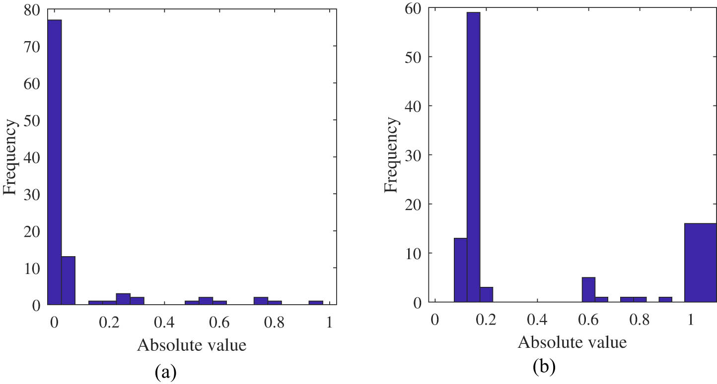
Superpixel histogram: (a) histogram for background superpixel and (b) histogram for foreground superpixel.

3.2.3 Two-dimensional feature

Although one-dimensional feature is effective, it ignores two-dimensional information. A two-dimensional measurement index called f l a t n e s s is proposed. The so-called flatness is the difference between the pixel and the surrounding pixels. The flatness of foreground superpixel is relatively low because their values differ less from those of their neighbors, as shown in Figure 4. The flatness of background superpixel is relatively high because their values differ more from those of their neighbors. Figure 4(a) is rougher than Figure 4(b). The steps for solving flatness are given in Algorithm 1.

Algorithm 1 Solving flatness
Require candidate foreground matrix of image D c .
Ensure the flatness G of the candidate foreground matrix.
1:	Convolute the image using the formula by (4) and get the horizontal gradient H .
2:	Convolute the image using the formula by (5) and get the vertical gradient V .
3:	Calculate the flatness of each pixel by (6) and get the gradient of the candidate foreground matrix G .

(4) H = 1 2 1 0 0 0 − 1 − 2 − 1 ,

(5) V = − 1 0 1 − 2 0 2 − 1 0 1 ,

(6) G = H 2 + V 2 .

Figure 4

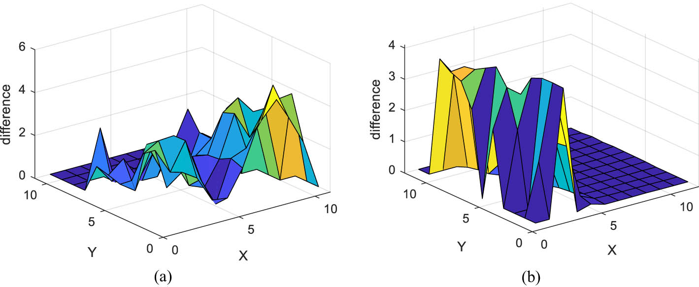
(a) Flatness for background superpixel and (b) flatness for foreground superpixel.

3.3 Background update

Existing RPCA models [10,23] are prone to voids when performing slow-moving FS. To this end, the background updating strategy of SPF-CNN is as follows: first, ten frames without foreground are selected as the background of the model. If a new frame needs to be detected, this frame and ten frames of the background are put into the IRCUR [25] model for decomposition. After detection, if the model contains foreground, the background template will not be updated. Otherwise, the oldest frame is replaced with the detecting frame.

3.4 Procedures of SPF-CNN

The steps of the proposed algorithm are shown in Figure 5. The steps for model training are given in Algorithm 2. The network structure information of 1D-CNN is given in Table 1. Padding is configured as “same,” and the stride is set to 1. The designed network contains 8 layers and 5.8k learnable in total. The batch size is 64. The model uses an Adam optimizer to iterate through 100 epochs. FLOPs (floating points of operations) of SPF-CNN is 4.5k.

Figure 5

Block diagram for proposed model.

4.1 Experimental platform

The operating system of the experimental platform is Windows 10 Professional. It is equipped with an Intel Core i9-10900K processor, 40 GB of RAM, and an RTX 3090 graphics card with 24 GB of VRAM.

4.2 Experimental dataset

CDNet2014 [28] is a widely recognized dataset for motion target detection, with manually annotated foreground information in each dataset. Additionally, the CDNet2014 official website includes test results for numerous mainstream methods. CDNet2014 actually includes more datasets, with a total of 11 categories of datasets. However, the focus of SPF-CNN is on handling dynamic backgrounds and can only process image sequences from fixed cameras. Therefore, datasets such as cameraJitter, PTZ, Turbulence, Low Framerate, and Night Videos are not used for experimentation. The reasons include camera jitter, PTZ, and turbulence having shaky cameras, Low Framerate having too few manually annotated images, and Night Videos having a disproportionately small annotated area, making them unsuitable for model training. Image sequences from the remaining six subsets with 31 image sequences are used for experiments. During the experiments, each image’s size retains the original resolution.

4.3 Experimental setting

Since the proposed method is a supervised approach, the training set must include manually annotated images with foreground information. As not every dataset’s first image contains annotated information, the initial images from each dataset that contain foreground information and annotations are used for model training. Two hundred images are selected for training based on file sequence numbers and specific conditions. Because the comparison methods contain supervised methods, in order to test the generalization ability of supervised methods at the same time, the image sequences of each category are divided into two groups, one for model training and the other for model testing. The grouping information of the video is the same as that in the literature [29], as shown in Table 2. About 200 pictures containing moving objects from each video in one category are selected from each video sequence in each group for model training. F1-score [23] is used for objective evaluation.

4.4 Evaluation index

F1-score [23] is used for objective evaluation and it is calculation methods are shown as follows:

where False Negative (FN) represents a pixel that is determined to be a negative sample but is actually a positive sample. False Positive (FP) represents a pixel that is determined to be a positive sample but is actually a negative sample. True Negative (TN) represents a pixel that is determined to be a negative sample and is indeed a negative sample. True Positive (TP) represents a pixel that is determined to be a positive sample and is indeed a positive sample.

4.5 Comparison algorithms

The comparison algorithms include the following: TW-Net [29], BSUV-Net [2], FgSegNet [18], SWCD [30], KDE [31], GMM [8], PSPNet [32], CPB [33], 3PBM [34], MOD_GAN [35], RMFF [36], and NLTFN [37]. TW-Net [29], BSUV-Net [2], and FgSegNet [18] belong to supervised algorithms and fall under the category of deep learning methods. TW-Net [29], BSUV-Net [2], and FgSegNet [18] use the same training and testing sets, as shown in Table 2. SWCD [30], KDE [31], CPB [33], 3PBM [34], RMFF [36]a NLTFN [37], and GMM [8] build their model based on background pixels, making it an unsupervised algorithm. MOD_GAN [35] is a method based on generative adversarial networks (GANs), falling under the category of unsupervised algorithms.

4.6 Results and discussion

Table 4 provides the F1-score values for comparative methods and SPF-CNN in experiments conducted on 31 videos. Because of the limited space, the category name and video name of the video are abbreviated. A higher F1-score indicates better detection performance. BSUV-Net [2] and FgSegNet [18] obtain the lowest F1-score, likely due to the difference between the training and testing scenarios, leading to insufficient model generalization. SWCD [30], RMFF [36], and NLTFN [37] better utilize spatio-temporal constraints to build the model, resulting in superior performance compared to KDE [31] and GMM [8]. From Table 4, we can see that SWCD [30] and SPF-CNN achieve the highest values for F1-score on average. SPF-CNN and SWCD achieve 16 and 11 highest F1-score in 31 videos, respectively. SWCD [30] is second only to SPF-CNN. It means that SPF-CNN is effective. From the perspective of F1-score, the effect of SPF-CNN is the best.

Figure 6 shows some visualization results. Due to the existence of floating snowflakes and lake surface, GMM [8] and KDE [31] mistakenly detect snowflakes and lake surface as foreground. This method uses superpixel segmentation to extract the features of background and foreground. Because the features of snowflakes and lake surface have been included in the background when training the model, this method does not mistakenly judge snowflakes as foreground. GMM [8] and KDE [31] produce holes when processing slow-moving objects. Because the template updating strategy of this method is based on the frame. If the current frame does not contain moving targets, the background model is updated with the current frame, so there is no hole when detecting slow motion. Table 3 gives the time consumption for each algorithm. The time in Table 3 only includes the actual test time, not the model training time. The detection time of FGSegNet [18] and BSUV-Net [2] is least because they just need simple matrix calculation when detecting. The models of KDE [31], GMM [8], and SWCD [30] are simple, thus their running speed is fast. Although TW-Net is based on deep learning, it needs matrix decomposition to obtain candidate prospects, so the time complexity is high. SPF-CNN needs superpixel segmentation and feature extraction, so the time complexity is the highest. Although SPF-CNN has a relatively high computational time, it is based on MATLAB, and there will be more optimization possibilities in the future.

Figure 6

Some examples of the detection results. From left to right: input image, ground truth, GMM [8], SPF-CNN (ours) and KDE. For each video, we pick one frame to present.

References

[1] Y.-F. Li, L. Liu, J.-X. Song, Z. Zhang, and X. Chen, “Combination of local binary pattern operator with sample consensus model for moving objects detection,” Infrared Phys. Technol., vol. 92, pp. 44–52, 2018. 10.1016/j.infrared.2018.05.009Search in Google Scholar
[2] O. Tezcan, P. Ishwar, and J. Konrad, “Bsuv-net: a fully-convolutional neural network for background subtraction of unseen videos,” In: The IEEE Winter Conference on Applications of Computer Vision, 2020, pp. 2774–2783. 10.1109/WACV45572.2020.9093464Search in Google Scholar
[3] D. Sakkos, H. Liu, J. Han, and L. Shao, “End-to-end video background subtraction with 3d convolutional neural networks,” Multimedia Tools Appl., vol. 77, no. 17, pp. 23023–23041, 2018. 10.1007/s11042-017-5460-9Search in Google Scholar
[4] J. Liao, G. Guo, Y. Yan, and H. Wang, “Multiscale cascaded scene-specific convolutional neural networks for background subtraction,” in: Pacific Rim Conference on Multimedia, Springer, 2018, pp. 524–533. 10.1007/978-3-030-00776-8_48Search in Google Scholar
[5] L. A. Lim and H. Y. Keles, “Learning multi-scale features for foreground segmentation,” Pattern Anal. Appl., vol. 23, no. 3, pp. 1369–1380, 2020. 10.1007/s10044-019-00845-9Search in Google Scholar
[6] D. Liang, Z. Wei, H. Sun, and H. Zhou, “Robust cross-scene foreground segmentation in surveillance video,” in: 2021 IEEE International Conference on Multimedia and Expo (ICME). IEEE, 2021, pp. 1–6. 10.1109/ICME51207.2021.9428086Search in Google Scholar
[7] O. Barnich and M. Van Droogenbroeck, “Vibe: A universal background subtraction algorithm for video sequences,” IEEE Trans. Image Process, vol. 20, no. 6, pp. 1709–1724, 2010. 10.1109/TIP.2010.2101613Search in Google Scholar PubMed
[8] C. Stauffer and W. E. L. Grimson, “Adaptive background mixture models for real-time tracking,” in: Proceedings. 1999 IEEE Computer Society Conference on Computer Vision and Pattern Recognition (Cat. No PR00149), vol. 2, IEEE, 1999, pp. 246–252. Search in Google Scholar
[9] M. Hofmann, P. Tiefenbacher, and G. Rigoll, “Background segmentation with feedback: The pixel-based adaptive segmenter,” In: 2012 IEEE Computer Society Conference on Computer Vision and Pattern Recognition Workshops. IEEE, 2012, pp. 38–43. 10.1109/CVPRW.2012.6238925Search in Google Scholar
[10] E. J. Candès, X. Li, Y. Ma, and J. Wright, “Robust principal component analysis?,” J. ACM, vol. 58, no. 3, pp. 1–37, 2011. 10.1145/1970392.1970395Search in Google Scholar
[11] S. E. Ebadi and E. Izquierdo, “Foreground segmentation with tree-structured sparse rpc,” IEEE Trans. Pattern Anal. Machine Intelligence, vol. 40, no. 9, pp. 2273–2280, 2018. 10.1109/TPAMI.2017.2745573Search in Google Scholar PubMed
[12] J. Wang, G. Xu, C. Li, Z. Wang, and F. Yan, “Surface defects detection using non-convex total variation regularized RPCA with kernelization,” IEEE Trans. Instrument. Measurement, vol. 70, 2021, pp. 1–13. 10.1109/TIM.2021.3056738Search in Google Scholar
[13] Y. Guo, G. Liao, J. Li, and X. Chen, “A novel moving target detection method based on RPCA for sar systems,” IEEE Trans. Geosci. Remote Sens., vol. 58, no. 9, pp. 6677–6690, 2020. 10.1109/TGRS.2020.2978496Search in Google Scholar
[14] D. Giveki, “Robust moving object detection based on fusing atanassov’s intuitionistic 3d fuzzy histon roughness index and texture features,” Int. J. Approximate Reasoning, vol. 135, pp. 1–20, 2021. 10.1016/j.ijar.2021.04.007Search in Google Scholar
[15] Y. Wang, Z. Luo, and P.-M. Jodoin, “Interactive deep learning method for segmenting moving objects,” Pattern Recognit. Lett., vol. 96, pp. 66–75, 2017. 10.1016/j.patrec.2016.09.014Search in Google Scholar
[16] M. Sultana, A. Mahmood, S. Javed, and S. K. Jung, “Unsupervised deep context prediction for background estimation and foreground segmentation,” Machine Vision Appl., vol. 30, no. 3, pp. 375–395, 2019. 10.1007/s00138-018-0993-0Search in Google Scholar
[17] M. Braham and M. Van Droogenbroeck, “Deep background subtraction with scene-specific convolutional neural networks,” in: 2016 International Conference on Systems, Signals and Image Processing (IWSSIP), IEEE, 2016, pp. 1–4. 10.1109/IWSSIP.2016.7502717Search in Google Scholar
[18] L. A. Lim and H. Y. Keles, “Foreground segmentation using convolutional neural networks for multiscale feature encoding,” Pattern Recognit. Lett., vol. 112, pp. 256–262, 2018. 10.1016/j.patrec.2018.08.002Search in Google Scholar
[19] G. Rahmon, F. Bunyak, G. Seetharaman, and K. Palaniappan, “Motion u-net: Multi-cue encoder-decoder network for motion segmentation,” in: 2020 25th International Conference on Pattern Recognition (ICPR), IEEE, 2021, pp. 8125–8132. 10.1109/ICPR48806.2021.9413211Search in Google Scholar
[20] T. Liu, “Moving object detection in dynamic environment via weighted low-rank structured sparse RPCA and Kalman filtering,” Math. Problems Eng., vol. 2022, pp. 1–11, 2022. 10.1155/2022/7087130Search in Google Scholar
[21] Ş. Işık, K. Özkan, and Ö. N. Gerek, “Cvabs: moving object segmentation with common vector approach for videos,” IET Comput. Vision, vol. 13, no. 8, pp. 719–729, 2019. 10.1049/iet-cvi.2018.5642Search in Google Scholar
[22] O. Oreifej, X. Li, and M. Shah, “Simultaneous video stabilization and moving object detection in turbulence,” IEEE Trans. Pattern Anal. Machine Intelligence, vol. 35, no. 2, pp. 450–462, 2012. 10.1109/TPAMI.2012.97Search in Google Scholar PubMed
[23] Y. Li, G. Liu, Q. Liu, Y. Sun, and S. Chen, “Moving object detection via segmentation and saliency constrained RPCA,” Neurocomputing, vol. 323, pp. 352–362, 2019. 10.1016/j.neucom.2018.10.012Search in Google Scholar
[24] S. Javed, A. Mahmood, S. Al-Maadeed, T. Bouwmans, and S. K. Jung, “Moving object detection in complex scene using spatiotemporal structured-sparse RPCA,” IEEE Trans. Image Processing, vol. 28, no. 2, pp. 1007–1022, 2019. 10.1109/TIP.2018.2874289Search in Google Scholar PubMed
[25] H. Cai, K. Hamm, L. Huang, J. Li, and T. Wang, “Rapid robust principal component analysis: Cur accelerated inexact low rank estimation,” IEEE Signal Processing Letters, vol. 28, pp. 116–120, 2020. 10.1109/LSP.2020.3044130Search in Google Scholar
[26] J. Zhao, R. Bo, Q. Hou, M.-M. Cheng, and P. Rosin, “Flic: Fast linear iterative clustering with active search,” Comput. Visual Media, vol. 4, no. 4, 333–348, 2018. 10.1007/s41095-018-0123-ySearch in Google Scholar
[27] P. Sulewski, “Equal-bin-width histogram versus equal-bin-count histogram,” J. Appl. Stat., vol. 48, no. 12, pp. 2092–2111, 2021. 10.1080/02664763.2020.1784853Search in Google Scholar PubMed PubMed Central
[28] Y. Wang, P.-M. Jodoin, F. Porikli, J. Konrad, Y. Benezeth, and P. Ishwar, “Cdnet 2014: An expanded change detection benchmark dataset,” In 2014 IEEE Conference on Computer Vision and Pattern Recognition Workshops, pp. 393–400, 2014. 10.1109/CVPRW.2014.126Search in Google Scholar
[29] Y. Li, “Moving object detection for unseen videos via truncated weighted robust principal component analysis and salience convolution neural network,” Multimedia Tools Appl., vol. 81, pp. 1–12, 2022. 10.1007/s11042-022-12832-0Search in Google Scholar
[30] S. Isik, K. Özkan, S. Günal, and Ö. N. Gerek, “Swcd: a sliding window and self-regulated learning-based background updating method for change detection in videos,” J. Electronic Imaging, vol. 27, no. 2, p. 023002, 2018. 10.1117/1.JEI.27.2.023002Search in Google Scholar
[31] A. Elgammal, D. Harwood, and L. Davis, “Non-parametric model for background subtraction,” in: European Conference on Computer Vision, Springer, Berlin, Heidelberg, 2000, pp. 751–767. 10.1007/3-540-45053-X_48Search in Google Scholar
[32] D. Liang, B. Kang, X. Liu, P. Gao, X. Tan, and S. Kaneko, “Cross-scene foreground segmentation with supervised and unsupervised model communication,” Pattern Recognition, vol. 117, p. 107995, 2021. 10.1016/j.patcog.2021.107995Search in Google Scholar
[33] W. Zhou, S. Kaneko, M. Hashimoto, Y. Satoh, and D. Liang, “Foreground detection based on co-occurrence background model with hypothesis on degradation modification in dynamic scenes,” Signal Processing, vol. 160, pp. 66–79, 2019. 10.1016/j.sigpro.2019.02.021Search in Google Scholar
[34] S. M. Roy and A. Ghosh, “Foreground segmentation using adaptive 3 phase background model,” IEEE Trans. Intelligent Transport. Syst., vol. 21, no. 6, pp. 2287–2296, 2019. 10.1109/TITS.2019.2915568Search in Google Scholar
[35] M. Sultana, A. Mahmood, S. Javed, and S. K. Jung, “Unsupervised moving object detection in complex scenes using adversarial regularizations,” IEEE Trans. Multimedia, vol. 23, 2020, pp. 2005–2018. 10.1109/TMM.2020.3006419Search in Google Scholar
[36] Q. Qi, X. Yu, P. Lei, W. He, G. Zhang, J. Wu, and B. Tu, “Background subtraction via regional multi-feature-frequency model in complex scenes,” Soft Computing, vol. 27, no. 20, pp. 15305–15318, 2023. 10.1007/s00500-023-07955-xSearch in Google Scholar
[37] Y. Yang, Z. Yang, and J. Li, “Novel RPCA with nonconvex logarithm and truncated fraction norms for moving object detection,” Digit. Signal Process, vol. 133, 103892, 2023. 10.1016/j.dsp.2022.103892Search in Google Scholar
[38] C. Stauffer and W. E. L. Grimson, “Adaptive background mixture models for real-time tracking,” in: Proceedings. 1999 IEEE Computer Ssociety Conference on Computer Vision and Pattern Recognition (Cat. No PR00149), vol. 2, IEEE, 1999, pp. 246–252. Search in Google Scholar
© 2024 the author(s), published by De Gruyter
This work is licensed under the Creative Commons Attribution 4.0 International License.
Articles in the same Issue
- Regular Articles
- AFOD: Two-stage object detection based on anchor-free remote sensing photos
- A Bi-GRU-DSA-based social network rumor detection approach
- Task offloading in mobile edge computing using cost-based discounted optimal stopping
- Communication network security situation analysis based on time series data mining technology
- The establishment of a performance evaluation model using education informatization to evaluate teacher morality construction in colleges and universities
- The construction of sports tourism projects under the strategy of national fitness by wireless sensor network
- Resilient edge predictive analytics by enhancing local models
- The implementation of a proposed deep-learning algorithm to classify music genres