Resilient edge predictive analytics by enhancing local models

1.1 Emergence of edge computing (EC)

The advancement in communication technologies has paved the way for significant progress in artificial intelligence (AI). This surge is primarily due to the colossal volume of data generated by mobile and Internet of Things (IoT) devices that can now be effectively transmitted and accumulated. One major offshoot of these developments is EC. EC is a novel computing paradigm that shifts the computation closer to the source of data generation, right at the network’s edge, near sensors and end users. This approach ensures optimal use of resources and enables services that require real-time decision-making, delay-sensitive responses, and are context-aware [1].

1.2 Synergy between AI and EC

As AI solutions often require substantial data processing capabilities and appreciate minimal latency for real-time services, the integration of AI and EC is emerging swiftly. This amalgamation can primarily be categorized into two segments: “AI for edge,” which aspires to enhance EC using AI techniques, and “AI on edge,” which perceives EC as a utility for the efficient deployment of AI systems [2]. A plethora of “AI on Edge” applications have already shown success, offering a wide range of predictive services such as anomaly detection, regression, classification, and clustering. Notably, by harnessing “AI on Edge,” considerable costs associated with data transmission to the Cloud can be saved [3].

The union of AI and EC has indeed heralded a new era of technology. By pushing AI capabilities to the edge, we are not only decentralizing intelligence but also ensuring that decision-making is faster, more efficient, and less reliant on distant data centers. However, as with all nascent integrations, some challenges need to be addressed, especially when delving deeper into predictive analytics within the EC framework.

1.3 Predictive analytics in EC environments: Challenges and limitations

Predictive analytics, relying heavily on machine learning (ML) models, have found significant applications in domains such as smart cities and sustainable agriculture. In smart cities, technology is leveraged to enhance city services and the overall quality of life for its inhabitants, with tasks such as traffic predictions, energy consumption estimations, and aiding transportation companies in anticipating potential route issues. In sustainable agriculture, ML models are invaluable during both the pre-production (predicting crop yields, and soil property assessments) and production phases (disease and weed detection, and soil nutrient management). These ML models transition from raw data processing to advanced tasks like regression and classification [4].

However, when applied in the EC context, several challenges emerge. Conventional ML systems designed for “AI on Edge” applications typically have each edge node (or node for short) accessing its local data and containing ML models trained solely with these data. Despite nodes potentially operating under similar conditions and gathering data from like environments, the unique statistical characteristics of their data render their models noninterchangeable. In realistic EC scenarios, where nodes might fail due to connectivity issues or security breaches, the current system design means that functioning nodes cannot readily take over the predictive tasks of their failing counterparts [5].

1.4 A novel approach to enhance reliability in EC

The challenges highlighted necessitate the presence of “surrogate nodes” or “substitute nodes” that can efficiently process requests from failing nodes. The current paradigm of localized training (training each node’s models with only its local data) does not cater to this need. Furthermore, the idea of having a centralized backup, such as a Cloud server, is untenable in EC due to the sheer volume of internode data transfers, which contradicts the principles of EC.

Our proposed solution targets the heart of this issue: we aim to enhance the adaptability of models on neighboring nodes. The goal is to enable these nodes to efficiently handle “unfamiliar” data from failing nodes. This is achieved by actively sharing and integrating statistical signature information during the training process. However, the realization of this vision presents its own set of challenges:

1. Determining the best surrogate node(s) when a node failure arises.

2. Formulating context-aware strategies for nodes to extract and share relevant data signatures from potential failure-prone counterparts.

3. Ascertain the type and amount of data that should be shared to ensure the surrogate nodes perform on par with the original nodes.

To address these intricacies, we offer a comprehensive framework. This design integrates strategies to extract and combine data statistics from peer nodes, creating resilient models that maintain predictive performance even during node failures. Through rigorous testing using varied real-world datasets in diverse distributed computing scenarios, our framework showcases its capability to preserve and, in some instances, surpass the performance levels of systems without node failures, outshining traditional centralized approaches.

1.5 Limitations of traditional approaches in EC contexts

Historically, numerous strategies have been employed to tackle the challenges posed by node failures. Some of the pioneering efforts [6,7] adopted a straightforward approach: replications and backups. The primary philosophy behind this was to maintain duplicate versions or replicas of the nodes. In this setup, systems would operate under the assumption that the principal node remains functional. In the event of the main node’s failure, the replicas would step in to ensure continuity. However, such a strategy is resource-intensive. Creating and preserving these replicas demands a significantly higher allocation of bandwidth, storage, and computational resources, making it a less favorable solution in EC contexts.

Another well-established method to circumvent node failures is through the process of checkpointing [8,9, 10,11]. In this approach, systems periodically generate and save snapshots (termed as checkpoints) of the nodes’ states. When a node encounters a failure, the system can resort to the most recent snapshot to restore the node to its last operational state. While conceptually sound, this method comes with its own set of drawbacks. It can be taxing in terms of storage and bandwidth usage, particularly when these snapshots are stored centrally. Furthermore, certain types of node failures, such as those arising from power outages or network disruptions, that render a node entirely inaccessible cannot be remedied simply by restoring a previous state. In such scenarios, an entirely new node would be needed to replace the failed one, utilizing the saved snapshot.

Contrastingly, the framework we introduce in this article proposes a novel perspective on the problem. Our approach is rooted in the idea of developing generalized models on nodes, equipping them with the capability to assist their neighboring nodes during instances of failure. This method stands out by offering a unique solution that does not heavily lean on resource consumption, and instead, focuses on enhancing the inherent capacities of the nodes.

The article is organized as follows: Section 2 reports on the related work and our technical contribution; Section 3 formulates our problem; Section 4.1 introduces the rationale of our framework; Section 5 reports on the experimental setup, performance evaluation, and comparative assessment; Section 6 discusses the results and remaining problems; and Section 7 concludes the article.

4.1 Global sampling (GS) strategy

GS is based on a random sampling node N j ’s dataset, i.e., Γ ( D j ) ⊂ D j . N i receives samples from neighbors’ datasets and expands the local dataset as D ¯ i = D i ∪ { Γ ( D j ) } , ∀ j , j ≠ i . The size of the sample ∣ Γ ( D j ) ∣ and sample mixing rate α = ∣ Γ ( D j ) ∣ ∣ D j ∣ ∈ ( 0 , 1 ) is controlled by N i , which affects the generalizability of enhanced model f ˜ i S .

4.2 Guided sampling strategies

GS gives a relatively average summary of D j , making it ideal for datasets distributed evenly, i.e., it does equally count all the samples. However, sampled data can convey a variety of characteristics; thus, feeding the enhanced models with such data without taking into account that these characteristics cannot boost the generalizability of the enhanced models. To allow control of the sampling process of { D j } , we introduce guided sampling strategies that exploit data clustering to selectively capture data that will be included during the training of the enhanced models. We rely on vector quantization (clustering) of D j ∀ j in light of exploiting the information derived by the corresponding clusters (representatives). Such representatives, a.k.a., centroids w j k , k = 1 , … , K , partition D j into K disjoint subsets D j ≡ ⋃ k = 1 K { D j k } with ⋂ k = 1 K D j k = ∅ . The way such centroids are used yields certain variants.

4.3 Strategies based on information adjacency

The strategies we have introduced so far treat all the N i ’s neighboring nodes N j ∈ N i equally in terms of influence and statistical importance. Note, we take training samples and/or statistics according to the strategies from all the communicating neighboring nodes’ datasets D j . However, we could expect that such a method cannot scale given a large number of neighboring nodes. Moreover, if the underlying data distributions of some of the D j datasets we sample from differ significantly from D i (of node N i ), we anticipate that these samples possibly impact the performance of the enhanced model f ˜ i s negatively. Especially when there is no significant statistical correlation between D i and D j , like spatio-temporal correlations or overlapping probability densities, the derived enhanced model f ˜ i s loses its generalization capacity while yielding a simply averaging model with insufficient predictive capability. The statistical dependencies of the data either derived from spatio-temporal correlations (e.g., nodes spatially close together can sense similar contextual information) or closeness/overlapping of density functions motivated us to selectively engage only those neighboring nodes N j whose sampled data/statistics could positively contribute to the training and predictive performance of the f ˜ i s .

Grouping together the nodes with similarly distributed data seems to be a sensible option, as by only letting the models have controlled access to less “unfamiliar” data within the group, we expect them to be less affected by instances that are more likely to be in nodes from foreign groups that will damage their performance. However, the effect of grouping is heavily affected by the adopted grouping method. Hence, the improper grouping may even negatively impact the models’ predictability. We then investigate how grouping helps under different circumstances and compare the possible gain in performance instead of turning to grouping strategies completely. In this context, we introduce strategy variants based on this information adjacency that leverage inherent or latent information embedded within the nodes’ data to achieve grouping for each of the strategies above. These adjacency variants function exactly the same as their counterparts except that, when generating the enhanced training data D ¯ i , only the D j datasets from a pre-determined nodes adjacency list N j ∈ A i ⊂ N i are considered, i.e.,

Since grouping strategies value the similarities of the nodes’ data (statistical distances) more than the physical distance (though sometimes they are closely related), we revoked the 1-hop restriction on them. Nodes in the same group are not necessarily reachable to each other within 1 time of data exchange. The topology of the grouping is demonstrated in Figure 3. The nodes adjacency list A i is determined according to strategies mentioned above tailored to the characteristic of the nodes’ data. Hence, for each strategy, its adjacency variant defines the corresponding list A i as follows.

Figure 3

Two (groupings) adjacency lists of nodes A i and A k for node N i and node N k , respectively, determined according to data characteristics and dependencies.

4.4 Model-driven data (MD) strategy

The MD strategy is proposed as a different one from the above data-driven strategies, where nodes do not need to disseminate real data among them. The rationale of MD is that node N i generates training data points indirectly from its neighboring nodes’ local models f j , N j ∈ N i . Specifically, the MD strategy is not heavily dependent on the scale of D j ; instead, the training samples Γ ( D j ) are locally generated at N i , once N j has sent only its local model parameters f j along with certain statistics of the input domain X j to N i . Then, N i can use f j and the corresponding statistics of X j to locally fabricate the training samples ( x ˆ , y ˆ ) ∈ Γ ( D j ) according to the distribution of D j captured by the local model f j . That is, N j calculates the input mean vector μ j and input standard deviation σ j from X j and the unbiased regression variance estimate σ ˆ j 2 = 1 ∣ D j ∣ − d − 1 ∑ k = 1 ∣ D j ∣ ( y k − f j ( x k ) ) 2 on the output Y of the local model f j . These statistics along with the model f j are sent to node N i , which can locally generate training pairs ( x ˆ , y ˆ ) such that y ˆ = f j ( x ˆ ) + ε j , where the error ε j is a Gaussian random variable with expectation zero and variance σ ˆ j 2 . The fabricated input x ˆ in node N i is randomly sampled from N ( μ j , σ j 2 ) . Node N i generates then a sample of α ∣ D j ∣ fabricated pairs instances ( x ˆ , y ˆ ) from each received model f j such that

In short, the fabricated input, x ˆ , is drawn from a Gaussian distribution characterized by mean μ j and variance σ j 2 . The fabricated output, y ˆ , is then computed by applying the model f j to the input x ˆ and adding Gaussian noise ε j with zero mean and variance σ ˆ j 2 .

The adjacency model-driven (AMD) strategy depends on the distances of the mean vector μ i and σ i over node N i ’s dataset with the fabricated mean vector μ j and σ j sent over from node N j , i.e.,

A node N j is considered adjacent to node N i if the Euclidean distance between their mean vectors is less than or equal to a threshold θ , and the absolute difference between their standard deviations is also within this threshold.

5.1 Datasets

The GNFUV [30] dataset was collected during the experiments of our project GNFUV5.1 ^[1]. The dataset contains readings of temperature and humidity from sensors mounted on four unmanned surface vehicles (USVs) monitoring the sea surface in a coastal area in Athens, Greece. The local data D i , i = 1 , … , n = 4 , recorded by the USVs exhibit different distribution while bearing some spatiotemporal correlation. With it, we simulated a distributed system (referred to directly as GNFUV in the remainder of the article) of four nodes, with each of the nodes corresponding to a USV. We used “temperature” as the input variable x ∈ R to predict the output variable “humidity” y ∈ R . The Accelerometer [31] dataset contains three independent variables that correspond to fixed interval readings of accelerometers that are attached to a fan on x , y , and z axes. This dataset is used in regression tasks as the accelerometer readings are used to predict the percentage of the fan’s speed. A weight was attached to the fan with three different setups to affect the readings in different ways. We expect readings from the same setup to be distributed more similar to each other than those from other setups. Hence, we split the original data into three parts w.r.t. their weights and assigned each part to each node obtaining n = 3 nodes in total.

The last dataset is the Combined Cycle Power Plant (CCPP) [32], which contains four types of environmental sensor readings like temperature and pressure. With these readings, the power plant’s total output power is predicted. We proceeded with clustering these data using Gaussian Mixture Model (GMM) into several clusters. UMAP[33] was also used to reduce the clustering results to three dimensions for viewing them intuitively, as shown in Figure 4). Therefore, the clustered data were assigned to n = 3 nodes associated with the best GMM setting.

Figure 4

The visualization of the best clustering results we got on CCPP dataset (3 clusters).

5.2 Experimental scenarios

With the GNFUV, Accelerometer and CCPP datasets, we obtain three scenarios: (i) a distributed computing system that has spatiotemporally correlated data across its nodes (hereinafter referred to as GNFUV scenario), (ii) a distributed computing system that has natural data split across its nodes, but the correlation between nodes’ data is relatively weaker (hereinafter referred to as Accelerometer scenario), and (iii) a distributed computing system that has randomly split data across its nodes (hereinafter referred to as CCPP scenario).

GNFUV dataset was collected when the USVs were moving along their parallel routes (as shown in Figure 5). By being spatially close, USVs were moving along adjacent routes and thus were more likely to collect spatiotemporally correlated contextual data. Hence, the nodes that have their data collected by USVs from directly adjacent routes are considered to be adjacent forming their adjacency lists { A } , e.g., USV 3’s list A 3 = { USV 1 , USV 2 } (Figure 5).

Figure 5

The trajectories of the USVs building GNFUV dataset.

For both the accelerometer and CCPP datasets, as there are three nodes for these two scenarios, we found that each node has only one adjacent node in their lists { A } ; we also experimentally found that, e.g., if N 1 is considered to be adjacent to both N 2 and N 3 , we obtained the same results as those obtained without considering the adjacency lists { A } . This outcome was derived from applying the criteria in the strategies based on information adjacency taking into account the distributions of the nodes’ data.

Specifically, for the CCPP dataset, as shown in Figure 4, there are patterns of separation of different nodes’ data, thus forming almost separable clusters. In addition, for the Accelerometer dataset, as shown in Figure 6, all three nodes’ data are centered around the origin 3D point ( 0 , 0 , 0 ) having a significant amount of overlapping. Note that, as shown in Figure 6, the three nodes’ data can be roughly seen as distributed in three spheres that share the same center; their standard deviations are directly proportional to the spheres’ radii. Hence, the nodes having their data distributed in similar spaces (i.e., closer standard deviation) could be put into the same group, as we found by applying the criteria in the adjacency strategies (detailed later).

Figure 6

The distribution of different all nodes’ Accelerometer data in (right) 3D plane; (left) 2D plane over the two principal components using UMAP.

For predictive models, we adopt the supervised learning support vector regression (SVR) model y = f i ( x ; b i ) , b i ∈ X ⊂ R d over nodes in our experiments. Note, other ML models could be also adopted, which do not spoil the evaluation methodology.

5.3 Model performance assessment

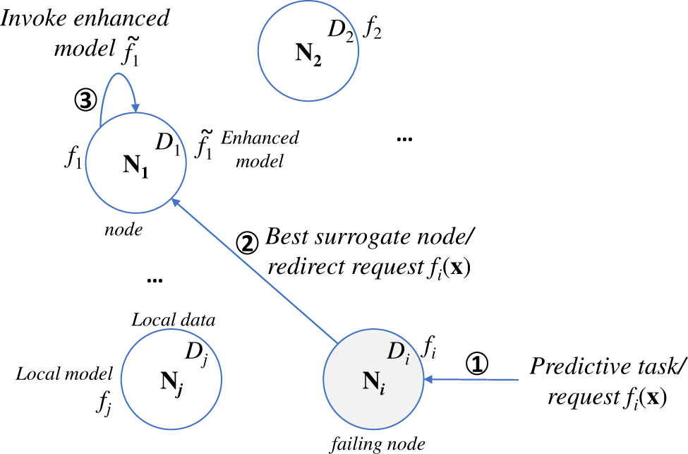
Upon nodes (e.g., USVs) failure, our framework seeks the most appropriate surrogate node N i and strategy s ∈ { GS, NCG, CG, WG } given a mixing rate α to train the enhanced models on the surrogate node. We devised a systematic approach to assess the performance of the enhanced models trained with different parameters for each node adopting grid search for tuning. For each node N i and strategy, we set mixing rates α ∈ { 0.02 , … , 0.2 } . The corresponding datasets D ¯ i , s are built based on D i and the n − 1 Γ ( { D j } ) derived from { D j } for each strategy s . Then, we trained the enhanced SVR models f ˜ i s for each D ¯ i , s and evaluated the models’ performance in terms of the root mean square error (RMSE) between actual output y and model prediction y ˆ .

For each node N i , the data we evaluated the models on include the enhanced data D ¯ i and the raw data D j from the neighboring nodes N j ∈ N i . We obtain an insight into the influences brought by applying our approach to the node’s capabilities to handle its own data and data from others. The evaluation was conducted using 10-fold cross-validation, and the data included in { D j } are excluded from the models’ evaluation on D j data. Moreover, to compare and contrast the influence brought by our approach, we evaluated the performance of (i) the (Global) Cloud model, i.e., the model that was trained on all the nodes’ data ( D G ) transferred from nodes to Cloud (denoted by f G ), which serves as the baseline model, and (ii) the local models, i.e., models trained only on local data D i (denoted by f i ) on the same kind of data they were trained with. For the GNFUV dataset, we obtained f G ( D G ) (the baseline) and four local models f i ( D i ) , i = 1 , … , 4 . Note that a similar setting was repeated for the CCPP and Accelerometer datasets. We expect prediction error for some f ˜ i s ( D j ) to fall above f G ( D G ) and for some to fall below f G ( D G ) . Prediction error below or close to that of f G ( D G ) is desired as it indicates that the parameters corresponding to these models provide more accurate predictions than the Cloud. Furthermore, the accuracy of f ˜ i s ( D j ) is expected to be less than f i ( D i ) as local models have ideal performance on local data.

Figure 7 shows the results of the enhanced model f ˜ 3 s of node N 3 ; similar results are obtained for the rest nodes over the GNFUV dataset. Figure 7 shows the performance (RMSE) of local, Cloud, and enhanced models against different mix-rate values across all strategies. One could observe that N 3 is not a good candidate as a substitute node for N 1 and N 4 because the errors of f ˜ 3 s ( D 1 ) and f ˜ 3 s ( D 4 ) are above the baseline f G ( D G ) . However, as evidenced, N 3 is an appropriate substitute for node N 2 if N 2 fails. As with NCG and CG, for certain α values, the corresponding enhanced model f ˜ 3 of N 3 outperformed the baseline on D 2 (accuracy is higher than that of f G ( D G ) ). This indicates that given our strategies, when N 2 fails, N 3 can take over N 2 ’s predictive tasks without needing to transfer to N 2 ’s data to Cloud (for building a new model therein). More importantly, substitute N 3 gives better predictions than the Cloud. This denotes the resilience capacity of the system adopting our strategies.

Figure 7

GNFUV: Sensitivity analysis of the α (mix rate) on the performance evaluation of the local model f 3 ( D 3 ) , Cloud model f G ( D G ) and the enhanced models f ¯ 3 s ( D i ) in N 3 under the four strategies (GS,NCG,CG,WG).

5.4 Deployment of our scenarios

5.4.1 Decision-making and assignment resilience policy

We have first identified the best strategy s and mix-rate α for every pair of potentially failing node N i and potentially substitute node N j . Then, in a distributed computing system with n nodes, we obtain adequate information to guide the invocation of substitute nodes in the case of node failures.

We introduce a directed graph G ( V , ℰ ) to guide the node invocation and visualize the guidance as illustrated in Figure 8 for the GNFUV scenario. The vertices V represent edge nodes; we introduce one extra vertex referring to Cloud ( G ). A directed edge e i j ε , s ∈ ℰ starts from node N i and ends with N j attached with a RMSE value ε and strategy s ∈ S (the mixing rate α was omitted for clearance). The semantics of e i j ε , s is that if a predictive task request is received to failing node N j , then a potential substitute node N i could, at its best, provide a RMSE ε from its enhanced model f ˜ i s given the best selected strategy s . For instance, the edge e 42 in Figure 8 indicates that upon N 2 ’s failure, the best substitute node N 4 can invoke its enhanced model f ˜ 4 G S given the best strategy GS obtaining RMSE 2.13. The edges e 12 and e 32 indicate that N 1 and N 3 can serve N 2 ’s requests when it fails both with NCG as best strategy obtaining RMSE of 7.98 and 3.95, respectively. Thus, the second-best substitute for N 2 is N 3 offering the second-lowest RMSE. If the best substitute N 4 is unreachable (or, e.g., overloaded), then N 3 can be reached next and so on. If none of the candidate substitutes is reachable, then the request goes to Cloud G as a last resort. A recursive edge e i i ε , s indicates the RMSE achieved by N i ’s enhanced model over its own data D i with best strategy s . The graph is disseminated to all nodes for localized decision-making. In our experiments, we investigate the system’s performance when the best substitute is available to serve the directed requests from the failing nodes.

Figure 8

GNFUV: Directed graph G ( V , ℰ ) guiding the decision-making for the most appropriate substitute node and strategy upon node failures.

With the directed graph, the system is fully operable in EC environments where node failures happen. To further better understand the benefits brought by our approach, we evaluated the system’s performance with full, half, and no guidance at all with node failing probability p from 0% to 100%. To avoid the chain reaction of the surrogate nodes failing one after another and allowing clearer insight into the system’s behaviour, we assume that when a node fails, its substitute node(s) will work. Specifically, at every predictive task request to a node N i , we draw with probability p its status. If N i is not failed, then the node processes the request locally using its local model. Otherwise, i.e., N i fails/unavailable, then, we consider the following node assignment resilience policies:

1. Random substitute assignment: The request is assigned to a randomly chosen nonfailing node, which locally processes the task using its local model. This is a baseline policy to investigate what happens without the graph guidance of our approach and without invoking the enhanced models on substitute nodes (zero guidance).

2. Random substitute assignment with best enhanced model: The request is assigned to a randomly chosen nonfailing node, which locally processes the task using its best enhanced model given the provided graph (half guidance).

3. Guided substitute assignment: The request is assigned to the most appropriate substitute node as per graph, which locally processes the task using its best enhanced model as per graph (full guidance).

Remark 2

In Figure 8, none of the edges is associated with WG. Compared to other strategies, WG did not achieve a single best on arbitrary pairs of failing N i and substitute N j . WG is designed for special anomalous datasets yielding suboptimal performance. Our test results using the local outlier factor (LOF) algorithm do conform with that, as the resulting anomaly rate is 7.6%, which is normal for LOF.

5.4.2 Predictive accuracy assessment

The prediction accuracy results of the aforementioned resilience policies are shown in Figure 9 against node failure probability p for the GNFUV dataset. We compare the results obtained from these assignment policies including: (i) the cloud-based assignment policy, i.e., sending the predictive tasks to the cloud (which maintains a global model trained over all nodes’ data, i.e., f G ( D G ) ) and (ii) the average nonfailing nodes assignment policy, where we obtain the average prediction by invoking the best enhanced models (with the best selected strategy) over the expanded datasets of all nonfailing nodes, i.e.,

(15) f ˜ 0 = 1 n − 1 ∑ i = 1 n − 1 f ˜ i s ( D ¯ i ) .

Figure 9

GNFUV: System performance against node failure probability p across different node assignment resilience policies.

One could observe that the system’s predictability with the guided substitute assignment always out performs the Cloud-based policy even when p reaches 100%. This indicates that our approach helps the system to maintain better performance than the Cloud even when a node is unavailable all the time.

Moreover, when p < 20 % , the system performance is quite close to the best local enhanced models. This denotes that our resilience method supports the system to maintain performance equivalent to the cases of no failures at all, especially when p is at a relatively low level. This further proves its potency in improving the system’s resilience in EC environments. Furthermore, the performance of the random substitute assignment with the best enhanced model (half guidance) helps to keep the system predictability capacity at relatively higher levels than that of the baseline until p reached around 50%. That is, even if nodes fail half of the time, exploiting the enhanced models of the nonfailing nodes provides better predictability than directing the requests to the Cloud. In addition, by comparing the half guidance with the random substitute assignment (zero guidance), the former was able to reduce the RMSE by half. This evidences that our resilience approach endows the system with a fair amount of flexibility: even if we do not direct the predictive task requests to the best substitute node due to reasons like load balance all the time, it can still contribute to boosting the system’s predictability performance via using the enhanced models from randomly chosen substitute nodes. Evidently, the full guidance policy exploits the full information in graph G , and thus, resilience is achieved without needing requests to be directed to Cloud even if with high node failure probabilities.

5.4.3 Load impact

We investigated the impact of the substitute assignment policies on the number of invocations on each node, i.e., extra load. Figure 10 shows that with the full guidance policy, node extra loads are relatively balanced. Although we expect node imbalance given tasks workloads; requests to failing node N i are directed to the same best substitute N j . If multiple nodes have the same best substitute node N j , upon their failures, all the requests will be directed to N j , thus, causing imbalanced loads. In systems that are susceptible to node imbalance, this could be alleviated, e.g., by directing a percentage β % of requests to the best substitute node and directing the rest ( 1 − β ) % to the second-best substitute node. Evidently, the challenge to find the optimal β to achieve load balance and system performance is on our future research agenda.

Figure 10

GNFUV: Extra load per node in the system with full guidance assignment policy and half/zero guidance policy.

5.5 Incorporating the adjacency strategies

From the results in Section 5.3, we obtained insights into the framework’s feasibility and potential based on the first four global strategies (global strategies refer to s ∈ S G = { GS, NCG, CG, WG, MD } , we only consider first four data-driven strategies GS, NCG, CG and WG). To further assess the applicability of our framework in distributed ML systems, we incorporate model-driven strategy MD and adjacency strategies ( s ∈ S A = { AGS, ANCG, ACG, AWG, AMD } ) to the decision-making graphs and assignment resilience policies, thus, obtaining a holistic framework evaluated across our scenarios.

5.5.1 Predictive accuracy

The evaluation process, settings, and metrics remain the same as the experiments in Section 5.3. Figures 11, 12 and 13 show the sensitivity analysis regarding the predictive performance across global and adjacency strategies against ratio α on each representative node for all three scenarios. While in general for each node, the trends of every strategy are almost similar, we did observe different behaviours in the strategies’ performances in different scenarios. This indicates that different strategies yield different performance behaviours depending on the scenario settings and, evidently, on the underlying data. We aimed at investigating this variety obtaining the optimal decision-making graphs per scenario.

Figure 11

Accelerometer: Sensitivity analysis of the α (mix rate) on the performance evaluation of the local model f 1 ( D 1 ) , Cloud model f G ( D G ) and the enhanced models f ¯ 1 s ( D i ) in N 1 under global and adjacency strategies.

Figure 12

CCPP: Sensitivity analysis of the α (mix rate) on the performance evaluation of the local model f 1 ( D 1 ) , Cloud model f G ( D G ) and the enhanced models f ¯ 1 s ( D i ) in N 1 under global and adjacency strategies.

Figure 13

GNFUV: Sensitivity analysis of the α (mix rate) on the performance evaluation of the local model f 2 ( D 2 ) , Cloud model f G ( D G ) and the enhanced models f ¯ 2 s ( D i ) in N 2 under global and adjacency strategies.

For node N 1 over the Accelerometer dataset/setting (Figure 11), the overall trend shows that the performance of the enhanced models of N 1 is not affected significantly by the ratio α for most of the strategies. As all the errors represented by the green lines (corresponding to Node N 3 ’s data) are relatively higher than the baseline model ( f G ( D G ) ), it indicates that node N 1 is not considered an effective surrogate node for helping node N 3 . Instead, it works quite effectively in serving requests from node N 2 , as many of the orange lines (GS, AGS, WG, AWG, and MD) corresponding to N 2 ’s data are far below the baseline and even the local model’s error ( f 1 ( D 1 ) ). Furthermore, in MD strategy, as the blue line indicates, the enhanced model’s performance ( f ¯ 1 ( D ¯ 1 ) ) is even better than the local model ( f 1 ( D 1 ) ). It means the added information from other nodes helped the node to perform better on its local data. We obtain similar results and conclusions for the rest of the nodes in the Accelerometer scenario.

In CCPP scenario, node N 1 (shown in Figure 12) favors the representative information from other neighboring nodes. As the green and orange lines show (corresponding to nodes N 3 ’s and N 2 ’s data), for all the strategies, with the increase of statistical information (i.e., larger α ), the enhanced models almost always perform better on the data of nodes N 2 and N 3 . Moreover, the stable blue lines indicate that in this process, the enhanced models’ performance on local data is hardly negatively affected. Similar to Accelerometer, the MD strategy is the best-performing strategy, reaching fairly low errors for all three nodes’ data. Similar results and conclusions have been obtained for the rest of the nodes in this scenario.

The performances of the enhanced models of GNFUV’s node N 2 are more complicated. As shown in Figure 13, node N 2 could help by being the surrogate node for node N 4 effectively well adopting the strategies GS, NCG, CG, WG, and MD (indicated by red lines). As for node N 3 , it could only help by adopting the adjacency variants AGS, ANCG, ACG, and AWG (indicated by green lines). When it comes to node N 1 , no strategy could help effectively (indicated by orange lines). Thus, in the cases where N 1 fails, turning to N 3 or N 4 instead of N 2 might be advisable (depending on the evaluation results on them). These behaviors of the enhanced models are evidence of the unique value brought by the adjacency variants as sometimes feasible results on some nodes could only be attained with them. The introduction of them did help to excavate more possibilities with the guidance of natural or statistical clues of adjacency.

5.5.2 Improved decision-making and assignment resilience policies

For each scenario, we provide the optimal directed graphs G ( V , ℰ ) , as shown in Figure 14. For the GNFUV scenario, compared to the results we obtained from the first four global strategies (GS, NCG, CG, and WG), for all the available global and adjacency strategies (ten in total), we are able to improve nearly half of the decisions reflected by the edges, i.e., 44% of the edges in the directed graph have now lower RMSE values. Moreover, six out of seven improvements were achieved by s ∈ S A , which highlighted the importance of leveraging the adjacency information mechanisms for building the enhanced models over the nodes belonging to the same group.

Figure 14

Directed graphs G ( V , ℰ ) guiding the decision-making for the most appropriate substitute node and strategy upon node failures for all scenarios adopting the global and adjacency strategies.

For Accelerometer and CCPP, s ∈ S A were able to achieve one best result compared to s ∈ S G . The adjacency of the nodes in these scenarios was obtained through the correlation between adjacent clusters and their corresponding statistical signatures. Furthermore, it is worth mentioning that CCPP favors the model-driven strategy MD significantly so that seven out of nine of its best results (according to decision making) were achieved by adopting MD. This is expected as the nodes in the CCPP scenario were grouped given the GMM clustering. It is also evidence of our framework’s ability to capture the characteristics of the dataset and respond with the most proper solution. We observed similar conclusions when we conducted experiments over Accelerometer as we forced the testing data to contain as many outliers as possible with the outlier scores generated by LOF. It turned out that the strategies WG and AWG (tailored to be targeting anomalous datasets) obtain half of the best results. This further proves the applicability of our framework across unfamiliar nodes’ datasets. In the Accelerometer scenario, we obtained five out of nine best results with the GS and its adjacency variant AGS, indicating that the information of it is evenly distributed within the whole dataset. Considering how the Accelerometer dataset was collected, as discussed before, this conclusion lay within our expectations.

As for the holistic performance of the framework against possible node failures shown in Figure 15, there are several latent but important things worth mentioning. The starting point of all three lines (hereinafter referred to as starting point) in each subplot represents the average error of the system when no node failure occurs. f ˜ 0 represents the influence brought by the enhanced models. That is, how the system would perform as a whole when it only relies on enhanced models to operate. The relative positions of the starting point, f ˜ 0 , and the baseline f G ( D G ) could give us insights into the system’s performance and the suitability of adopting enhanced models. In detail, the results from the GNFUV scenario show similar trends to the results we obtained from the experiments in Section 5.4.1. Overall, s ∈ S A obtain better predictive performance against failure probability compared to s ∈ S G . Moreover, the guided substitute assignment over the adjacency strategies obtains always better results than the centralized approach even with a high failure probability. This indicates the robustness and fault tolerance of the proposed framework by adopting the concept of enhanced models and the information adjacency for node grouping. As the starting point is located between f ˜ 0 and f G ( D G ) , it indicates that GNFUV is well suited for the proposed framework. Because lower f ˜ 0 and higher f G ( D G ) means the system favors separately built enhanced models instead of a centralized global model. Furthermore, guided substitute assignment helped to maintain the system’s performance better than the baseline even when p reached 100%. In the Accelerometer scenario, the global model seems to outperform all the other models. This was expected due to the strong correlation among the spherical data clusters, however, at the expense of the centralized data transfer and lack of distributed learning. More interestingly, one can observe in Figure 15 (Accelerometer) that the f ˜ 0 obtains almost the same predictive performance as that with the guided substitute assignment with a failure probability of 50%. This indicates the capability of our framework to recommend effectively the best possible strategies even if the nodes fail at every time instance with a probability of 0.5. In the CCPP scenario, f ˜ 0 is very close to the starting point, indicating its affinity to enhanced models. Also, no matter what strategy we adopt, a node could be easily supported by another (the red line is very close to the green line), which means that we can adopt any optimal strategy obtaining similar performance with the baseline/centralized approach. As a result, at node failure probability of 100%, CCPP’s performance could be maintained better than the baseline and even close to the starting point.

Figure 15

Framework fault-tolerant predictive performance against node failure probability p across different node assignment resilience policies (global and adjacency strategies) for all the scenarios.

5.5.3 Load impact

We can observe some load imbalance in all scenarios in Figure 16 when we also incorporate the adjacency strategies. As mentioned before, this problem could be alleviated by not always using the best substitute node with some trade-offs of performance, which is left in our future research agenda.

Figure 16

Extra load per node in the system with full guidance assignment policy and half/zero guidance policy for all the scenarios adopting global and adjacency strategies.

6.1 Impact of information adjacency strategies

The discrepancy in the gain from introducing information adjacency, as shown in the experimental results for different scenarios, highlights that the effectiveness of nodes' grouping through this method is heavily dependent on the efficiency of the process for acquiring the lists { A i } , ∀ N i . While the adjacency strategies in the scenarios over Accelerometer and CCPP datasets obtained similar results to the global (non-adjacency) strategies, the adjacency strategies in the GNFUV scenario yield solid improvements. Furthermore, of all the best results shown in Figure 14 that are obtained with strategies s ∈ S A , 87.5% of them correspond to AGS and AMD, which coincide with our speculation of AGS and AMD being able to benefit more from the derived lists { A } in Section 4.3. The limited number of nodes also affects this phenomenon and expect ANCG, ACG, and AWG to show their potential in scenarios with a relatively larger number of nodes.

It is worth mentioning that, though strategies s ∈ S A are able to achieve the best results, as shown in Figure 14, 67% of them are recursive (shown by the blue edges ( e i , i )). This means strategies s ∈ S A are especially efficient at maintaining the enhanced models’ performance on its local data ( D i ). We examined the experimental results and found that the enhanced models corresponding to these recursive edges did perform satisfactorily well as surrogate models that operate on other nodes’ data while being able to offer almost similar performance on local data D i as compared to the local models ( f i ). This denotes that it is possible to only equip each of the nodes with one enhanced model that could handle all kinds of predictive service requests (both local requests and requests from failing nodes) with a minor sacrifice of predictive performance.

6.2 Model maintenance

One of the most important functionalities our framework could provide is effective model maintenance. As in dynamically changing distributed ML systems, the ML models should not remain static because of certain changes in the underlying data (like concept drifts). Instead, such systems should have the ability to keep up with the data changes by recognizing new patterns introduced by concept drifts in, e.g., data streams and retraining them with instances that follow these patterns. We expect that the proposed graph-based guidance (i.e., the directed graphs) to hold for the most part as it is built by excavating inter-nodes’ data relationships. When the system detects meaningful drifts in a node’s data, novel instances should be efficiently sent to whichever nodes have enhanced models that require data from the changing node for model maintenance. In the current stage, our framework focuses on guidance building in the case of node failures and only considers the best substitute node and strategy. In fact, facilitated by the flexibility of the framework, through intelligently grouping nodes and allocating enhanced models invocation, it is possible to make a node failure tolerant system that only requires each of the nodes to maintain one or two models with slight performance trade-offs as compared to a system that operates on an “all best” strategy (i.e., follow the directed graph strictly) when node failure occurs. Such a system is well suited for model maintenance as the process only requires the transferring of a few novel instances and the retaining of several models. The investigation of this mechanism is included in our future research agenda.

References

[1] J. Ren, Y. Pan, A. Goscinski, and R. A. Beyah, “Edge computing for the internet of things,” IEEE Netw., vol. 32, no. 1. pp. 6–7, 2018. 10.1109/MNET.2018.8270624Search in Google Scholar
[2] S. Deng, H. Zhao, W. Fang, J. Yin, S. Dustdar, and A. Y. Zomaya, “Edge intelligence: The confluence of edge computing and artificial intelligence,” IEEE Internet Things J., vol. 7, no. 8. pp. 7457–7469, 2020. 10.1109/JIOT.2020.2984887Search in Google Scholar
[3] W. Shi, J. Cao, Q. Zhang, Y. Li, and L. Xu, “Edge computing: Vision and challenges,”. IEEE Internet Things J., vol. 3, no. 5. pp. 637–646, 2016. 10.1109/JIOT.2016.2579198Search in Google Scholar
[4] M. A. Jan, et al. “An AI-enabled lightweight data fusion and load optimization approach for internet of things,” Future Gener. Comput. Syst., vol. 122, pp. 40–51, 2021. 10.1016/j.future.2021.03.020Search in Google Scholar PubMed PubMed Central
[5] J. Wang, S. Pambudi, W. Wang, and M. Song, “Resilience of iot systems against edge-induced cascade-of-failures: A networking perspective,” IEEE Internet Things J., vol. 6, no. 4. pp. 6952–6963, 2019b. 10.1109/JIOT.2019.2913140Search in Google Scholar
[6] A. Borg, J. Baumbach, and S. Glazer, “A message system supporting fault tolerance,” ACM SIGOPS Operating Systems Review, vol. 17, no. 5. pp. 90–99, 1983. 10.1145/773379.806617Search in Google Scholar
[7] B. Cully, G. Lefebvre, D. Meyer, M. Feeley, N. Hutchinson, and A. Warfield, “Remus: High availability via asynchronous virtual machine replication,” In Proceedings of the 5th USENIX symposium on networked systems design and implementation, pp. 161–174. San Francisco, 2008. Search in Google Scholar
[8] J. Sherry, P. X. Gao, S. Basu, A. Panda, A. Krishnamurthy, C. Maciocco, et al. “Rollback-recovery for middleboxes,” In Proceedings of the 2015 ACM Conference on Special Interest Group on Data Communication, pp. 227–240, 2015. 10.1145/2785956.2787501Search in Google Scholar
[9] M. Mudassar, Y. Zhai, and L. Lejian, “Adaptive fault-tolerant strategy for latency-aware IoT application executing in edge computing environment,” IEEE Internet Things J., vol. 9, no. 15. pp. 13250–13262, 2022. 10.1109/JIOT.2022.3144026Search in Google Scholar
[10] M. Siavvas, and E. Gelenbe, “Optimum interval for application-level checkpoints,” In 2019 6th IEEE International Conference on Cyber Security and Cloud Computing (CSCloud)/2019 5th IEEE International Conference on Edge Computing and Scalable Cloud (EdgeCom), pp. 145–150, 2019. 10.1109/CSCloud/EdgeCom.2019.000-4Search in Google Scholar
[11] Y. Harchol, A. Mushtaq, V. Fang, J. McCauley, A. Panda, and S. Shenker, “Making edge-computing resilient,” In Proceedings of the 11th ACM Symposium on Cloud Computing, SoCC ’20, pp. 253–266, New York, NY, USA. Association for Computing Machinery, 2020. 10.1145/3419111.3421278Search in Google Scholar
[12] J. P. Sterbenz, D. Hutchison, E. K. Çetinkaya, A. Jabber, J. P. Rohrer, M. Schller, et al., “Resilience and survivability in communication networks: Strategies, principles, and survey of disciplines,” Comput. Netw., vol. 54, no. 8. pp. 1245–1265, 2010. Resilient and Survivable networks.10.1016/j.comnet.2010.03.005Search in Google Scholar
[13] K. A. Delic, “On resilience of IoT systems: The internet of things (ubiquity symposium),” Ubiquity, 2016 February:1–7. 10.1145/2822885Search in Google Scholar
[14] J. Beutel, K. Römer, M. Ringwald, and M. Woehrle, “Deployment Techniques for Sensor Networks,” pp. 219–248, 2009. 10.1007/978-3-642-01341-6_9Search in Google Scholar
[15] M. M. H. Khan, H. K. Le, M. LeMay, P. Moinzadeh, L. Wang, Y. Yang, et al., “Diagnostic power tracing for sensor node failure analysis,” In Proceedings of the 9th ACM/IEEE international conference on information processing in sensor networks, pp. 117–128, 2010. 10.1145/1791212.1791227Search in Google Scholar
[16] S. Shao, X. Huang, H. E. Stanley, and S. Havlin, “Percolation of localized attack on complex networks,” New J. Phys., vol. 17, no. 2. p. 023049, 2015. 10.1088/1367-2630/17/2/023049Search in Google Scholar
[17] S. N. Shirazi, A. Gouglidis, A. Farshad, and D. Hutchison, “The extended cloud: Review and analysis of mobile edge computing and fog from a security and resilience perspective,” IEEE J. Sel. Areas Commun., vol. 35, no. 11. pp. 2586–2595, 2017. 10.1109/JSAC.2017.2760478Search in Google Scholar
[18] S. Kounev, P. Reinecke, F. Brosig, J. T. Bradley, K. Joshi, V. Babka, et al., “Providing Dependability and Resilience in the Cloud: Challenges and Opportunities,” pp. 65–81. Springer Berlin Heidelberg, Berlin, Heidelberg, 2012. 10.1007/978-3-642-29032-9_4Search in Google Scholar
[19] A. Shafahi, M. Najibi, Z. Xu, J. Dickerson, L. S. Davis, and T. Goldstein, “Universal adversarial training,” AAAI Conference on Artificial Intelligence, vol. 34, no. 04. pp. 5636–5643, 2020. 10.1609/aaai.v34i04.6017Search in Google Scholar
[20] E. Wong, L. Rice, and J. Z. Kolter, “Fast is better than free: Revisiting adversarial training,” CoRR, abs/2001. vol. 03994, 2020. Search in Google Scholar
[21] T. Bai, J. Luo, J. Zhao, B. Wen, and Q. Wang, “Recent advances in adversarial training for adversarial robustness,” CoRR, vol. abs/2102.01356, 2021. 10.24963/ijcai.2021/591Search in Google Scholar
[22] H. Daumé III, “Frustratingly easy domain adaptation,” arXiv:http://arXiv.org/abs/arXiv:0907.1815, 2009. Search in Google Scholar
[23] A. Farahani, S. Voghoei, K. Rasheed, and A. R. Arabnia, “A brief review of domain adaptation,” Advances in Data Science and Information Engineering, pp. 877–894, 2021. 10.1007/978-3-030-71704-9_65Search in Google Scholar
[24] A. Samanta, F. Esposito, and T. G. Nguyen, “Fault-tolerant mechanism for edge-based iot networks with demand uncertainty,” IEEE Internet Things J., vol. 8, no. 23. pp. 16963–16971, 2021. 10.1109/JIOT.2021.3075681Search in Google Scholar
[25] D. Takao, K. Sugiura, and Y. Ishikawa, Approximate fault-tolerant data stream aggregation for edge computing,” In Big-Data-Analytics in Astronomy, Science, and Engineering: 9th International Conference on Big Data Analytics, BDA 2021, Virtual Event, December 7–9, 2021, Proceedings, Berlin, Heidelberg, Springer-Verlag, pp. 233–244, 2021. 10.1007/978-3-030-96600-3_17Search in Google Scholar
[26] C. Wang, C. Gill, and C. Lu, “Frame: Fault tolerant and real-time messaging for edge computing,” In 2019 IEEE 39th International Conference on Distributed Computing Systems (ICDCS), pp. 976– 985. IEEE, 2019a. 10.1109/ICDCS.2019.00101Search in Google Scholar
[27] Q. Wang, J. M. Fornes, C. Anagnostopoulos, and K. Kolomvatsos, “Predictive model resilience in edge computing,” Accepted on IEEE 8th World Forum on Internet of Things 2022. 10.1109/WF-IoT54382.2022.10152282Search in Google Scholar
[28] C. Chatfield, “Model uncertainty, data mining and statistical inference,” Journal of the Royal Statistical Society. Series A (Statistics in Society), vol. 158, no. 3. pp. 419–466, 1995. 10.2307/2983440Search in Google Scholar
[29] A. E. Raftery, D. Madigan, and J. A. Hoeting, “Bayesian model averaging for linear regression models,” J. Am. Stat. Assoc., vol. 92, no. 437. pp. 179–191, 1997. 10.1080/01621459.1997.10473615Search in Google Scholar
[30] N. Harth, and C. Anagnostopoulos, “Edge-centric efficient regression analytics,” In 2018 IEEE EDGE, pp. 93–100. IEEE, 2018. 10.1109/EDGE.2018.00020Search in Google Scholar
[31] G. S. Sampaio, A. R. de Aguiar Vallim Filho, L. S. da Silva, and L. A. da Silva, “Prediction of motor failure time using an artificial neural network,” Sensors, vol. 19, no. 19. p. 4342, 2019. 10.3390/s19194342Search in Google Scholar PubMed PubMed Central
[32] P. Tüfekci, “Prediction of full load electrical power output of a base load operated combined cycle power plant using machine learning methods,” Int J. Electr. Power Energy Syst., vol. 60, pp. 126–140, 2014. 10.1016/j.ijepes.2014.02.027Search in Google Scholar
[33] L. McInnes, J. Healy, and J. Melville, “UMAP: Uniform manifold approximation and projection for dimension reduction,” 2018. 10.21105/joss.00861Search in Google Scholar
Received: 2023-08-04
Revised: 2023-10-23
Accepted: 2024-01-22
Published Online: 2024-05-13
© 2024 the author(s), published by De Gruyter
This work is licensed under the Creative Commons Attribution 4.0 International License.
Articles in the same Issue
1. Regular Articles
2. AFOD: Two-stage object detection based on anchor-free remote sensing photos
3. A Bi-GRU-DSA-based social network rumor detection approach
4. Task offloading in mobile edge computing using cost-based discounted optimal stopping
5. Communication network security situation analysis based on time series data mining technology
6. The establishment of a performance evaluation model using education informatization to evaluate teacher morality construction in colleges and universities
7. The construction of sports tourism projects under the strategy of national fitness by wireless sensor network