Laminar Rayleigh–Benard convection in a closed square field with meshless radial basis function method
-
Irfan Santosa
 ,
Syamsul Hadi
,
Syamsul Hadi

Abstract
Research on natural convection is exciting in some experimental and numerical cases, especially in rectangular cavities with relatively low heat dissipation and thermal control systems with low cost, reliability, and ease of use. The present study will use the meshless radial basis function method to solve the velocity formulation of the Navier–Stokes equations by varying some nominal Rayleigh numbers of 104, 105, and 106. The numerical accuracy is compared with the previous research. The advantages of the meshless method are that it does not require a structured mesh and does not require inter-nodal connectivity. The results show that the temperature pattern is identical to the previous research. The calculations have been done for three different Rayleigh numbers of 104, 105, and 106 for 151 × 151 nodes. The variations of the Ra number will affect the isothermal, velocity contours, and Nusselt number.
Nomenclature
-
-
gravitational acceleration (m/s2)
-
-
height and length of the enclosure (m)
-
-
Nusselt number (–)
- Pr
-
Prandtl number (–)
- Ra
-
Rayleigh number (–)
-
-
dimensionless temperature of the cold wall (–)
-
-
dimensionless temperature of the hot wall (–)
-
-
dimensionless horizontal and vertical velocity (–)
-
-
coordinates axis
-
-
thermal diffusivity (m2/s)
-
-
coefficient of thermal expansion (1/K)
-
-
pressure
-
-
dimensionless temperature (–)
-
-
kinematic viscosity (m2/s)
1 Introduction
Convection is heat transfer between a hot/cold surface and a liquid, which is a complex physical phenomenon [1]. Among the different types of convection, natural convection in a rectangular cavity is of great interest to researchers because of the transport process in fluids where the motion arises from the relationship between density differences and gravity, which is very common in engineering and environmental problems. This analysis is widely applied to build (i.e., ventilation) airflow patterns in greenhouses, solar energy systems, and solar air heaters and to cool electronic equipment, desalination systems, and devices that use convection to perform DNA amplification by polymerase chain reaction , which has a great deal of scientific importance. Therefore, it is interesting to study natural convection in several experimental and numerical cases, where thermal dissipation is relatively low and the thermal control system is of low-cost, reliable, and easy to use. Research on natural convection numerically in a rectangular cavity with a liquid above the vertical heating plate was conducted by Rahman et al. [2] and the effect of natural convection on metal solidification was investigated by Suprianto et al. [3], Muthuvel et al. [4] conducted numerical research by varying the type of mesh (hexahedral, tetrahedral, and polyhedral) in a rectangular cavity flow. The effect of thermal field boundaries on natural convection in rectangular cavity planes was investigated by Basak et al. [5], where the boundary layer formation was examined. It has also been observed that the thermal boundary layer develops in more than 80% of voids for uniform heating. In contrast, the thermal boundary layer forms in about 60% of voids for non-uniform heating when the value of Ra = 103.
Most natural convection research on square cavities is currently classified into two groups. The first is differential heating of a heated square enclosure; the effects of thermal boundary conditions at the left and right walls were investigated by Ben Cheikh et al. [6], the effects of a two-dimensional domain with vertical walls heated differently were observed by Costa et al. [7], and analysis of the shape of a cube with heated vertical walls was performed by Accary and Raspo [8]. The second is a cover that is heated from below and cooled from above (Rayleigh–Benard convection [RBC]); some experimental and numerical studies on a rectangular box heated from below were performed by Calcagni et al. [9], analyzing the thermography at the lower and upper limits is the RBC observed by Platten et al. [10], and a study of natural convection in a locally heated rectangular cavity from below with a constant flux source was performed in the study of Ben Cheikh et al. [11]. The effect of wall thickness on natural convection and entropy in a cavity filled with the Al2O3–water nanofluid and heated from below was also investigated by Ishak et al. [12]. The result is that heat transfer increases with increasing heat thickness at the bottom. RBC is one of the simplest convection stabilities [13] witnessed when the homogeneous isotropic fluid is confined in a vertical direction under the influence of gravity and the upper plate is maintained at a uniform and stable temperature, lower than the lower plate that has a higher temperature. Thus, RBC is a thermo-fluid flow affected by buoyancy due to a temperature gradient first described by Rayleigh in 1916 [14]. RBC motion is also affected by the temperature difference (∆T) between the hot reservoir and the cold reservoir [15], where an increase in temperature (∆T) causes an increase in the velocity of the water molecules still, the size of the convection radius decreases.
Research on numerical simulations of natural convection and temperature distribution in supercritical fluid water in a heated sidewall cavity was conducted by Li et al. [16], where the supercritical water fluid exhibits a thinner boundary layer at much higher velocities and eventually forms a double eddies natural convection pattern in the cavity. Another numerical study is on the two-dimensional domain associated with natural convection in a rectangular cavity heated from below and cooled from above under unsteady conditions with 0.71 Pr. The Rayleigh number (Ra) in the range from 103 to Ra 106 was investigated by Ouertatani et al. [17]. The finite volume method (FVM) was used, where the momentum and energy equations were discretized using the red and black successive over relaxation method. Then, Osman et al. [18] also investigated a two-dimensional steady-state simulation of natural laminar convection in a rectangular cavity with horizontal walls heated differently with the lower wall at a higher temperature with Ra values of 103–105, and Pr values of 0.1–100 by using the FVM. The pressure and velocity terms in the momentum equations are calculated by the SIMPLE method.
Simulation studies on an L-shaped cavity heated by varying the Rayleigh number from 103 to 108 were performed by Gawas and Patil [19]. This article analyzes RBC fluid flow under steady or unsteady conditions by changing the average Nusselt number (Nu) along the wall heat line. This study concludes that the higher the Ra, the more unstable the flow structure and the effect on the Nu number. The variations of Ra values from 102 to 106 in a rectangular cavity were also studied by Syamsuri et al. [20] using the FVM. They concluded that the smaller the Ra value in the rectangular cavity, the more vertical the isothermal line phenomenon will appear, and if the Ra value is greater, the isothermal line phenomenon will be horizontal.
The present study proposes a meshless radial basis function (RBF) method to solve the Rayleigh–Benard convection. The Rayleigh–Benard convection problem is developed by the Navier–Stokes and energy equations. The pressure–velocity coupling in the momentum equations is solved by the pressure correction method. The advantages of the meshless method are that it does not require a structured mesh, is suitable for use in structured and complex domains, and does not require inter-nodal connectivity. The numerical accuracy obtained by the present study was compared with those of Ouertatani et al. [17] and Osman et al. [18]. The RBF approach is used to estimate the unknown field, and the boundaries of each sub-domain are explained. RBF does not require a part of the domain boundary to solve numerical problems, and RBF can solve problems at each node and its spatial derivatives [21]. This feature of RBF is advantageous in solving the velocity vorticity formulation of the Navier–Stokes equation because velocity gradient calculations are used to calculate the vortices determined as boundary conditions for the vorticity transport equation [22].
2 Numerical method
A high-order accurate, flexible in terms of geometry, computationally efficient, and simple-to-use numerical approach is appropriate for partial differential equation (PDE) problems. Commonly used methods usually fulfill one or two of the criteria, but not all. A fairly new approach to solving PDEs is through RBFs [23].
2.1 RBF method
The RBF has been widely applied in various numerical schemes. RBF is a natural generalization function from univariate spline polynomials to multivariate arrangements. Its main advantages are high dimensions and meshless interpolations. RBF is a function whose value depends on the distance from the central point. RBF can be easily implemented for reconstructing planes or surfaces using scattered data in 2D, 3D, or higher-dimensional domains. The RBF method is not only used in the fields of computational fluid dynamics, but also in structural analysis, and optimization. Rippa [24] proposed an algorithm for selecting a good value of the shape parameter c for multiquadric, inverse multiquadric, and Gaussian functions with RBF methods, which can significantly affect the quality of the interpolation of scattered data. The results of numerical experiments involving two-dimensional data sets showed that the algorithm consistently produced good values for the parameter c, leading to accurate and smooth interpolants with low error. The RBF method determines which produces the best mesh and is the most efficient at C 2 [25]. Best accuracy and robustness and the highest efficiency were obtained with C 2 continuous RBF which is very suitable for flow calculations around NACA-0012 airfoils. The RBF method has been applied to the general higher-order equivalent single layer (GHESL) formulation and the Differential geometry (DG) tool for the free vibrations of doubly curved laminated composite shells and panels [26]. Results show the RBF method coupled with the GHESL formulation and the DG tool provides a powerful tool for analyzing the free vibrations of complex structures, such as those found in aerospace and mechanical engineering applications. Research was made to modify the radial distances of existing RBFs for the buckling analysis of functionallly gradient materials (FGMs) rectangular plates. The results of several numerical examples showed that the modified RBF-based methods were accurate and well suited for analyzing rectangular plates made of FGM [27]. In another study, Nguyen et al. [28] presented a modified mesh-free radial point interpolation method (RPIM) to explore the nonlinear bending behavior. The results from the detailed parametric studies showed that the modified mesh-free RPIM can effectively predict the nonlinear bending behavior of FGM plates. The volume fraction, plate length-to-thickness ratio, boundary condition, and initial deflection were found to have significant effects on the bending behavior. Research on the influence of different GPL distribution patterns, GPL weight fraction, shape, and size of cut-outs on the free vibration and buckling behavior of the multilayer FG-GPLRC perforated plates with meshfree RPIM based on a higher-order shear deformation theory (HSDT) was performed by Reza et al. [29]. The results can be used to guide the development of new perforated plate structures with enhanced vibration and buckling resistance. RBF-DQ (RBF-differential quadrature) is a variant of the RBF method that it applied to the approach to the free vibration problem of laminated composite plates of arbitrary shape. The approach is shown to be effective in reducing the number of grid points per element compared to other classical approaches, while maintaining high accuracy. The results show that the appropriate RBF-DQ approach can accurately predict the natural frequencies of laminated composite plates of arbitrary shape [30].
The most widely used RBF are listed in Table 1.
Various types of RBFs [31]
| RBF | Name abbreviation |
|
Stability |
|---|---|---|---|
| Multi quadric | MQ |
|
Infinitely stable |
| Inverse multi-quadric | IMQ |
|
Infinitely stable |
| Inverse quadric | IQ |
|
Infinitely stable |
| Generalized multi-quadric | GMQ |
|
Infinitely stable |
| Gaussian | GA |
|
Infinitely stable |
| Thin page spline | TPS |
|
Stable finite |
| Linear | LN |
|
Stable finite |
| Cube | CU |
|
Stable finite |
| Single sentence | SS |
|
Stable finite |
In the RBF method, the approach to the function f is defined as follows [32]:
where
The first and second derivatives of the basis function can be determined from
where x, y are spatial vectors, r is the distance matrix,
2.2 Problem description
This article uses the two-dimensional RBF meshless model to simulate the RBC-type thermo-fluid flow. The main assumptions in this study are as follows: (a) fluids are considered incompressible (Pr 0.71) so that the effect of pressure on density variations can be neglected; (b) shear viscosity, coefficient of thermal expansion, and thermal diffusivity are kept constant; (c) temperature as a passive scalar is affected by the velocity field which is affected by buoyancy; and (d) variables are intrinsically related taking into account the effects of density differences and buoyancy forces and neglecting the viscous heat of compression dissipation work due to pressure. The domain having a height (H) = 1 and length (L) = 1 are the dimensions of the rectangular cavity plane with 151 × 151 uniform nodes. The boundary condition (Table 2) of the rectangular cavity consists of a non-slip wall u = v = 0 on all four walls. The thermal boundary conditions on the left and right walls are adiabatic, and the thermal boundary conditions on the lower and upper walls are shown in Figure 1.
Boundary conditions
| Air | ||
|---|---|---|
| Bottom wall |
|
u = v = 0 |
| Top wall |
|
u = v = 0 |
| Left wall |
|
u = v = 0 |
| Right wall |
|
u = v = 0 |

Computational domain and boundary condition (a) and (151 × 151) uniform nodes distribution (b) for a rectangular cavity.
Dimensionless parameters such as Prandtl number (Pr) and Rayleigh number (Ra) are defined as follows:
The average heat flux is determined by:
The procedure to calculate the Rayleigh–Benard problem in the current study is illustrated in Figure 2.

Research flow.
2.3 Governing equation
The Navier–Stokes equation and the energy equation are used to set up non-dimensional equations to solve the problem of thermal incompressible convection [33].
Continuity equation:
(9)Momentum equation – x directional:
(10)Momentum equation – y directional:
(11)Energy equation:
The aforementioned equations are obtained by dividing the dimensionless variable by the reference variable as follows:
The implicit Euler method is used to discretize the time derivative, and the RBF method is used to discretize the space derivative. The first step is to modify the momentum equation with the pressure term removed so that the equation becomes
Velocity component
Then, the pressure term is calculated by the equation:
Next, the actual velocity components
The energy equation is solved to get
3 Discretization
The x momentum equation can be discretized using a linear combination of RBFs, which can be expressed in the following form:
The y momentum equation can be discretized using a linear combination of RBFs, which can be expressed in the following form:
The pressure equation can be discretized as follows:
The velocity correction equation can be discretized as follows:
The discretized form for the energy equation using a linear combination of RBFs is given as follows:
where ∆t denotes the time step, superscript
4 Results and discussion
All results presented in this section are for Pr = 0.71. Computations for three different Rayleigh numbers, Ra = 104, 105, and 106, can be solved on 151 × 151 uniform nodes. Ouertatani et al. [17] used a non-uniform 2562 grid selected for computations, which had a different amount of nodes. Directional movement isothermal lines associated with Ra = 104, 105, and 106 are presented in Figures 3–5. When the Rayleigh number (Ra) is small, heat is conducted primarily through the fluid layer, and the system is in a stable conduction state. When the Ra exceeds a certain threshold value, the thermal conductive state becomes unstable and thermal convection occurs in the fluid layer. When the Rayleigh number (Ra) is increased even further beyond the threshold value for the onset of convection, the convective flow can exhibit oscillatory behavior. For Ra = 104, the flow is symmetrical and parallel to the horizontal wall, which indicates the dominant conduction heat transfer mode. As the Ra value increases, the two secondary eddies observed at the left and right angles are also symmetrical isothermal and indicate the beginning of the convection motion for Ra > 105. The isothermal contour is indeed more distorted for Ra > 105, and the higher the value of Ra, the more convection effect can be seen. The isothermal becomes curved with the strengthening of convective transport in the cavity.
![Figure 3
Isothermal contour at Ra 104: (a) present study with nodal 151 × 151, (b) [17], (c) [18].](/document/doi/10.1515/cls-2022-0204/asset/graphic/j_cls-2022-0204_fig_003.jpg)
![Figure 4
Isothermal contour at Ra 105: (a) present study with nodal 151 × 151, (b) [17], (c) [18].](/document/doi/10.1515/cls-2022-0204/asset/graphic/j_cls-2022-0204_fig_004.jpg)
![Figure 5
Isothermal contour at Ra 106: (a) present study with nodal 151 × 151, (b) [17].](/document/doi/10.1515/cls-2022-0204/asset/graphic/j_cls-2022-0204_fig_005.jpg)
Isothermal contour at Ra 106: (a) present study with nodal 151 × 151, (b) [17].
The velocity vectors of each cavity at various Ra values are shown in Figure 6, with the length of the arrows proportional to the magnitude of the velocity and the direction indicating the direction of fluid movement. For Ra = 104, it forms a vortex in the form of a circle in the middle, then the greater the value of Ra = 105 forms a vortex in the form of a circle that is getting bigger, and two vortexes are formed. While the value of Ra = 106, the vortex groove will be smoother and tighter, and two vortexes are included at the upper left and lower right ends, which are getting bigger. Once again, the clockwise movement observed agrees with the temperature profiles, providing further confirmation of the accuracy of the simulations.
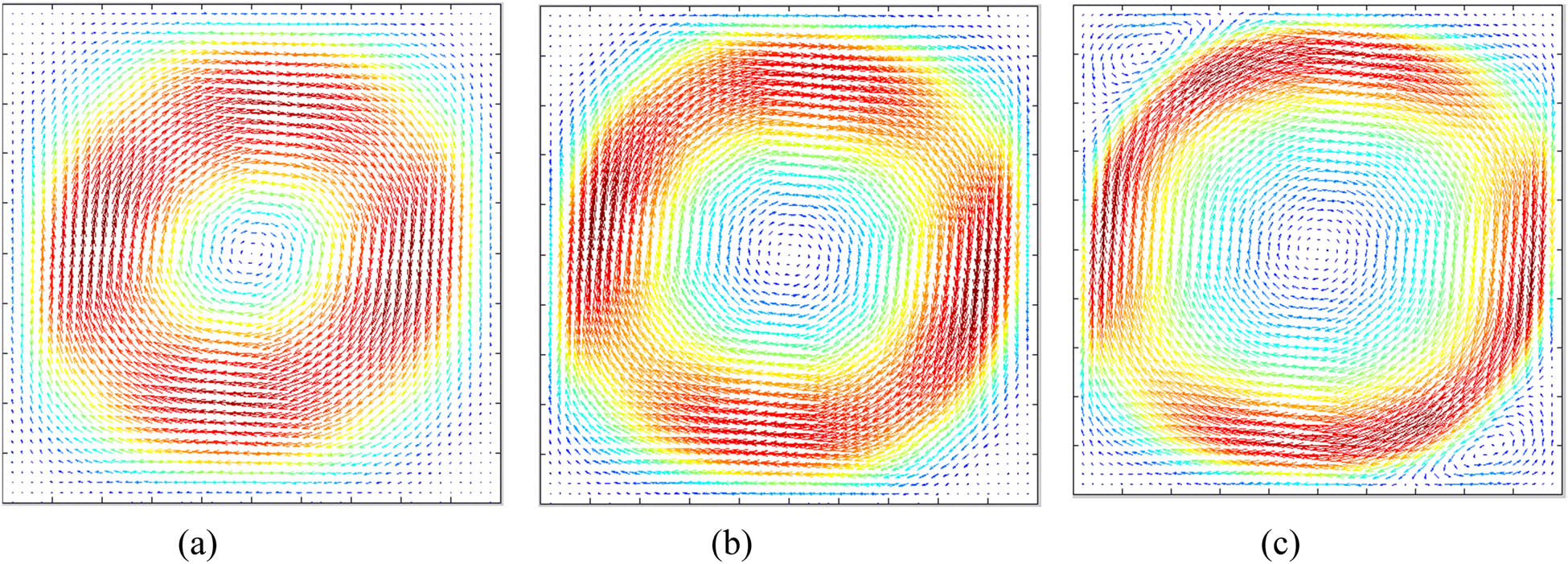
Velocity vector at (a) Ra 104, (b) Ra 105, (c) Ra 106.
Figure 7 shows fluid motion (u and v) distributed along L(x) and H(y), which is increasingly non-linear with increasing Ra value. Graph velocity u in the direction of y at the value of Ra = 104; the same velocity pattern is formed with the previous study where the highest u values are at a speed of 0.23. At the value of Ra = 105, the same pattern is created with the previous study with the highest u values at a speed of 0.33. Regarding Ra = 106, graphs show the same pattern as the earlier study; the highest u values are at a speed of 0.34.

Graph of horizontal velocity u(y) and vertical v(x) at Ra = 104, Ra = 105, Ra = 106.
The position of the y(
Comparison of the coordinate position
| Ra | [17] | Present study | ||
|---|---|---|---|---|
|
y(
|
x(
|
y(
|
x(
|
|
| 104 | 0.8023 | 0.8263 | 0.8122 | 0.8323 |
| 105 | 0.8636 | 0.8973 | 0.8735 | 0.9061 |
| 106 | 0.9036 | 0.9359 | 0.9135 | 0.9355 |
Table 4 compares the average Nusselt number obtained from the current numerical simulations for Ra = 104,105, and 106 at Pr = 0.71 for incompressible fluids with the previous literature results. It is evident from Table 4 that the current results are based on the previous numerical results.
5 Conclusion
In this study, the Rayleigh–Benard natural convection in a rectangular cavity has been analyzed numerically. Using the meshless RBF method, the effect of the Ra of 104, 105, and 106 on thermal, streamline, and velocity distribution of fluid movement in the cavity has been investigated in detail. The results show that on the isothermal contour, the higher the Ra value, the convection effect can be seen clearly, and the isotherm becomes curved with the strengthening of convective transport in the cavity. Likewise, the higher the Ra value, the smoother and tighter the vortex grooves on the streamlined contour, and a circle pattern is formed in the middle and gets bigger. Then the Nusselt number also increases with increasing Ra value. This meshless RBF method can solve Rayleigh–Benard natural convection, and the results are in good agreement with those from the previous study.
Acknowledgments
The authors thank Universitas Sebelas Maret for the financial support through Hibah Non APBN UNS 2022.
-
Funding information: This research was supported by the Universitas Sebelas Maret (Grant No. 254/UN27.22/HK.01.03/2022).
-
Author contributions: The authors made authors made substantial contributions to the conception and design of the study. The authors took responsibility for conceptualization, methodology, investigation. Writing – original draft, formal analysis (I. S., E. P. B), supervision (S.H., A. T. W.); all authors have read and agreed to the published version of the manuscript.
-
Conflict of interest: Authors state no conflict of interest.
References
[1] du Puits R. Time-resolved measurements of the local wall heat flux in turbulent Rayleigh–Bénard convection. Int J Heat Mass Transf. 2022;188:122649. 10.1016/j.ijheatmasstransfer.2022.122649.Search in Google Scholar
[2] Rahman MM, Mamun MAH, Billah MM, Rahman S. Natural convection flow in a square cavity with internal heat generation and a flush mounted heater on a side wall. J Nav Archit Mar Eng. 2011;7(2):37–50. 10.3329/jname.v7i2.3292.Search in Google Scholar
[3] Suprianto H, Budiana EP, Widodo PJ. Natural convection differential method numeric simulation on metal. Mekanika. 2017;16(September):53–9. 10.20961/mekanika.v16i2.35057.Search in Google Scholar
[4] Muthuvel GJA, Prakash N, Manikan C. Numerical simulation of flow inside. Int J Tech Res Appl. 2014;2(3):87–94. www.ijtra.com.Search in Google Scholar
[5] Basak T, Roy S, Balakrishnan AR. Effects of thermal boundary conditions on natural convection flows within a square cavity. Int J Heat Mass Transf. 2006;49(23–24):4525–35. 10.1016/j.ijheatmasstransfer.2006.05.015.Search in Google Scholar
[6] Ben Cheikh N, Ben Beya B, Lili T. Aspect ratio effect on natural convection flow in a cavity submitted to a periodical temperature boundary. J Heat Transfer. 2007;129(8):1060–8. 10.1115/1.2728908.Search in Google Scholar
[7] Costa VAF, Oliveira MSA, Sousa ACM. Control of laminar natural convection in differentially heated square enclosures using solid inserts at the corners. In J Heat Mass Transf. 2003;46(18):3529–37. 10.1016/S0017-9310(03)00141-8.Search in Google Scholar
[8] Accary G, Raspo I. A 3D finite volume method for the prediction of a supercritical fluid buoyant flow in a differentially heated cavity. Comput Fluids. 2006;35(10):1316–31. 10.1016/j.compfluid.2005.05.004.Search in Google Scholar
[9] Calcagni B, Marsili F, Paroncini M. Natural convective heat transfer in square enclosures heated from below. Appl Therm Eng. 2005;25(16):2522–31. 10.1016/j.applthermaleng.2004.11.032.Search in Google Scholar
[10] Platten JK, Marcoux M, Mojtabi A. The Rayleigh-Benard problem in extremely confined geometries with and without the Soret effect. Comptes Rendus - Mecanique. 2007;335(9–10):638–54. 10.1016/j.crme.2007.08.011.Search in Google Scholar
[11] Ben Cheikh N, Ben Beya B, Lili T. Influence of thermal boundary conditions on natural convection in a square enclosure partially heated from below. Int Commun Heat Mass Transf. 2007;34(3):369–79. 10.1016/j.icheatmasstransfer.2006.11.001.Search in Google Scholar
[12] Ishak MS, Alsabery AI, Chamkha A, Hashim I. Effect of finite wall thickness on entropy generation and natural convection in a nanofluid-filled partially heated square cavity. Int J Numer Methods Heat Fluid Flow. 2020;30(3):1518–46. 10.1108/HFF-06-2019-0505.Search in Google Scholar
[13] Bergé P, Dubois M. Rayleigh-bénard convection. Contemp Phys. 1984;25(6):535–82. 10.1080/00107518408210730.Search in Google Scholar
[14] Rayleigh R. On convection currents in a horizontal layer of fluid, when the higher temperature is on the under side. London Edinburgh Dublin Philos Mag J Sci. 1916;32:529–46.10.1080/14786441608635602Search in Google Scholar
[15] El-Gendi MM. Numerical simulation of unsteady natural convection flow inside a pattern of connected open square cavities. Int J Therm Sci. 2018;127:373–83. 10.1016/j.ijthermalsci.2018.02.008.Search in Google Scholar
[16] Li Y, Wang H, Shi J, Cao C, Jin H. Numerical simulation on natural convection and temperature distribution of supercritical water in a side-wall heated cavity. J Supercrit Fluids. 2022;181:1–13.10.1016/j.supflu.2021.105465Search in Google Scholar
[17] Ouertatani N, Ben Cheikh N, Ben Beya B, Lili T. Numerical simulation of two-dimensional Rayleigh-Bénard convection in an enclosure. Comptes Rendus – Mec. 2008;336(5):464–70. 10.1016/j.crme.2008.02.004.Search in Google Scholar
[18] Osman T, Nilanjan C, Robert JP. Laminar Rayleigh-Bénard convection of yield stress fluids in a square enclosure. J Nonnewton Fluid Mech. 2012;171–172:83–96. 10.1016/j.jnnfm.2012.01.006.Search in Google Scholar
[19] Gawas AS, Patil DV. Rayleigh-Bénard type natural convection heat transfer in two-dimensional geometries. Appl Therm Eng. 2019;153(February):543–55. 10.1016/j.applthermaleng.2019.02.132.Search in Google Scholar
[20] El-Gendi MM, Aly AM. Numerical simulation of natural convection using unsteady compressible Navier-stokes equations. Int J Numer Method H. 2017;27(11):2508–27. 10.1108/HFF-10-2016-0376.Search in Google Scholar
[21] Budiana EP, Pranowo P, Indarto I, Deendarlianto D. Meshless numerical model based on radial basis function (RBF) method to simulate the Rayleigh–Taylor instability (RTI). Comput Fluids. 2020;201. 10.1016/j.compfluid.2020.104472.Search in Google Scholar
[22] Ooi EH, Popov V. Meshless solution of two-dimensional incompressible flof problems using the radial basis integral equation method. Appl Math Model. 2013;37:8985–98. 10.1016/j.apm.2013.04.035.Search in Google Scholar
[23] Larsson E, Fornberg B. A numerical study of some radial basis function based solution methods for elliptic PDEs. Comput Math Appl. 2003;46:891–902.10.1016/S0898-1221(03)90151-9Search in Google Scholar
[24] Rippa S. An algorithm for selecting a good value for the parameter c in radial basis function interpolation. Adv Comput Math. 1999;11(2):193–210. 10.1023/A:1018975909870.Search in Google Scholar
[25] de Boer A, van der Schoot MS, Bijl H. Mesh deformation based on radial basis function interpolation. Comput Struct. 2007;85(11–14):784–95. 10.1016/j.compstruc.2007.01.013.Search in Google Scholar
[26] Tornabene F, Fantuzzi N, Viola E, Ferreira AJM. Radial basis function method applied to doubly-curved laminated composite shells and panels with a General Higher-order Equivalent Single Layer formulation. Compos Part B. 2013;55:642–59. 10.1016/j.compositesb.2013.07.026.Search in Google Scholar
[27] Kumar R, Singh M, Kumar C, Damania J, Singh J, Singh J. Assessment of Radial basis function based meshfree method for the buckling analysis of rectangular FGM plate using HSDT and Strong form formulation. J Comput Appl Mech. 2022;53(3):332–47. 10.22059/jcamech.2022.342228.716.Search in Google Scholar
[28] Nguyen V, Do V, Lee C. Nonlinear analyses of FGM plates in bending by using a modified radial point interpolation mesh-free method. Appl Math Model. 2018;57:1–20. 10.1016/j.apm.2017.12.035.Search in Google Scholar
[29] Reza A, Malekzadeh P, Dimitri R, Tornabene F. Meshfree radial point interpolation method for the vibration and buckling analysis of FG-GPLRC perforated plates under an in-plane loading. Eng Struct. 2020;221(June):111000. 10.1016/j.engstruct.2020.111000.Search in Google Scholar
[30] Fantuzzi N, Bacciocchi M, Tornabene F, Viola E, Ferreira AJM. Radial basis functions based on differential quadrature method for the free vibration analysis of laminated composite arbitrarily shaped plates. Compos Part B. 2015;78:65–78. 10.1016/j.compositesb.2015.03.027.Search in Google Scholar
[31] Hosseinzadeh S, Emadi SM, Mousavi SM, Ganji DD. Mathematical modeling of fractional derivatives for magnetohydrodynamic fluid flow between two parallel plates by the radial basis function method. Theor Appl Mech Lett. 2022;12(4):100350. 10.1016/j.taml.2022.100350.Search in Google Scholar
[32] Kansa EJ. Multiquadrics—A scattered data approximation scheme with applications to computational fluid-dynamics—I surface approximations and partial derivative estimates. Comput Math Applic. 1990;19(8):127–45.10.1016/0898-1221(90)90270-TSearch in Google Scholar
[33] Doering CR. Applied analysis of the Navier-Stokes equations. Cambridge, UK: Cambridge University Press; 1995.10.1017/CBO9780511608803Search in Google Scholar
© 2023 the author(s), published by De Gruyter
This work is licensed under the Creative Commons Attribution 4.0 International License.
Articles in the same Issue
- Research Articles
- Investigation of differential shrinkage stresses in a revolution shell structure due to the evolving parameters of concrete
- Multiphysics analysis for fluid–structure interaction of blood biological flow inside three-dimensional artery
- MD-based study on the deformation process of engineered Ni–Al core–shell nanowires: Toward an understanding underlying deformation mechanisms
- Experimental measurement and numerical predictions of thickness variation and transverse stresses in a concrete ring
- Studying the effect of embedded length strength of concrete and diameter of anchor on shear performance between old and new concrete
- Evaluation of static responses for layered composite arches
- Nonlocal state-space strain gradient wave propagation of magneto thermo piezoelectric functionally graded nanobeam
- Numerical study of the FRP-concrete bond behavior under thermal variations
- Parametric study of retrofitted reinforced concrete columns with steel cages and predicting load distribution and compressive stress in columns using machine learning algorithms
- Application of soft computing in estimating primary crack spacing of reinforced concrete structures
- Identification of crack location in metallic biomaterial cantilever beam subjected to moving load base on central difference approximation
- Numerical investigations of two vibrating cylinders in uniform flow using overset mesh
- Performance analysis on the structure of the bracket mounting for hybrid converter kit: Finite-element approach
- A new finite-element procedure for vibration analysis of FGP sandwich plates resting on Kerr foundation
- Strength analysis of marine biaxial warp-knitted glass fabrics as composite laminations for ship material
- Analysis of a thick cylindrical FGM pressure vessel with variable parameters using thermoelasticity
- Structural function analysis of shear walls in sustainable assembled buildings under finite element model
- In-plane nonlinear postbuckling and buckling analysis of Lee’s frame using absolute nodal coordinate formulation
- Optimization of structural parameters and numerical simulation of stress field of composite crucible based on the indirect coupling method
- Numerical study on crushing damage and energy absorption of multi-cell glass fibre-reinforced composite panel: Application to the crash absorber design of tsunami lifeboat
- Stripped and layered fabrication of minimal surface tectonics using parametric algorithms
- A methodological approach for detecting multiple faults in wind turbine blades based on vibration signals and machine learning
- Influence of the selection of different construction materials on the stress–strain state of the track
- A coupled hygro-elastic 3D model for steady-state analysis of functionally graded plates and shells
- Comparative study of shell element formulations as NLFE parameters to forecast structural crashworthiness
- A size-dependent 3D solution of functionally graded shallow nanoshells
- Special Issue: The 2nd Thematic Symposium - Integrity of Mechanical Structure and Material - Part I
- Correlation between lamina directions and the mechanical characteristics of laminated bamboo composite for ship structure
- Reliability-based assessment of ship hull girder ultimate strength
- Finite element method on topology optimization applied to laminate composite of fuselage structure
- Dynamic response of high-speed craft bottom panels subjected to slamming loadings
- Effect of pitting corrosion position to the strength of ship bottom plate in grounding incident
- Antiballistic material, testing, and procedures of curved-layered objects: A systematic review and current milestone
- Thin-walled cylindrical shells in engineering designs and critical infrastructures: A systematic review based on the loading response
- Laminar Rayleigh–Benard convection in a closed square field with meshless radial basis function method
- Determination of cryogenic temperature loads for finite-element model of LNG bunkering ship under LNG release accident
- Roundness and slenderness effects on the dynamic characteristics of spar-type floating offshore wind turbine