Revenue Comparison in Asymmetric Auctions with Discrete Valuations
-
Nicola Doni
 and
Domenico Menicucci
and
Domenico Menicucci

Abstract
We consider an asymmetric auction setting with two bidders such that the valuation of each bidder has a binary support. First, we characterize the unique equilibrium outcome in the first price auction for any values of parameters. Then we compare the first price auction with the second price auction in terms of expected revenue. Under the assumption that the probabilities of low values are the same for the two bidders, we obtain two main results: (i) the second price auction yields a higher revenue unless the distribution of a bidder’s valuation first-order stochastically dominates the distribution of the other bidder’s valuation “in a strong sense” and (ii) introducing reserve prices implies that the first price auction is never superior to the second price auction. In addition, in some cases, the revenue in the first price auction decreases when all the valuations increase.
Appendix
Proof of Proposition 1
The complete proof of Proposition 1 is long, mainly because of the proof of essential equilibrium uniqueness. Here we provide a partial proof, in which we verify that (i) if [4] is satisfied, then the strategy profile described by Proposition 1(ii) is a BNE; (ii) if [7] is satisfied, then the strategy profile in Proposition 1(iii) is a BNE.29
The case in which [4] is satisfied
Suppose that the inequalities in [4] are satisfied, and moreover that  . Then we obtain that
  is such that
  (if
(if  , then
  is equal to
  , which actually would simplify matters), which implies that the strategies described by Proposition 1(ii) make sense. Now we verify that for each type of each bidder the strategy specified by Proposition 1(ii) is a best reply given the strategies of the two types of the other bidder. We use
  and
and  to denote the payoff of type
  and his probability to win – respectively – as a function of his bid b, given the strategies of the two types of the other bidder. Notice that
  for any
  and
and  for any
  ; thus we do not need to consider bids below
  or above
  . The same remark applies to the BNE described by Proposition 1(iii).
Type . The strategies of types 2L and 2H are such that each type of bidder 2 bids at least
  with probability one. Therefore, the payoff of 1L is zero if he bids
  as specified by Proposition 1(ii), and it is impossible for him to obtain a positive payoff.
Type . For any
  , the payoff of type
  is
is  , which is constant and equal to
  . If
. If  , then 1H loses against
  and loses also against 2L unless 2L bids
  , in which case 1H ties with 2L – an event with probability
  . Consider the most favorable case for
  , which means that he wins the tie-break against 2L with probability one (this occurs if
  ): his expected payoff from bidding
  is then
  , which turns out to be equal to
  .
.
Type . For any
  , the payoff of type
  is
is  , which is constant and equal to
  . For bids b in
  we find
  , which is decreasing in b, and therefore
  for any
  .
.
Type . For any
  , the payoff of type
  is
is  , which is constant and equal to
  . For bids b in
  we find
  and
and  , which is increasing in b and therefore
  for any
  .
.
The case in which [7] is satisfied
Suppose that the inequality in [7] is satisfied. Then  in eq. [8] and we verify that for each type of each bidder the strategy specified by Proposition 1(iii) is a best reply given the strategies of the two types of the other bidder. Let
  .
.
Type . The same argument given in the proof above for type
  applies.
Type . For any
  , the payoff of type
  is
is  , which is equal to
  for any
  .30 If
  , then
  ties with type 2L and loses against 2H, unless also 2H bids
  – an event with probability
  . Consider the most favorable case for
  , which means that he wins the tie-break against each type of bidder 2 with probability one (this occurs if
  ): his expected payoff from bidding
  is then
  which turns out to be equal to
  .
.
Type . The payoff of type
  from bidding
  is
is  . If he bids
  , then
  and thus
  is decreasing in b.
Type . For any
  , the payoff of type
  is
is  , which is equal to
  for any
  .
.
Derivation of  given the BNE described by Proposition 1
The BNE of Proposition 1(ii) when 
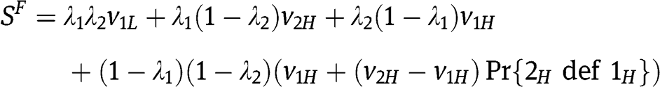
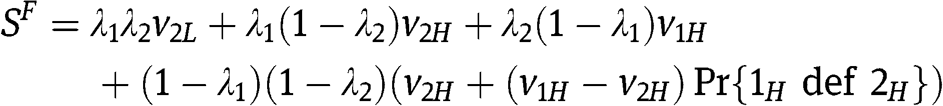
We evaluate  as the difference between the social surplus
  generated by the FPA minus the bidders’ rents
  :
:  . Thus, we need to derive
  and
and  :
:
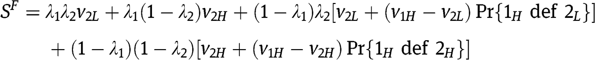

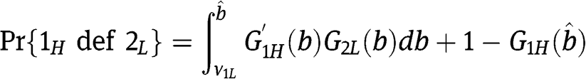
in which  def
def  , for
, for  , is the probability that
  wins when he faces type
  .
.
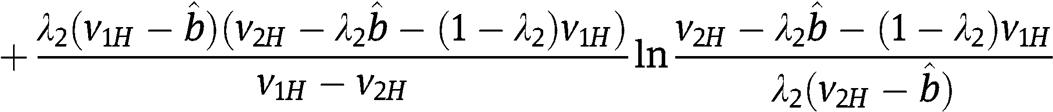
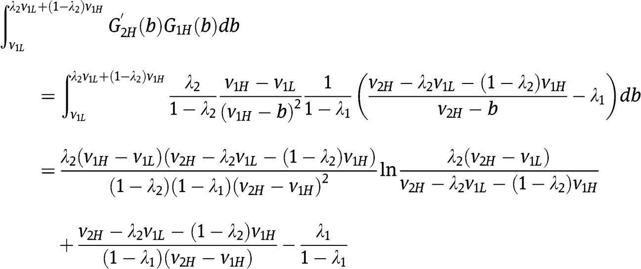
In order to derive  def
def  , for the case that
  , we need to evaluate
and using  in
in  we find
  . Hence

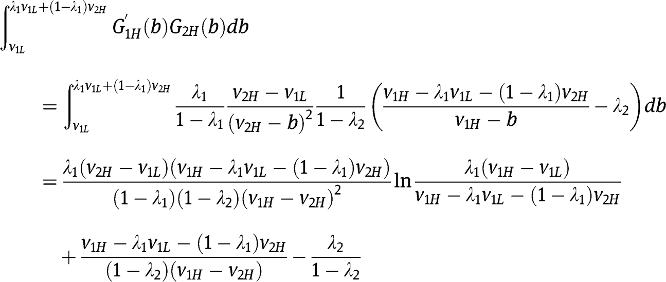
In order to derive  def
def  , for the case that
  , we need to evaluate

and using  in
in  we find
  . Hence
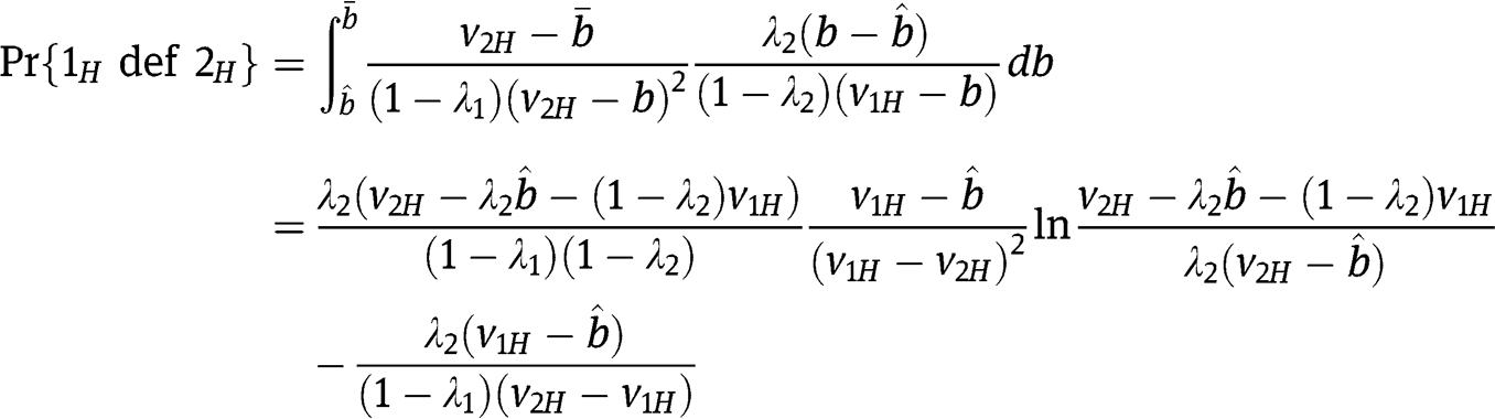
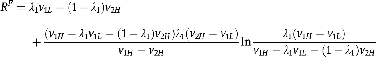
Now we can evaluate  :
:

An expression for  is found by solving eq. [2]:
![[15]](/document/doi/10.1515/bejte-2012-0014/asset/graphic/bejte-2012-0014_eq15.png)
with

The BNE of Proposition 1(ii) when  (footnote 10)

In order to derive  , for the case that
  , we need to evaluate
Now we can evaluate  :
:
![[16]](/document/doi/10.1515/bejte-2012-0014/asset/graphic/bejte-2012-0014_eq16.png)
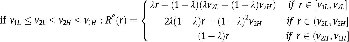
The BNE in Proposition 1(iii)

For the case that  we need to evaluate
  def
def  , which is equal to
Now we can evaluate  :
:
Proof of Lemma 1
Given  and
and  , when
  Proposition 1(ii) (footnote 10) applies and reveals that types
  bid as in the benchmark symmetric setting, whereas
 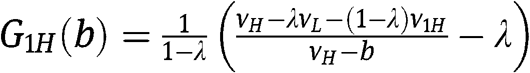 and
and  with support
  , in which
  . It is simple to see that both
  and
and  are decreasing with respect to
  for any
  , and this implies that
  and 2H are both more aggressive, in the sense of first-order stochastic dominance, the larger is
  in
in  .31 Given that
![[17]](/document/doi/10.1515/bejte-2012-0014/asset/graphic/bejte-2012-0014_eq17.png)
we infer that  is increasing in
  .
.
When  , Proposition 1(iii) applies and reveals that types
  bid as in the benchmark symmetric setting, whereas
 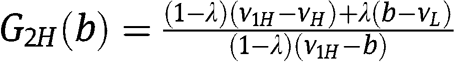 for any
 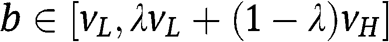 . Since
  is strictly increasing in
  for any
 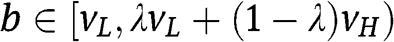 , we infer that 2H is less aggressive, in the sense of first-order stochastic dominance, the larger is
  . Using again eq. [17], after replacing
  with
with  and
and  with
with  , it follows that
  is strictly decreasing with respect to
  .
.
Proof of Proposition 4
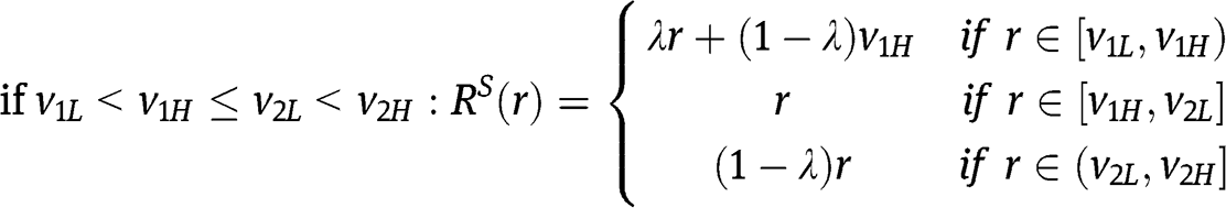
The proof when [9] or [10] is satisfied
The proofs for these results are provided in the text.
The proof when [11] is satisfied
Since  when [9] is satisfied and
  and
and  are continuous functions of the valuations, it follows that
  if
if  and
and  is close to
  .
.
The proof when [12] is satisfied
Recall from our final remark in Section 3.2.2 that in the BNE described by Proposition 1(ii) the highest valuation bidder does not always win. Conversely, the efficient allocation is always achieved in the SPA. Therefore a sufficient condition for  is that the aggregate bidders’ rents in the FPA,
  , are (weakly) larger than the rents in the SPA,
  . Indeed, we show that
  in region B if
  by proving that
  for any profile of values in B. Since
  , Proposition 1(ii) applies and thus the aggregate bidders’ rents in the FPA are
  with
with  . On the other hand, the bidders’ rents in the SPA are
  . Hence, the inequality
  reduces to
  . From eq. [15] we obtain
  with
with  . Therefore
  boils down to
  and (after squaring – notice that
  in B) ultimately to
  . Given
  and
and  , we find that
  , which is positive in region B.
For valuations in region C, that is such that  , we show that
  if [12] is satisfied. As above, the bidders’ rents in the FPA are
  with
with 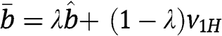 . However, the rents in the SPA in region C are
  , and the inequality
  reduces to
  . Using again
  we see that
  boils down to
  and, after squaring – notice that
  – ultimately to
![[18]](/document/doi/10.1515/bejte-2012-0014/asset/graphic/bejte-2012-0014_eq18.png)
We prove that this inequality holds for each  by verifying that the left-hand side of [18] is positive both at
  and at
  . At
. At 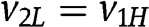 , the left-hand side in [18] reduces to
  which is positive since (i) it is increasing in
  ; (ii) has value
  at
at  . At
. At 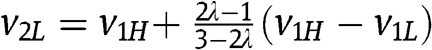 , the left-hand side in [18] reduces to
 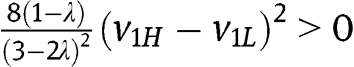 .
.
Proof for the case of distribution shift
In the case of shift,  and
and  . If
. If  , then
  and
and  . As a consequence,
  reduces to
  . If
. If  , then this inequality is satisfied for any
  ; if instead
  , then the inequality is violated for
  and it holds if and only if
  .
.
If  , then
  and
and  . As a consequence,
  reduces to
  . In order for this inequality to be satisfied by an
  larger than
  it is necessary that
  .
.
Proof of the claim in Section 4.3 about the approximation of our discrete setting using a continous model
Suppose that  and consider
  such that
  ; let
; let  be close to zero. If
  are continuously differentiable c.d.f.s which approximate well our discrete setting, then
  ,
,  ,
,  , and
, and  by definition of
  . We show that [14] is violated at
  by deriving a contradiction if the inequality
  holds for each
  . Indeed, if this condition were satisfied then
  , but we know that
  .32 In other terms,
  needs to be small for
  , and [14] requires that
  is smaller than
  for any x between
  and
and  . But since
  , it is necessary that
  grows substantially in
  , which is impossible given that
  is small.33
Proof of Proposition 5
The expression of  depends as follows on
  :
:
In the case of  , for instance,
  is increasing in
  , is increasing in
  , and is increasing in
  , thus
  . A similar argument applies in the other cases.
Proof of Proposition 6
Step 1 If  , then the optimal reserve price in the FPA belongs to
  .
.
First notice that if  , then bidding
  allows bidder 2 to win with certainty. Hence, no type of bidder 2 (or of bidder 1) bids above
  in equilibrium and
  for each
  . Second, if
  then bidder 1 does not participate in the auction. Bidder 2 participates, and bids r, if and only if
  . Therefore
  if
if  (both types of bidder 2 bid r), and
  if
if  (only type
  bids r).
Step 2 If  , then the optimal reserve price in the FPA belongs to
  .
.
The result follows from Steps 2.1 and 2.2 below.
Step 2.1 If we consider only values of r in  , then the optimal r is in
  .
.
Let bidders i and j be such that  (if
(if  , then we set
  ,
,  ). Thus
  is the type of bidder with valuation equal to
  .
.
From  and
and  it follows that
  . For r such that
  the BNE is such that types
  do not bid; types
  play mixed strategies, each with support
  , with
  , and c.d.f.s
![[19]](/document/doi/10.1515/bejte-2012-0014/asset/graphic/bejte-2012-0014_eq19.png)
Since both types  bid more aggressively as r increases in
  , it follows that
  is increasing with respect to r in the interval
  , and
, and  .
.
For r such that  , only type
  participates, and bids r. Thus
  is increasing with respect to r in the interval
  , and
, and  . Hence the optimal r in
  belongs to
  ■
■
Notice that when  , Step 2.1 implies immediately that the optimal r belongs to
  . Therefore in the following of the proof, we assume that
Step 2.2 If we consider only values of r in  , then the optimal r is
Given  , we need to consider two cases:
  and
and  .
.
Step 2.2.1 If  , then
  is increasing with respect to r in the interval
  .
.
When  the BNE is similar to the BNE described in Proposition 1(ii), with
  replaced by r: type
  does not bid; types
  play mixed strategies with support
  for
for  ,
,  for
for  ,
,  for
for  , in which
  is the smaller solution to
![[20]](/document/doi/10.1515/bejte-2012-0014/asset/graphic/bejte-2012-0014_eq20.png)
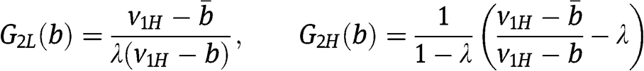
and  . The c.d.f.s for the mixed strategies of
  are, respectively:
Since  is the smaller solution to eq. [20] and the left-hand side in eq. [20] is increasing in r, it follows that
  is increasing in r and also
  is so. Hence, it is immediate that an increase in r induces both types
  and
and  to bid more aggressively. The same result holds for type
  as well since
  for
for  , and both
  and
and  are decreasing in r. Therefore
  is increasing in r. ■
Step 2.2.2 If  , then
  is increasing with respect to r in the interval
 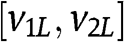 .
.
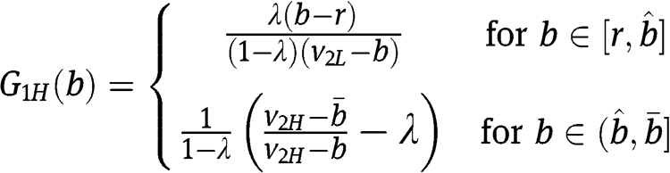
When  the BNE is similar to the BNE described in Proposition 1(iii), with
  replaced by r: type
  does not bid; type
  bids r; types
  play mixed strategies with the same support
  , in which
  and the c.d.f.s are given by eq. [19], with
  ,
,  . Hence
  is increasing in r. ■
Proof of Proposition 7
For the case of  , see the arguments immediately after the statement of Proposition 7. When
  , first notice that
 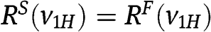 ,
,  . For instance, if
  (similar results are obtained if
  ) then
  because given
  , in both auctions the object is not sold when
  , and in the other states of the world the winning bidder pays
  . In case that
  , we have
  because in both auctions the object is sold if and only if
  . On the other hand,
  (
( ) is equal to the expected revenue in the FPA (in the SPA) when
  , and we know from Proposition 4 (condition [9]) that
  , unless
  .
.
References
Cantillon, E. 2008. “The Effect of Bidders’ Asymmetries on Expected Revenue in Auctions.” Games and Economic Behavior62:1–25.10.1016/j.geb.2006.11.005Search in Google Scholar
Cheng, H. 2006. “Ranking Sealed High-Bid and Open Asymmetric Auctions.” Journal of Mathematical Economics42:471–98.10.1016/j.jmateco.2006.05.008Search in Google Scholar
Cheng, H.2010. “Asymmetric First Price Auctions with a Linear Equilibrium.” Mimeo.Search in Google Scholar
Cheng, H. 2011. “Asymmetry and Revenue in First-Price Auctions.” Economics Letters111:78–80.10.1016/j.econlet.2010.12.004Search in Google Scholar
Doni, N., and D.Menicucci. 2012a. “Revenue Comparison in Asymmetric Auctions with Discrete Valuations.”http://www1.unifi.it/dmd-old/persone/d.menicucci/WpAsymmetric.pdf.10.1515/bejte-2012-0014Search in Google Scholar
Doni, N., and D.Menicucci. 2012b. “Information Revelation in Procurement Auctions with Two-Sided Asymmetric Information.” Journal of Economics and Management Strategy forthcoming.Search in Google Scholar
Fibich, G., and N.Gavish. 2011. “Numerical Simulations of Asymmetric First-Price Auctions.” Games and Economic Behavior73:479–95.10.1016/j.geb.2011.02.010Search in Google Scholar
Fibich, G., and A.Gavious. 2003. “Asymmetric First-Price Auctions – A Perturbation Approach.” Mathematics of Operations Research28:836–52.10.1287/moor.28.4.836.20510Search in Google Scholar
Fibich, G., A.Gavious, and A.Sela. 2004. “Revenue Equivalence in Asymmetric Auctions.” Journal of Economic Theory115:309–21.10.1016/S0022-0531(03)00251-5Search in Google Scholar
Gavious, A., and Y.Minchuk. 2013. “Ranking Asymmetric Auctions.” Mimeo. International Journal of Game Theory forthcoming. DOI: 10.1007/s00182-013-0383-9.10.1007/s00182-013-0383-9Search in Google Scholar
Gayle, W., and J.-F.Richard. 2008. “Numerical Solutions of Asymmetric, First Price, Independent Private Values Auctions.” Computational Economics32:245–75.10.1007/s10614-008-9125-7Search in Google Scholar
Kaplan, T. R., and S.Zamir. 2012. “Asymmetric First Price Auctions with Uniform Distributions: Analytical Solutions to the General Case.” Economic Theory50:269–302.10.1007/s00199-010-0563-9Search in Google Scholar
Kirkegaard, R. 2012a. “A. Mechanism Design Approach to Ranking Asymmetric Auctions.” Econometrica80:2349–64.10.3982/ECTA9859Search in Google Scholar
Kirkegaard, R.2012b. “Ranking Asymmetric Auctions: Filling the Gap Between a Distributional Shift and Stretch.”http://www.uoguelph.ca/~rkirkega/BetweenShiftStretch.pdf.Search in Google Scholar
Klemperer, P. 1999. “Auction Theory: A Guide to the Literature.” Journal of Economic Surveys13:227–86.10.1111/1467-6419.00083Search in Google Scholar
Lebrun, B. 1998. “Comparative Statics in First Price Auctions.” Games and Economic Behavior25:97–110.10.1006/game.1997.0635Search in Google Scholar
Lebrun, B. 2002. “Continuity of the First-Price Auction Nash Equilibrium Correspondence.” Economic Theory20:435–53.10.1007/s001990100227Search in Google Scholar
Lebrun, B. 2009. “Auctions with Almost Homogeneous Bidders.” Journal of Economic Theory144:1341–51.10.1016/j.jet.2008.11.013Search in Google Scholar
Li, H., and J.Riley. 2007. “Auction Choice.” International Journal of Industrial Organization25:1269–98.10.1016/j.ijindorg.2006.10.003Search in Google Scholar
Marshall, R. C., M. J.Meurer, J.-F.Richard, and W.Stromquist. 1994. “Numerical Analysis of Asymmetric First Price Auctions.” Games and Economic Behavior7:193–220.10.1006/game.1994.1045Search in Google Scholar
Marshall, R. C., and S. P.Schulenberg2003. “Numerical Analysis of Asymmetric Auctions with Optimal Reserve Prices.” Mimeo, Department of Economics, Penn State University, State College, PA.Search in Google Scholar
Maskin, E., and J.Riley1983. “Auction with Asymmetric Beliefs.” Discussion Paper n. 254, University of California-Los Angeles.Search in Google Scholar
Maskin, E., and J.Riley. 1985. “Auction Theory with Private Values.” American Economic Review75:150–5.Search in Google Scholar
Maskin, E., and J.Riley. 2000a. “Asymmetric Auctions.” Review of Economic Studies67:413–38.10.1111/1467-937X.00137Search in Google Scholar
Maskin, E., and J.Riley. 2000b. “Equilibrium in Sealed High Bid Auctions.” Review of Economic Studies67:439–54.10.1111/1467-937X.00138Search in Google Scholar
Myerson, R. B. 1981. “Optimal Auction Design.” Mathematics of Operations Research6:58–73.10.1287/moor.6.1.58Search in Google Scholar
Plum, M. 1992. “Characterization and Computation of Nash-Equilibria for Auctions with Incomplete Information.” International Journal of Game Theory20:393–418.10.1007/BF01271133Search in Google Scholar
Vickrey, W. 1961. “Counterspeculation, Auctions, and Competitive Sealed Tenders.” Journal of Finance16:8–37.10.1111/j.1540-6261.1961.tb02789.xSearch in Google Scholar
- 1
This result contrasts with a claim in Maskin and Riley (1985) for the case in which the only deviation from a symmetric setting is given by unequal high valuations [this claim is reproduced in Klemperer (1999)]. However, for this case, Maskin and Riley (1983) agree with our ranking between the FPA and the SPA.
- 2
In fact, the latter result is known, and in more general settings, since Maskin and Riley (2000a).
- 3
As we mentioned above, these results hold if the probability of a low value is the same for each bidder. In Doni and Menicucci (2012a), we study the case in which the probabilities of a low value for the two bidders are different. We also partially extend our results to a setting in which each bidder’s valuation has a three-point support.
- 4
Doni and Menicucci (2012b) study a procurement setting in which the auctioneer privately observes the qualities of the products offered by the suppliers and needs to decide how much of the own information on qualities should be revealed to suppliers before a (first score) auction is held. Our results on the comparison between the FPA and the SPA contribute to determine the best information revelation policy for the auctioneer.
- 5
Cheng (2010) studies the environments such that each bidder’s equilibrium bidding function is linear.
- 6
Cheng (2011) employs the same setting of Maskin and Riley (1983) in order to show that in some special cases the asymmetry increases the expected revenue in the FPA, unlike in the examples studied in Cantillon (2008).
- 7
In order to circumvent this problem, some authors apply numerical methods: see Fibich and Gavish (2011), Gayle and Richard (2008), Li and Riley (2007), and Marshall et al. (1994).
- 8
A very similar idea appears in Lebrun (2002), in the auction he denotes with
 .
. - 9
For instance, 1H bids according to the uniform distribution on
 with α < 1 and close to 1.
 - 10
In the case that
 (which occurs if and only if
  ), 2L bids
  and
and  , thus
  and
and 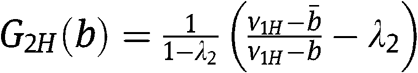 for each
  .
. - 11
In a setting with continuously distributed valuations, Maskin and Riley (2000a) identify an analogous BNE and provide the intuition we describe here and after Proposition 2. In addition, Maskin and Riley (1983) identify the BNE we describe in Proposition 1 for the case of
 . Thus Proposition 1 is a new result for the case in which
  and [3] is violated.
 - 12
This fact may appear similar to the main message in Cantillon (2008), but in fact in our analysis the benchmark symmetric setting is fixed, whereas in Cantillon (2008) it is not.
- 13
Obviously, an analogous result holds if
 is kept fixed and
  is allowed to vary.
 - 14
Lebrun (1998) considers a setting with continuously distributed valuations and assumes that the valuation distribution of one bidder changes into a new distribution which dominates the previous one in the sense of reverse hazard rate domination (the support is unchanged). He show that, as a consequence, for each bidder the new bid distribution first-order stochastically dominates the initial bid distribution and thus the expected revenue increases.
- 15
In particular,
 for any small deviation from the symmetric setting, that is when
  and
and  are close to zero, but
  and/or
  .
. - 16
Since they assume
 , Maskin and Riley (1983) do not consider the various cases covered in our Proposition 4, and they do not have the results in our Lemma 1 and Propositions 5 to 7.
 - 17
Proposition 1 still holds even though
 violates our assumption
  . However, when
  the Vickrey tie-breaking rule is needed also if
  .
. - 18
This similarity should not be overstated, since the uniform distribution on
 gives zero probability to
  , unlike the uniform distribution on
  . See Section 4.3 for a discussion on the relationship between the results in our model and in the rest of the literature.
 - 19
If we set
 , then
  , which violates the assumption
  , but nevertheless
  is the c.d.f. of the equilibrium mixed strategy of bidder 2 when
  .
. - 20
This effect appears also in Example 3 in Maskin and Riley (2000a).
- 21
Maskin and Riley (2000a) prove the same result under slightly stronger assumptions.
- 22
In fact, we can prove that a small shift reduces
 as it has a zero first-order effect on the bidding of types
  , but induces
  to bid less aggressively.
 - 23
A similar result is obtained if we fix
 and set
  ,
,  , with
  . For the case of a large
  , [3] is satisfied and thus
  . If instead
  is close to 1, then [11] reveals that
  . On the other hand, Kirkegaard (2012b) proves that
  if
if  is such that
  is convex and logconcave,
  is such that
  and
and  is not much larger than 1.
 - 24
Kirkegaard (2012b) provides an economic interpretation of this order linked to the relative steepness of the demand function of bidder 1 with respect to the demand function of bidder 2.
- 25
We are grateful to one referee for suggesting the main ideas in this paragraph.
- 26
We thank one referee for suggesting to investigate the effect of reserve prices.
- 27
Kirkegaard (2012a) shows that if [13] and [14] are satisfied, then the FPA is superior to the SPA for any common reserve price smaller than
 , that is such that it allows participation of some type of the weak bidder. Asymmetric auctions with reserve prices are analyzed, using numerical techniques, also in Gayle and Richard (2008), Li and Riley (2007), and Marshall and Schulenberg (2003). In these papers, introducing a reserve price tipically either makes the SPA superior to the FPA (even though the reverse result holds when there is no reserve price) or reduces the revenue advantage of the FPA over the SPA. The latter results are consistent with our results in this section.
 - 28
In fact, a small shift reduces
 as in the case of binary supports (see footnote 22), mainly because it induces type
  to bid less aggressively.
 - 29
We do not provide here the proof for the case in which [3] is satisfied since the BNE in that case is similar to a BNE in Maskin and Riley (2000a): see footnote 11. Doni and Menicucci (2012a) provide a complete proof.
- 30
Notice that
 given [7].
 - 31
Precisely, if
 , then
  and
and  given
given  first-order stochastically dominate, respectively,
  and
and  given
given  .
. - 32
In case that
 we can prove that [13] is violated.
 - 33
Actually, [14] can be replaced in Theorem 1 in Kirkegaard (2012a) with a weaker condition, inequality [8] in Kirkegaard (2012a), but our argument establishes that also such a condition is violated. Furthermore, our argument does not require that
 and
and  have binary supports, consistently with the results we describe in Section 5.2 for the case in which supports are three-point sets.
©2013 by Walter de Gruyter Berlin / Boston
Articles in the same Issue
- Masthead
- Masthead
- Advances
- Dependence and Uniqueness in Bayesian Games
- Monopolistic Signal Provision†
- Multi-task Research and Research Joint Ventures
- Transparent Restrictions on Beliefs and Forward-Induction Reasoning in Games with Asymmetric Information
- A Simple Bargaining Procedure for the Myerson Value
- On the Difference between Social and Private Goods
- Optimal Use of Rewards as Commitment Device When Bidding Is Costly
- Labor Market and Search through Personal Contacts
- Contributions
- Learning, Words and Actions: Experimental Evidence on Coordination-Improving Information
- Are Trust and Reciprocity Related within Individuals?
- Optimal Contracting Model in a Social Environment and Trust-Related Psychological Costs
- Contract Bargaining with a Risk-Averse Agent
- Academia or the Private Sector? Sorting of Agents into Institutions and an Outside Sector
- Topics
- Poverty Orderings with Asymmetric Attributes
- Dictatorial Mechanisms in Constrained Combinatorial Auctions
- When Should a Monopolist Improve Quality in a Network Industry?
- On Partially Honest Nash Implementation in Private Good Economies with Restricted Domains: A Sufficient Condition
- Revenue Comparison in Asymmetric Auctions with Discrete Valuations