
A gap-filling algorithm selection strategy for GRACE and GRACE Follow-On time series based on hydrological signal characteristics of the individual river basins
-
Hamed Karimi
 ,
Siavash Iran-Pour
,
Siavash Iran-Pour

Abstract
Gravity recovery and climate experiment (GRACE) and GRACE Follow-On (GRACE-FO) are Earth’s gravity satellite missions with hydrological monitoring applications. However, caused by measuring instrumental problems, there are several temporal missing values in the dataset of the two missions where a long gap between the mission dataset also exists. Recent studies utilized different gap-filling methodologies to fill those data gaps. In this article, we employ a variety of singular spectrum analysis (SSA) algorithms as well as the least squares-harmonic estimation (LS-HE) approach for the data gap-filling. These methods are implemented on six hydrological basins, where the performance of the algorithms is validated for different artificial gap scenarios. Our results indicate that each hydrological basin has its special behaviour. LS-HE outperforms the other algorithms in half of the basins, whereas in the other half, SSA provides a better performance. This highlights the importance of different factors affecting the deterministic signals and stochastic characteristics of climatological time series. To fill the missing values of such time series, it is therefore required to investigate the time series behaviour on their time-invariant and time-varying characteristics before processing the series.
1 Introduction
Gravity Recovery And Climate Experiment (GRACE), as a joint mission between the National Aeronautics and Space Administration (NASA) and Deutsches Zentrum für Luft- und Raumfahrt (DLR), was launched in March 2002 and ended its science mission in October 2017. The GRACE satellite mission aimed to monitor time-variable gravity field of the Earth (Tapley et al. 2004). The mission measured Earth’s mass changes due to hydro-climatological variations such as groundwater storage changes (Syed et al. 2008, Landerer and Swenson 2012, Feng et al. 2013), ice melting (Chambers et al. 2007, Chen et al. 2007, Nahavandchi et al. 2015), Glacial Isostatic Adjustment (Peltier 2004, Chambers et al. 2010, Wahr and Zhong 2013), etc. After decommission of GRACE, the GRACE Follow-On (GRACE-FO) mission, as a collaboration of NASA and GeoForschungsZentrum (GFZ), was launched on 22 May 2018. The GRACE-FO satellite mission is similar to its predecessor GRACE, though employed more advanced measuring instrumentations such as laser interferometry.
The main temporal resolution of GRACE and GRACE-FO in time-variable gravity field recovery (level-2 and level-3 dataset) is 30 days. However, because of several instrumental problems in both missions, the dataset suffers from missing values. In particular, there is about one-year data gap between GRACE and GRACE-FO. This temporal gap starts from July 2017 and ends in May 2018. Several recent research works have tried to fill the missing values in the GRACE and GRACE-FO time series and the long gap between them.
Rietbroek et al. (2014) used GNSS-derived loading inversion technique to bridge the gaps within GRACE satellite mission data series, where three methods were employed: (1) GPS-I, that is based on GNSS inverting data and additionally constrained over the ocean area by a new regularization method, (2) GPS-C, which is a constrained GNSS solution where additional correction parameters were applied to GNSS data and (3) using seasonal gap-filler method by fitting a trend and a seasonal signal to the data series to bridge the gaps. In evaluation of these methods, the third approach outperformed the others, while GPS-C showed a lower Root Mean Square Error (RMSE) compared to GPS-I. Li et al. (2020) implemented different data-driven techniques to reconstruct (1992-2002) and predict (2017- 2018) GRACE-like gridded Total Water Storage Changes (TWSC) using the climate inputs. They used the combination of data-driven methods, such as Principal Component Analysis (PCA) (Wold et al. 1987), Independent Component Analysis (ICA), Least Squares (LS) (Durbin and Watson 1992), Seasonal and Trend decomposition using Loess (STL), Artificial Neural Network (ANN), autoregressive exogenous (ARX), Multiple Linear Regression (MLR) and additional dataset, such as precipitation, land surface temperature, climate indices, and Sea Surface Temperature (SST) data. In that work, the authors found that ARX and ANN methods work better than MLR algorithm in simulation of the target variables, although because of overfitting problems, they are not robust enough for prediction. Furthermore, they indicated that PCA-LS-MLR is the most robust combination method for prediction and reconstruction of GRACE-like TWSC over all river basins.
Several studies employed other existing satellite missions for the recovery of time-variable gravity field. Among those works, Satellite Laser Ranging (SLR) geodetic observations provide lower degrees of spherical harmonic coefficients of the Earth’s gravity field. Sośnica et al. (2015) recovered time-variable Earth gravity field through SLR observations through up to nine geodetic satellites: LAGEOS-1, LAGEOS-2, Starlette, Stella, AJISAI, LARES, LARES, Larets, BLITS, and Beacon-C. In their research, they showed that low-degree coefficients can be derived from SLR observations which carry good information about large-scale mass transport in the Earth system.
Low Earth Orbiter (LEO) satellites, equipped with an accelerometer, star camera tracker, and geodetic GNSS receiver, can be employed to recover time-variable gravity field. The European Space Agency Earth Explorer mission Swarm is one of these constellations. Swarm Satellite mission consists of three satellites. A pair of them (Swarm-Alpha and Swarm-Charlie) fly side-by-side in a circular, near-polar orbit with an initial altitude and inclination of 450 km and 87.4. The separation between the satellites is around 1–1.5 in the direction of east-west, in longitude (equivalent to approximately 10 sec delay in orbit). The higher satellite (Swarm-Bravo) flies in a circular and near-polar orbit as well, where its altitude and inclination are respectively 530 km and 86.8, and its right ascension of ascending node is close to that of the two other satellites (Friis-Christensen et al. 2008). Jäggi et al. (2016) used the Celestial Mechanics Approach to recover the time variable and static gravity field from Swarm kinematic orbit. They analysed the effect of severe ionosphere activity on precise orbit determination of the Swarm satellite mission. Moreover, they compared their results with the gravity field recovered from GRACE where they concluded that the Swarm satellite mission can recover long-wavelength time-variable gravity signals (up to degree 20).
Lück et al. (2018) used three methods to fill several types of artificial gaps of single, 3 and 18 months. Those methods included the following: (1) interpolating existing monthly GRACE solutions, (2) using monthly Swarm solutions, (3) using the CTAS (directly estimating constant, trend, and annual and semi-annual signal terms) Swarm solution. In their research, in most cases, the third method outperformed the first and second approaches, although it depended on the length of the gap. In the case of single-month or three-month gaps, the first method showed better performance, while the third approach outperformed the others in 18-month gap scenario. It is of important to mention that several previous studies indicated that Swarm has the capability to recover time-variable gravity field of the Earth at lower spherical harmonic degrees (up to d/o 12), i.e., coarser spatial resolution with more noise. Their results showed that trend and annual variations and seasonal components of mass changes can be retrieved from the kinematic orbit of the Swarm mission. However, in this way, there is no benefit to use accelerometer data and kinematic baseline from Swarm satellite missions in gravity inversion; therefore, only GPS-derived kinematic orbit has been utilized for the Earth’s gravity recovery. It should be mentioned here that the GPS antenna on Swarm spacecraft is 8-channel antenna and cannot collect GPS data more than a particular amount; this is an important problem and limitation in precise orbit determination of Swarm satellite mission, especially for the kinematic orbit of the Swarm satellites and consequently for the gravity recovery from the kinematic orbit (ESA 2014, Zangerl 2014, Jose van den IJssel 2015, van den IJssel 2016). Therefore, the gravity field derived from Swarm kinematic orbit cannot substitute the gravity field derived from GRACE and GRACE-FO satellite missions. In fact, because of Swarm coarse spatial resolution and its high level of noise in the lower level data (kinematic orbits), it is preferable to seek a robust mathematical method to bridge the missing values in GRACE and GRACE-FO time series and the long gap between them. For more details, see Bezděk et al. (2016) and Da Encarnação et al. (2016, 2019, 2020).
Forootan et al. (2020) used ICA method to fill the gaps between GRACE and GRACE-FO and the long gap between them. In their study, using ICA, they merged GRACE TWSC with the low spatial resolution TWSC from Swarm, where the aim was to bridge the gaps and missing values and improve the spatial resolution of Swarm TWSC. They employed two approaches in their study, where the first approach was based on the reconstruction of Swarm dataset in the spatial domain and the second approach implemented the reconstruction in the temporal domain. Their results showed that the gap-filling by use of the ICA-based method and merging GRACE and Swarm gravity field dataset has a good performance. In their evaluation, the second approach in the temporal domain outperformed the first approach in the spatial domain.
Yi and Sneeuw (2021) employed SSA to fill the missing values in GRACE and GRACE-FO dataset and the long gap between them. Their work made use of a methodology based on a gap-filling method through SSA in an iteration. This approach is the so-called zero-filling SSA which was proposed by Kondrashov and Ghil (2006). In their research study, they used the dataset of GRACE and GRACE-FO in the spectral domain, i.e., spherical harmonic coefficients of the time variable gravity field for the global solution.
There are several techniques to use SSA to forecast and fill the missing values in time series. These techniques are based on the reconstruction of time series from the original signals, regardless of the noise (Golyandina and Zhigljavsky 2013). However, Khazraei and Amiri-Simkooei (2019) proposed Monte Carlo SSA algorithm, introduced by Allen and Smith (1996), to differentiate between the oscillation parts of a time series including noise through decomposition. The algorithm employs Least Squares-Variance Component Estimation (LS-VCE) to estimate noise model parameters and generates surrogate data using Cholesky decomposition.
Rodrigues and De Carvalho (2013) provided a recurrent imputation method (RIM) based on a weighted average between forecast and hindcast, to bridge time series gaps and missing values. Mahmoudvand and Rodrigues (2016) introduced a new algorithm for gap-filling of a time series, where the method was based on RIM, although it uses bootstrap resampling and a given weighting scheme by sample variances. These two estimates are combined to produce a unique estimation for missing values. Least Squares-Harmonic Estimation (LS-HE) is, on the other hand, a parametric and stationary method for time series analysis, developed by Amiri-Simkooei (2007) and Amiri-Simkooei et al. (2007). This method as a generalized form of the classic Least-Squares Spectral Analysis (LSSA) considers a general linear trend and also the stochastic model of the time series. Moreover, Amiri-Simkooei and Asgari (2012) developed the multivariate LS-HE (MLS-HE), where they implemented their method on time series of total electron content (TEC) in the ionosphere. They detected several significant signals in the time series of TEC, such as diurnal and annual signals with periods of 24/n hours and 365.25/n days (n = 1, 2 …), along with their higher harmonics and their modulated variants.
In summary, several recent studies focused on using external dataset and different methodologies to fill the missing values and long gaps in time-variable gravity field of GRACE and GRACE-FO satellite missions. Our study, however, aims to evaluate and compare the performance of three main methods in gap-filling of the missing values in GRACE and GRACE-FO time series and prediction of the long gap between the two missions. Our focus in this research work is on a few hydrological basins where the special behaviours of each basin may play an important role in the gap-filling procedure. To this end, we assign six scenarios of artificial gaps. The algorithms are implemented in five large water catchments and one sub-catchment. The case studies are selected from various regions of the world that have different hydrological behaviours to reflect the essential application of different techniques for data gap-filling in hydrological dataset, e.g. GRACE and GRACE-FO time series. For this purpose, as it was mentioned earlier, we choose six case studies that are (i) Amazon basin, (ii) Congo river basin, (iii) Gavkhouni (or Gavkhuni) sub-basin, (iv) Aravalli basin, (v) Rhine river basins, and (vi) Tigris river basin. To have more information about the selected study areas, the reader is referred to subsection 3.2. The performance of the aforementioned methods on each artificial gaps is assessed in this research, where a kind of inter-validation is conducted for filling the real gaps. In the Amazon catchment, an additional dataset of the Swarm time variable gravity field is also employed for validation.
The main contribution and novelty of this study are to use the signal characteristics of each individual catchment learnt from the gap-filling of the artificial gaps, to fill the original gaps in the time-series. In this way, it is expected that the hydrological characteristics of each case study are taken into account for the data gap-filling of that specific area which influences the selection procedure of the gap-filling algorithm. We believe that our research work can contribute to any other research field where the characteristics of the signals can be employed for prediction and gap-filling of the missing values in a time series.
This article is organized as follows. In Section 2, we present the methodologies employed for the data gap-filling of our research. Section 3 introduces data and study areas of the work, while the results are discussed in Section 4. Finally, Section 5 summarizes and concludes the research.
2 Methodology
Three different gap-filling methods are introduced in this section: (i) RIM-SSA, (ii) zero-filling SSA, and (iii) LS-HE.
First, SSA is introduced as a general method for time series analysis. Then, the recurrent singular-spectrum procedure is presented as a time-series gap-filling approach. Afterward, we describe an iterative zero-filling SSA algorithm. At the end, LS-HE mathematical formulation for filling the time series missing values is discussed.
2.1 Singular Spectrum Analysis (SSA)
SSA is a data-driven non-stationary method for signal processing and time series analysis. SSA and PCA are both based on Karhunen–Loeve theory of random fields and of stationary random processes, where SSA uses Singular Value Decomposition (SVD) of a Hankel matrix, constructed from the main time series (Ghil et al. 2002). This method can be implemented on time series to decompose it in temporal patterns such as trend, oscillatory signals, and random noise. In the Hankel matrix, the diagonal elements equal together, i.e. i + j = const → a ij = const, and are constructed from the time series in the embedding step. After embedding and applying SVD on the Hankel matrix, the modes are grouped, extracted from eigentriples into interpretable signals such as the annual and seasonal signals and random noise. Eventually, the time series is reconstructed from the grouped modes by diagonal averaging of the Hankel matrix. Here, we describe SSA in two steps: decomposition and reconstruction (Golyandina and Zhigljavsky 2013).
Consider a time series y = (y 1, … y m ) T by the length of m, which m > 2 and y is a non-zero series, that is, there is at least one i such that y i ≠ 0. Let L(1 < L < N) be an integer number as the length of the window and K = m − L + 1 (the number of lagged vectors).
2.1.1 First stage: Decomposition
Step 1: Embedding
At the start, the time series should be arranged in a Hankel matrix form, where the original time series is mapped into a sequence of lagged vectors. Consider matrix X as a Hankel matrix, constructed from the main time series. This matrix would be formed as follows:
where Y i are so-called lagged vectors. There are K lagged vectors in the Hankel matrix. The length of each lagged vectors equals L. The L-trajectory matrix, constructed from the original time series is
The lagged vectors are the columns of the trajectory matrix. Each rows and columns are a subset of the original time series (Golyandina and Zhigljavsky 2013).
Step 2: SVD
This step deals with the implementation of SVD on the trajectory matrix, where the matrix is decomposed to the left and right patterns and singular values. The implementation of SVD on matrix X results in:
The previous equation consists of U , the left pattern, V the right pattern, and S , the singular values including the square roots of eigenvalues of S = XX T , i.e. λ 1, … λ L . The aforementioned decomposition can be written as follows:
where
2.1.2 Second stage: reconstruction
Step 3: Eigentriple grouping
In this step, the power of each mode is calculated as:
In this way, each mode is associated to its corresponding eigentriple with its calculated power. The time series can then be divided into d groups, where each of these groups has the power of P i , i ∈ {1, …, d}. Now, considering the modes up to a special power r < d, it is possible to reconstruct the original time series. Here, one can interpret that the individual modes greater than a specific power value are taken as signals, and therefore, the remaining modes are noise and have no contribution to the reconstructed time series. Therefore, the reconstructed time series gets the following form:
The aforementioned grouping is called elementary grouping.
Step 4: Diagonal averaging
From the nature of Hankelized trajectory matrices related to each eigentriples, a special procedure should be applied to a Hankel matrix to extract the modes or reconstruct the time series from a trajectory matrix. This is called diagonal averaging. Using this method, the trajectory matrix is transformed into a time series. Diagonal averaging operator is defined as follows (Golyandina and Zhigljavsky 2013, Rodrigues and De Carvalho 2013):
where
Hence, we can decompose the time series to d modes, related to each eigentriple or reconstruct the time series from the first to the rth mode. For more information, the reader refers to Golyandina and Zhigljavsky (2013), Rodrigues and De Carvalho (2013).
2.2 Recurrent singular-spectrum-based procedure
2.2.1 Recurrent forecast method
To fill the gaps in a time series, different methods to predict the missing values are being introduced. First of all, a singular-spectrum-based forecasting method is explained, and in the next step a RIM is provided.
Let y i as an out-of-sample data forecast, as a linear combination of l − 1 preceding observations:
for a suitable choice of coefficients a = (a 1, …, a i−1) T . To choose a suitable set of the aforementioned coefficients, consider the matrix constituted by eigenvectors of XX T , suitably subdivided as follows:
where U 1 consists of the first L − 1 components of eigenvectors corresponding to the signal, and u 1 contains the last components of those eigenvectors. Similarly, U 2 and u 2 are defined, although they correspond to the remainder d − r components associated with the noise. According to Golyandina and Osipov (2007), the above-mentioned coefficients are computed as follows:
where ‖.‖ denotes the Euclidian norm,
Based on this algorithm, the one-step-ahead forecast of out-of-sample data series can be written as a linear combination of l − 1 reconstructed values of the time series:
where the coefficients are taken from equation (11) and the tildes are used to denote reconstructed time series from the original and oscillatory signals. In general, for further forecasts of out-of-sample values, the following algorithm is proposed:
for 2, …, L − 1 steps-ahead, respectively. In this article, the notation
2.2.2 RIM
In this subsection, a recurrent method to fill the missing values in a time series of interest is introduced. This method is based on a weighted average between forecast and hindcast, where the forecast is performed according to subsection 2.2.1. Furthermore, the hindcast values are computed analogously, although in the reverse order of the time series. That means, hindcast is in fact a forecast, but in reverse order (Rodrigues and De Carvalho 2013).
Consider the time series y = (y 1, …, y m ) T with a block of k sequential missing values. Let the decomposition of the time series as the following equation to known and missing values:
where n* = m − n − k. y n is the n-vector of known values before the missing values, y k is a k-vector of missing values and y n* is the n*-vector of known values after missing values. By prediction and estimation of missing values, the filled time series will be as follows:
with
where
where
denotes the weighting coefficients related to the forecasts achieved by recurrent forecast algorithm. For more details about this method, the readers refer to Rodrigues and De Carvalho (2013).
In this contribution, we use several weighting schemes. In the next subsection, these weighting strategies are described in more detail.
2.2.2.1 Linear weighting scheme
Linear weighting strategy is based on the distribution of the missing values in a time series. In fact, the method makes use of the closeness of missing values to the dataset for forecast or hindcast; i.e. if a missing value is closer to the forecast value, the weighting number for forecast is greater than the weighting value for hindcast and vice versa. The weighting function is defined as (Rodrigues and De Carvalho 2013, Mahmoudvand and Rodrigues 2016):
2.2.2.2 Modified weighting strategy
In some cases, the number of data points of a time series used to forecast does not equal the number used for hindcast. In this way, the number of data points to forecast or hindcast would affect the prediction, and therefore, the linear weighting scheme is not appropriate. In such cases, Rodrigues and De Carvalho (2013) suggested a new weighting scheme to address this problem. This weighting strategy makes use of:
Or in vector notation:
In a special case, where the number of observations used to forecast and hindcast is equal (n = n*), the equation above becomes the linear weighting scheme of equation (21).
2.2.2.3 Stochastic weighting
In this part, we introduce an innovative stochastic weighting scheme for the data gap-filling by SSA. If we have some information about the stochastic properties of time series, it is possible to define a weight function based on the variance of the data used to forecast or hindcast. For this purpose, at first, the variance of forecast and hindcast should be derived according to error propagation law. What it means is based on recurrent forecast (or hindcast) method. In this method, if l is considered as the window size of the trajectory matrix in SSA, l − 1 number of coefficients is calculated and multiplied into the l − 1 data series before the missing value (in the case of forecast). Therefore, it is easy to use error propagation law to calculate the variance of the forecast value (and also the hindcast value in the same way). In order to reach this goal, consider
where Q y is the covariance matrix of the vector y. Therefore, according to error propagation law, we will have:
Note that
From the discussion earlier, it is possible to calculate the variance of each forecast of the missing values. Consider y f as the n-vector of forecasts for missing values and y h as the n-vector of hindcasts (in one gap). Now, using the covariance matrix of y f , y h we can take a Best Linear Unbiased Estimation (BLUE) of the missing values. Let Q yf and Q yh be the covariance matrices of y f and y h , their diagonal elements are computed by using the error propagation law, equation (28). Therefore, we have:
The model of observation equations are:
where E{.} and D{.} are expectation and dispersion operators, respectively. By a combination of (33) and (34), the Gauss–Markov model will be as follows:
Based on the Least-Squares theory, we have
Then,
As we can see, equation (37) is a weighted average. This equation is used to predict the missing values by use of stochastic weighting.
2.2.2.4 Linear-stochastic weighting
In this subsection, an innovative combination of linear weighting methods based on data distribution in a time series with stochastic properties of missing values is discussed. The approach is utilized to have a combined weighted average between forecast and hindcast, where the weighted average is according to equation (37), but the covariance matrices are different as follows:
1 Linear part
2 Stochastic part
For the final covariance matrix, we have
Using the covariance matrices for forecast and hindcast according to equation (42) and (43), the LS estimation of
2.3 Zero-filling SSA
Here, we employ a gap-filling algorithm based on an iterative SSA procedure. The zero-filling SSA method has been introduced by Kondrashov and Ghil (2006) and was later employed by Zscheischler and Mahecha (2014). The method provided in these studies is based on setting zero or mean values of time series for the missing values. In the literature mentioned above, an iterative gap-filling procedure was proposed to fill the missing values in a time series. At first, the missing values are replaced by zero (or mean values of the time series). In the second step, in the inner loop, SSA is implemented on the zero-filled time series. After the reconstruction of the time series, extracted from SSA, the missing values (zero values) are then replaced by the values from the first mode. In this loop, the temporal correlation (in a univariate time series) or spatiotemporal correlation (in a spatiotemporal dataset) is utilized to validate the gap-filling procedure where a threshold for the loop is introduced.
In this study, 2.5% of RMSE is used as a criterion. That means when the new RMSE is smaller than 2.5% of the previous RMSE, the inner loop is stopped. After replacing the missing values, SSA is applied to the new time series and the loop continues until it reaches the threshold. The outer loop aims to separate the signal from the noise. After using the first mode in the inner iteration and filling the gaps, the reconstruction of the data is now continued by using the second mode added to the reconstructed missing values from the first mode. In the next iteration of the outer loop, another mode is added to reconstruct the time series. The added modes may represent the noise; therefore, the procedure may increase the RMSE value. If RMSE increases, we stop the outer iteration. For more details, you can refer to the study by Kondrashov et al. (2010).
2.4 LS-HE
LS-HE is a parametric stationary method based on the LS principles and Fourier expansion of a time series, developed by Amiri-Simkooei (2007). In this way, a Gauss-Markov model is considered for the time series, which consists of a functional model and a stochastic model. There is a duality between these two parts that the periodic signals in a time series such as trend, annual, semi-annual, and diurnal frequencies are captured by the functional model, while different types of noise in the time-series such as white noise, flicker noise, or random walk noise are taken in the stochastic part.
Consider a time series in a m-vector y. It can be expressed as a summation of a linear trend and some periodic terms such as in the following equation:
In a matrix notation, it could be written as:
The equation earlier is called the Gauss–Markov model, where A is the design matrix, for example, contains the linear trend terms, and A k consists of two columns related to the frequency ω k of the periodic terms:
with a k , b k , and ω k are the (un)known real numbers. In fact, if the frequencies ω k are known, the harmonic coefficients a k and b k can be estimated based on the linear LS principles, although in most cases, we do not have exact information about the frequencies existing in a time series. In this situation, in addition, to estimate the harmonic coefficients according to the current linear LS model, the frequencies should be also detected and estimated in the time series. This is the so-called harmonic estimation and is the task of LS-HE.
To find a set of frequencies ω 1, …, ω q , and a particular value of q in equation (45), the following null and alternative hypothesis is considered (to start, set i = 1):
versus
The detection and validation of ω i are performed in two steps:
Step I: In the first step, the frequency ω i and the corresponding design matrix A i are looked for. The procedure follows the solution to the minimization problem:
where
with
with
Step II: In order to test the null hypothesis against the alternative hypothesis H o, the following statistic is used:
where
where α is the level of significance in the central Fisher test. After the detection of unknown frequencies, the design matrix is formed by a linear trend and periodic signals. For the sake of brevity, we name the final design matrix A. The harmonic coefficients are then estimated based on the linear least-squares principles:
Based on the two steps earlier, the periodic terms and sinusoidal frequencies in the time series are detected. After detection and validation of the functional model, i.e. finding the frequencies of interests in the time series, the missing values in the time series are estimated using a suitable detected functional model. In fact, the detected frequencies are introduced to the functional model and the time argument is updated by adding the time argument of missing values into the design matrix. Afterwards, the reconstructed time series, including (now) filled-values, is estimated through the following equation:
where A
new is the new design matrix, including rows associated with the missing values, although the same column size as A in equation (54) is kept. In this way,
3 Data and study areas
3.1 Data
3.1.1 GRACE L3 data
In this contribution, we use JPL mascon level-3 grid dataset RL06 version 2 processed by NASA Jet Propulsion Laboratory (JPL). This dataset is derived from mass concentration (mascon) solution based on surface spherical cap basis functions rather than spherical harmonics. The solutions aim to make improvements by using a priori information derived from near-global geophysical models and prevent striping in the solutions (Watkins et al. 2015). In order to reduce the leakage error and separation of land area from oceans, a Coastline Resolution Improvement (CRI) filter was applied to JPL-mascon RL06 v02 dataset (Wiese et al. 2016). The grid time series consist of GRACE and GRACE-FO data. GRACE-FO processing strategy is similar to GRACE, although there are a few differences in sensor analysis and processing of the GRACE-FO data. For more details see Landerer et al. (2020).
The dataset is available to download from https://podaac.jpl.nasa.gov/dataset/TELLUS_GRAC-GRFO_MASCON_CRI_GRID_RL06_V2.
3.1.2 Swarm L2
Another dataset, used in this article, is the spherical harmonic coefficients derived from the kinematic orbit of the Swarm satellite mission. Several analysis centers provide gravity field solutions from Swarm. In this study, we use the spherical harmonic coefficients, provided by the Astronomical Institute, Czech Academy of Science (ASU), where the processing strategy is based on Bezděk et al. (2016). The gravity field was derived from 3 Swarm satellites (Swarm-Alpha, Swarm-Charlie, and Swarm-Bravo), through the acceleration approach (Guo et al. 2015). The product is solved up to spherical harmonic coefficients degree and order of 40, although they are only significant up to degree and order 15 (Bezděk et al. 2016 and Da Encarnação et al. 2016, 2019, 2020). The solutions can be downloaded from http://www.asu.cas.cz/∼bezdek/vyzkum/geopotencial/index.php.
3.2 Study areas
We choose five river catchments and one sub-catchment, where our introduced gap-filling methodologies are implemented. The time series are in the form of TWSC, extracted from JPL mascon grid data introduced in Section 3. One of the main reasons for selection of these study areas is that we tend to capture different hydrological signal characteristics by the use of different methods explained in the previous section. The selected case studies are five hydrological basins and a sub-basin with different behaviours either stationary or non-stationary from various regions that are distributed around the globe. The study areas of this research article are as follows:
Amazon basin is located in South America with geographical coordinates of about 20S-5N in latitude and 80W-55W in longitude (Figure 1a).
Congo river basin in Central Africa is a sedimentary basin of the Congo river. Its geographical extension is about 15S-10N in latitude and 12E-35E in longitude (Figure 1b).
Gavkhouni (or Gavkhuni) sub-basin is located in the Iranian Plateau in Central Iran, where Gavkhouni wetland is the terminal basin of the Zayandehrud River, east of the city of Isfahan. Its geographical coordinates are limited to about 31N–34N in latitude and 50E–54E in longitude (Figure 1c).
Aravalli (India) basin which is located in India that its geographical coordinates are limited to about 2N–28N in latitude and 68E–76E in longitude (Figure 1d).
Rhine river basin is a catchment of Rhine river, located in the west of central Europe and its geographical coordinates are limited to about 46N–52N in latitude and 4E–12E in longitude (Figure 1e).
Tigris river basin is located in Western Asia by the geographical coordinates of about 33N–39N
in latitude and 39E–48E in longitude (Figure 1f).
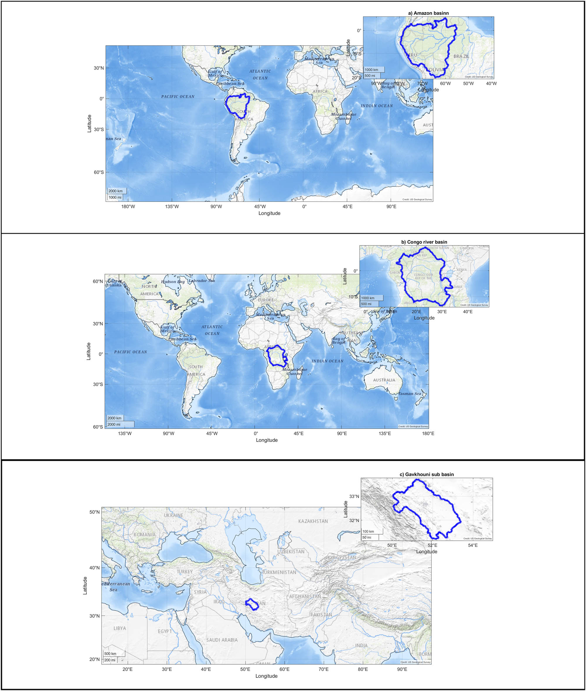
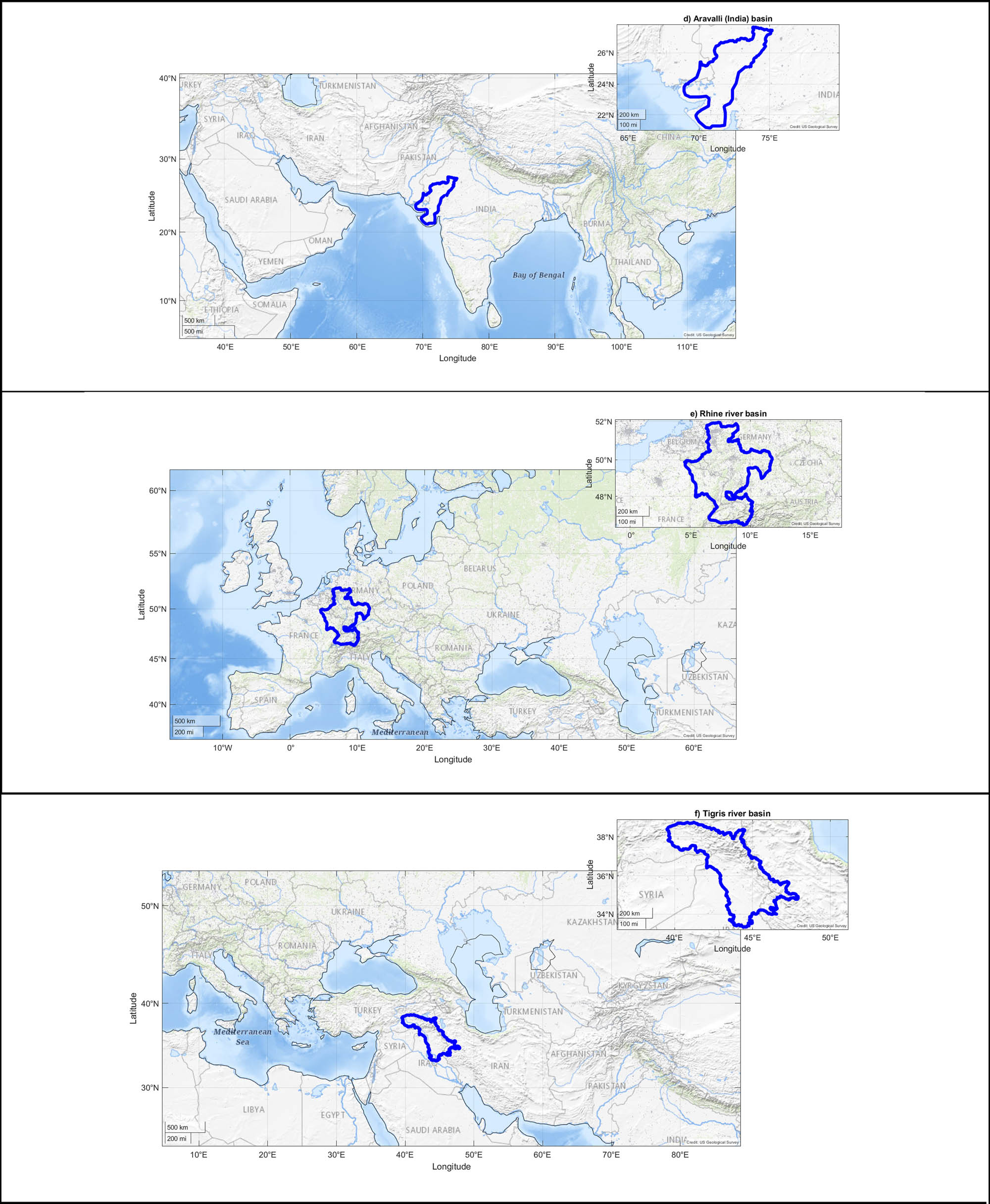
Geographical boundaries of (a) Amazon, (b) Congo, (c) Gavkhouni, (d) Aravalli, (e) Rhine, and (f) Tigris river basins.
Amazon basin is located in South America with a tropical climate regime. Congo basin, the basin of Congo River, located in west-central Africa, is the world’s second-largest river basin (next to that of Amazon). Its climate is approximate as the same as the Amazon basin i.e. tropical. In fact, these two basins have almost similar climatological behaviour. The Rhine river basin including German Rhine, French Rhine, Dutch Rijn, Celtic Renos, and Latin Rhenus, lies in Central Europe with humid and mild climate. The Aravalli Mountain Range, located in South Asia, has a complex climate regime. Hence, its climate cannot be generalized into a single exact climatological behaviour. However, the dominant climate in the selected location in this research work is arid, steppe and hot. Gavkhouni sub-basin and Tigris river basin, located in the Middle-East, southwestern Asia, have arid and semi-arid climate regime; however, the higher part of Tigris river basin could be categorized as subtropical.
4 Results
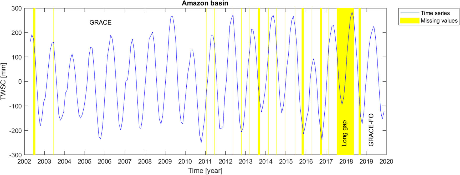
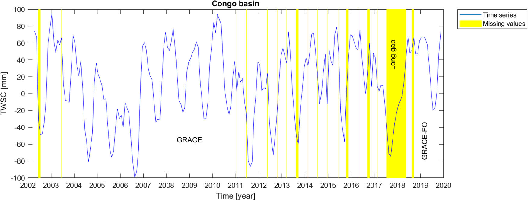
Mascon level-3 data series provides information about time variable total water storage on the continental scale and ocean areas. Originating from time-to-time instrumental problems in GRACE and GRACE-FO measuring devices, the time series include missing values, causing sparse temporal gaps in GRACE and GRACE-FO dataset. The most serious gap in the time series, however, is the long gap between GRACE and GRACE-FO satellite missions. In order to report the data gaps, GRACE missing months are respectively June and July 2002, June 2003, January and June 2011, May and October 2012, March, August and September 2013, February, July and December 2014, June, October and November 2015, April, September and October 2016 and February 2017. Then, there is a long 11-months gap between GRACE and GRACE-FO missions, which started on July 2017 and ended in June, 2018. GRACE Follow-On gaps happened in August and September 2018.
Concerning the gap-filling problem, we here employ several methodologies, described in Section 2. However, lacking reliable information for validation of our gap-filling procedures, we design different artificial gap scenarios, similar to the gaps which exist in the main time series. These scenarios also include a long artificial gap, similar to the long gap between GRACE and GRACE-FO, to simulate the real long gap between two satellite missions. It should be mentioned here that we only make use of GRACE time series to validate the gap-filling methodologies using artificial gaps. Those artificial gaps are chosen between the years 2003 and 2011 in which there is no real gap, and the time span is long enough to derive the main signal signatures. The real gaps outside the validation time span are then filled from the results of the artificial gap-filling procedure where the best filling performance for each specific gap type is taken.
Our artificial gaps include the following:
Short gaps:
at the start of time series (2 data points gap);
at the end of time series (2 data points gap);
sparse gaps in the middle of time series (8 data points gap);
on a peak in the middle of time series (3 data points gap);
on a valley in the middle of time series (5 data points gap).
A long gap similar to the gap between GRACE and GRACE-FO:
- In the middle of the time series (13 data points gap)
It would be of importance to note that our short gaps scenarios consist of different schemes including “continuous a few months” and “sparse individual” missing values in the time series. On the other hand, based on the fact that there is a long gap (about one year) between GRACE and GRACE-FO measurements, we also simulate this gap scenario via a long artificial gap in the middle of time series where there is no data gap, i.e. between the years 2003 and 2011. Concerning these two sectors of missing values, i.e. short gaps and a long gap in the GRACE and GRACE-FO time series, we tackle the issue in two different manners; one is the scenarios for different types of short artificial gaps as previously mentioned, and another one is the long artificial gap.
To review our gap-filling approaches, we employ:
SSA – Linear weighting,
SSA – Stochastic weighting,
SSA – Linear + Stochastic,
SSA – Equation (22) weighting,
LS-HE,
Zero-filling SSA.
It should be noted that the length of the window through SSA data processing is set to 23 months which was determined by the trial-and-error method. However, wherever there are not enough data to choose 23-month window for the case of modified weighting strategy, we select 12-month window length as the other optimal case in our trial-and-error. This selection illustrates the capability of the modified weighting strategy in choosing various window lengths. It is noticeable that the number of data points used for gap-filling procedure depends on the length of the window in RIM-SSA (subsection 2.2.1, equation (9)). Moreover, the level of significance α in Fisher test through LS-HE analysis; i.e., equation (53) is considered α = 0.01.
The focus of this research study is on analysing the time series of GRACE and GRACE-FO in the scales of the hydrological catchment. In fact, we expect that different catchments on the globe show different regional and local hydro-climatological behaviours. To this end, it might be of interest to localize time series analysis, i.e. the gap-filling procedure. We expect that through the global analysis, some information in the data related to a specific catchment or basin might be lost. Therefore, in this contribution, we focus on the performance of a few gap-filling algorithms for particular basins where their particular temporal hydro-climatological variations may play a role.
The results for the selected river basins of this research work are provided in the form of Root Mean Square Error (RMSE), shown in the tables below. In those tables, the numbers identified with “*” and “**” respectively show the maximum and minimum RMSE. Those values are brought for the long gap scenario as well as the mean of the short gap scenarios.
Through our results from the error values for different artificial gap scenarios, for each catchment or the sub-catchment, we fill the real gaps by the best methodology, i.e. the approach which provides the minimum average RMSE for similar short artificial gap scenarios. Similarly, the long gap between GRACE and GRACE-FO is filled by using the methodology that provides minimum RMSE for the artificial long gap. We also try to validate the results in the Amazon basin where coarse-resolution Swarm satellite mission dataset is available. That comparison is employed for the long gap between GRACE and GRACE-FO missions.
As it can be seen in Table 1 for the Amazon catchment, according to RMSE values, for both short artificial gaps and long gap, LS-HE outperforms the other methods. In Table 2, related to Congo basin, for both short and long artificial gaps, the SSA-based methods have the best performance in comparison to LS-HE. For the short gap, the minimum RMSE value happens for the linear weighting scheme, while for the long gap, it is for the modified weighting strategy (equation (22)). Similarly, for Gavkhouni sub-basin in Table 3, the SSA-based algorithms perform better than the LS-HE method. In contrast, in the Aravalli basin (Table 4), the LS-HE method outweighs the SSA algorithms, based on RMSE values. Considering the Rhine river basin in Table 5, the LS-HE algorithm also outperforms the SSA-based methods for the gap-filling of both short- and long-gap scenarios. In Table 6, related to the Tigris river basin, SSA-based methods outperform the LS-HE approach. In fact, a linear weighting scheme for short gaps and zero-filling SSA for long gap are the selected gap-filling algorithms in this river basin.
RMSE of different gap-filling approaches for different artificial gap scenarios (in millimetres)
| Methodology scenario | Linear | Stochastic | Linear + stochastic | Equation (22) | LS-HE | Zero SSA |
|---|---|---|---|---|---|---|
| At the start of time series (2 data points gap) | 20.4685 | 20.4685 | 20.4685 | 20.4685 | 20.6374 | 25.1746 |
| At the end of time series (2 data points gap) | 80.5358 | 76.0217 | 74.2130 | 72.7237 | 2.8036 | 29.9342 |
| Sparse gaps in the middle of time series (8 data point gaps) | 41.8615 | 42.9797 | 41.6217 | 42.7612 | 16.3608 | 32.4756 |
| On a peak in the middle of time series (5 data points gap) | 18.4899 | 19.1665 | 18.2766 | 15.6434 | 45.0657 | 29.2166 |
| On a valley in the middle of time series (5 data points gap) | 22.1782 | 23.3190 | 22.6671 | 23.5007 | 33.4065 | 28.6969 |
| A long gap in the middle of time series (13 data points gap) | 50.9374 | 53.1432 | 50.3081 | 48.2266 | **41.6504 | *53.1898 |
| Mean (short gaps) | *36.7068 | 36.3911 | 35.4494 | 35.0195 | **23.6548 | 29.0996 |
Case study: Amazon catchment.
RMSE of different gap-filling approaches for different artificial gap scenarios (in millimetres)
| Methodology scenario | Linear | Stochastic | Linear + stochastic | Equation (22) | LS-HE | Zero SSA |
|---|---|---|---|---|---|---|
| At the start of time series (2 data points gap) | 5.2338 | 5.2338 | 5.2338 | 5.2338 | 41.7297 | 12.6932 |
| At the end of time series (2 data points gap) | 18.2123 | 21.1500 | 20.7382 | 20.4522 | 35.7006 | 42.9766 |
| Sparse gaps in the middle of time series (8 data point gaps) | 24.3505 | 25.1604 | 24.4127 | 23.9361 | 10.8862 | 20.3583 |
| On a peak in the middle of time series (5 data points gap) | 17.1544 | 38.9118 | 26.1971 | 33.1270 | 20.9514 | 73.2415 |
| On a valley in the middle of time series (5 data points gap) | 21.4280 | 13.6125 | 20.7505 | 22.6881 | 54.7953 | 34.5355 |
| A long gap in the middle of time series (13 data points gap) | 44.7085 | 45.1826 | 44.6203 | **43.7533 | 48.0585 | *57.6334 |
| Mean (short gaps) | **17.2758 | 20.8137 | 19.4665 | 21.0875 | 32.8127 | *36.7610 |
Case study: Congo catchment.
RMSE of different gap-filling approaches for different artificial gap scenarios (in millimetres)
| Methodology scenario | Linear | Stochastic | Linear + Stochastic | Equation (22) | LS-HE | Zero SSA |
|---|---|---|---|---|---|---|
| At the start of time series (2 data points gap) | 32.2532 | 32.2532 | 32.2532 | 32.2532 | 44.8030 | 8.8139 |
| At the end of time series (2 data points gap) | 13.6297 | 13.6954 | 13.8634 | 16.8283 | 29.0280 | 6.8683 |
| Sparse gaps in the middle of time series (8 data point gaps) | 40.7343 | 42.8314 | 39.6545 | 38.1363 | 26.2551 | 17.6618 |
| On a peak in the middle of time series (5 data points gap) | 25.2618 | 53.3889 | 41.1724 | 12.6306 | 30.6888 | 54.3657 |
| On a valley in the middle of time series (5 data points gap) | 9.4875 | 16.6917 | 8.5431 | 15.5566 | 10.3816 | 31.1998 |
| A long gap in the middle of time series (13 data points gap) | **17.8644 | 34.9699 | 19.6581 | 18.2800 | 27.6050 | *43.3225 |
| Mean (short gaps) | 24.2733 | *31.7721 | 27.0973 | **23.0810 | 28.2313 | 23.7819 |
Case study: Gavkhouni sub–catchment.
RMSE of different gap-filling approaches for different artificial gap scenarios (in millimetres)
| Methodology scenario | Linear | Stochastic | Linear + stochastic | Equation (22) | LS-HE | Zero SSA |
|---|---|---|---|---|---|---|
| At the start of time series (2 data points gap) | 25.5799 | 25.5799 | 25.5799 | 25.5799 | 44.6704 | 59.2802 |
| At the end of time series (2 data points gap) | 35.5045 | 34.5419 | 35.2623 | 32.1965 | 34.0011 | 22.8984 |
| Sparse gaps in the middle of time series (8 data point gaps) | 61.1407 | 65.6547 | 64.8060 | 68.5364 | 73.4819 | 43.7642 |
| On a peak in the middle of time series (5 data points gap) | 50.8645 | 80.3509 | 56.7596 | 38.0011 | 48.5929 | 31.2840 |
| On a valley in the middle of time series (5 data points gap) | 49.0850 | 65.4309 | 62.0002 | 56.4806 | 4.9388 | 105.8602 |
| A long gap in the middle of time series (13 data points gap) | 45.1861 | *66.2811 | 64.7680 | 57.1327 | **37.6942 | 59.2191 |
| Mean (short gaps) | 44.4349 | *54.3117 | 48.8816 | 44.1589 | **41.1370 | 52.6174 |
Case study: Aravalli catchment.
RMSE of different gap-filling approaches for different artificial gap scenarios (in millimetres)
| Methodology scenario | Linear | Stochastic | Linear + stochastic | Equation (22) | LS-HE | Zero SSA |
|---|---|---|---|---|---|---|
| At the start of time series (2 data points gap) | 41.3717 | 41.3717 | 41.3717 | 41.3717 | 4.8838 | 88.8826 |
| At the end of time series (2 data points gap) | 17.4140 | 14.0056 | 13.9402 | 18.1710 | 13.9398 | 70.2588 |
| Sparse gaps in the middle of time series (8 data point gaps) | 31.5832 | 31.9249 | 31.6157 | 38.9355 | 36.8090 | 36.6027 |
| On a peak in the middle of time series (5 data points gap) | 20.2959 | 25.8769 | 24.8529 | 21.5425 | 40.9743 | 24.6808 |
| On a valley in the middle of time series (5 data points gap) | 46.1394 | 51.7295 | 51.2178 | 47.1480 | 33.1184 | 26.2067 |
| A long gap in the middle of time series (13 data points gap) | 21.5968 | 25.0890 | 24.1261 | 21.7165 | **19.7416 | *29.7169 |
| Mean (short gaps) | 31.3608 | 32.9817 | 32.5997 | 33.4338 | **25.9451 | *49.3263 |
Case study: Rhine river basin.
RMSE of different gap-filling approaches for different artificial gap scenarios (in millimetres)
| Methodology scenario | Linear | Stochastic | Linear + stochastic | Equation (22) | LS-HE | Zero SSA |
|---|---|---|---|---|---|---|
| At the start of time series (2 data points gap) | 32.7811 | 32.7811 | 32.7811 | 32.7811 | 66.3301 | 48.5389 |
| At the end of time series (2 data points gap) | 12.4195 | 12.7349 | 12.7380 | 14.4415 | 13.9039 | 27.5019 |
| Sparse gaps in the middle of time series (8 data point gaps) | 35.7467 | 45.6868 | 43.4379 | 34.6070 | 25.4082 | 52.8257 |
| On a peak in the middle of time series (5 data points gap) | 37.5673 | 26.6984 | 27.0401 | 29.2360 | 38.7588 | 28.1148 |
| On a valley in the middle of time series (5 data points gap) | 47.1061 | 101.7836 | 86.0735 | 57.4388 | 48.0503 | 21.6055 |
| A long gap in the middle of time series (13 data points gap) | 34.0266 | 45.5997 | 44.2745 | 41.3589 | *66.7102 | **24.8927 |
| Mean (short gaps) | **33.1242 | *43.9370 | 40.4141 | 33.7009 | 38.4903 | 35.7174 |
Case study: Tigris river basin.
To summarize the procedure, the missing values of GRACE and GRACE Follow-On are categorized in two types of gap scenarios, namely short gaps and a long gap scenario. According to the results in Tables 1–6 and the final results in Table 7, for each artificial gap scenario, a specific gap-filling method outperforms the others (i.e. minimum RMSE). Those results are then taken as the criteria for the gap-filling procedure. The results of the table also show that LS-HE is the most successful methodology among all, which may come from the fact that the total water storage anomaly from the GRACE and GRACE Follow-On data have dominant parametric and stationary behaviour. Studying the LS-HE method, one recognizes that the method is a parametric and stationary approach for time series analysis and signal processing. This fact may explain the results of Table 7, where in half of the cases LS-HE outperforms the other algorithms. However, it is likely that there are catchments and sub-catchments with non-stationary or even random behaviours. In this contribution, we have employed six types of gap-filling methodologies on six catchments and sub-catchments which may possess different behaviours.
The outperforming methodologies for the artificial short- and long-gap scenarios in different study areas
| Study area | Methodology by minimum RMSE | |
|---|---|---|
| Short gaps | Long gap | |
| Amazon | LS-HE | LS-HE |
| Congo | Linear SSA weighting | Equation (22) |
| Gavkhouni | Equation (22) | Linear SSA weighting |
| Aravalli | LS-HE | LS-HE |
| Rhine | LS-HE | LS-HE |
| Tigris | Linear SSA weighting | Zero-SSA |
Finally, we perform the gap-filling procedures on the real gaps of the GRACE and GRACE Follow-On data. For each scenario (i.e., short or long gaps) and for each river basin, the corresponding outperforming method from the studied artificial scenarios is chosen to fill the real data gaps. Figures 2–8 illustrate the results of the real (natural) data gap-filling procedure for TWSC time-series, expressed artificial gap-filling procedure, presented in the tables earlier. That means, for the real gaps in the Amazon catchment of Figure 2, LS-HE algorithm is utilized for the gap-filling of short and long data gaps. For the Congo catchment in Figure 3, we utilize SSA-based methods, i.e. linear weighting scheme and modified weighting strategy for gap-filling of short gaps and long gap, respectively. In the Gavkhouni sub-catchment of Figure 4 with its apparent change point around the year 2008, a modified weighting strategy and linear weighting scheme for gap-filling of short gap and long gap are, respectively, employed. For the Aravalli basin (Figure 5), we make use of LS-HE for data gap-filling for both short gaps and long gaps. That is again based on the results from the artificial gap-filling procedure, here from Table 4. In the Rhine river basin, shown in Fig. 6, LS-HE is the utilized method for the gap-filling procedure. Figure 7 represents the case in Tigris river basin, where we respectively employ linear weighting scheme and zero-filling SSA for gap-filling of the short and long gaps, based on the results from the artificial gap-filling scenarios for the basin. It might be of interest to note that Tigris TWSC time series shows similar behaviour to Gavkhouni sub-basin case, i.e. the alternation of amplitude and a change point around the year 2008. That may come from this fact that Tigris and Gavkhouni river basins are close to each other, both located in the Middle-East with almost similar climate regime and water management policy.
Time series of TWSC for Amazon catchment where the gaps were filled.
Time series of TWSC for Congo catchment where the gaps were filled.
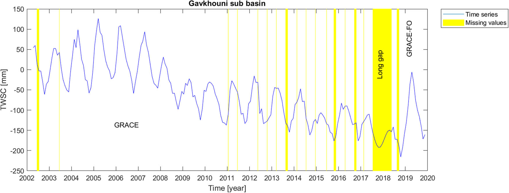
Time series of TWSC for Gavkhouni sub-catchment where the gaps were filled.
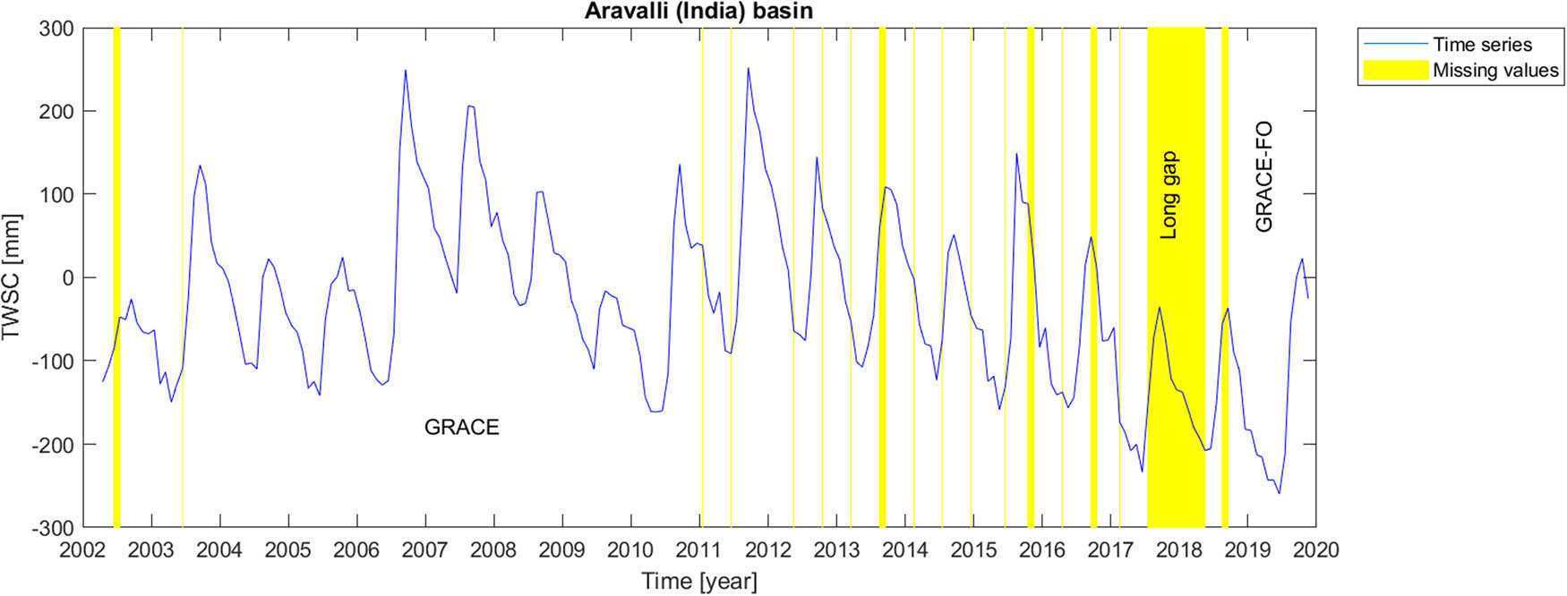
Time series of TWSC for Aravalli catchment where the gaps were filled.
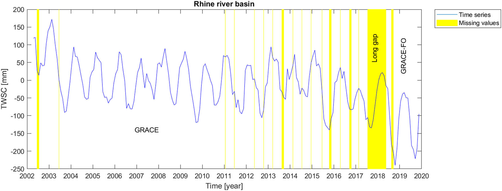
Time series of TWSC for Rhine river basin where the gaps were filled.
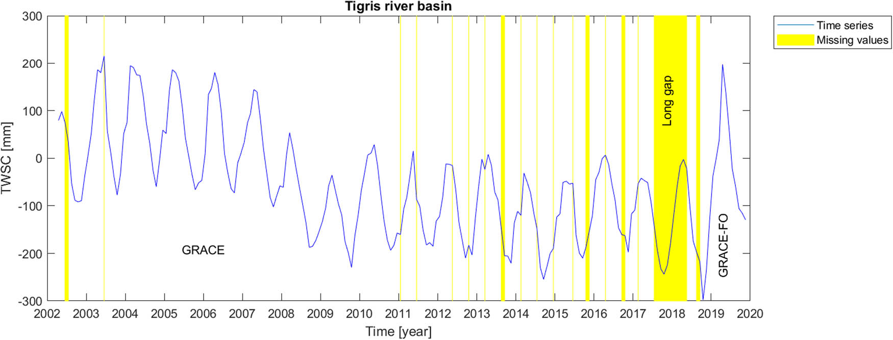
Time series of TWSC for Tigris river basin where the gaps were filled.
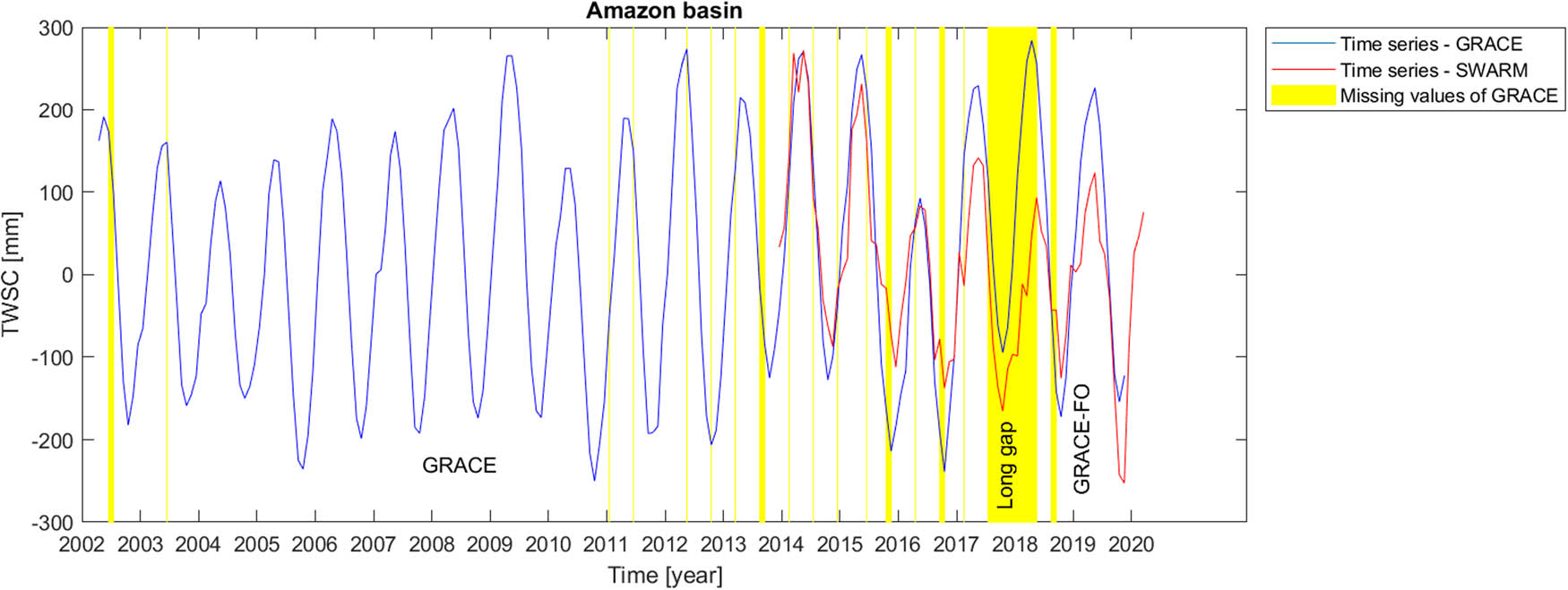
Time series of TWSC for Amazon catchment compared with the corresponding time series from Swarm satellite mission.
In this research work, we also make use of gravity field recovery derived from Swarm kinematic orbit to validate the result of our gap-filling procedure for the Amazon catchment. Because of the coarse spatial resolution of Swarm gravity field recovery, we only employ the data for the Amazon catchment, where the area and the hydrological signals are large enough to be studied by Swarm. The results of Figure 8 indicate a good correlation between our gap-filling procedure for the missing data between GRACE and GRACE-FO time series and the time series derived from the Swarm satellite mission. It should be also noted that we here focus on the visualized data correlation rather than the data match, since the data from those missions are processed in different ways and are not completely comparable.
It should be mentioned that, in this research study, we proposed a RIM-SSA weighting strategy to use the stochastic properties of the time series in the gap-filling procedure. However, this methodology did not provide a good performance compared to the other methods. The poor performance of our RIM-SSA approach might be influenced by the fact that we only used the uncertainties provided by the mascon level-3 dataset where the error propagation law was employed to propagate the uncertainties for the estimation of the missing value. We expect that a more realistic stochastic model of the dataset would increase the performance of the method.
5 Summary and conclusion
In this research study, several methodologies have been employed to fill the missing values in the GRACE and GRACE-FO time series. The methodologies have been implemented on the JPL mascon level-3 data series of TWSC derived from GRACE and GRACE-FO satellite missions, where the datasets are provided in a grid form of the spatial resolution of 0.5° and temporal resolution of 1 month. Here, we have focused on the analysis of the datasets for 6 study areas, named Amazon, Congo, Gavkhouni, Aravalli, Rhine and Tigris. Because of the lack of reliable datasets for validation of our gap-filling procedure, we have created artificial gaps in the time series similar to the original existing gaps in the GRACE and GRACE-FO datasets. In general, the gaps were categorized into two main scenarios: (i) different types of short gaps and (ii) a long gap. For each river basin, each gap scenario, and each gap-filling algorithm, we have formulated the error as RMSE derived from filling the artificial gaps. In this way, it was interesting to observe that each catchment or sub-catchment has shown a special behaviour. Therefore, based on the results from the artificial gap-filling procedures, a special gap-filling methodology for each river basin and each gap scenario, i.e. short gaps and long gap, has been employed for real data gap-filling. We found that in half of all cases of the artificial gaps, the LS-HE approach has outperformed the other gap-filling methods. We therefore think that those hydrological basins show a parametric and stationary behaviour, seen in the TWSC derived from the GRACE and GRACE-FO datasets. However, in several study areas and scenarios, the other methodologies outperformed a bit better or they may have also acceptable performance in comparison with the LS-HE algorithm. That may mean not all the river basins and study areas have dominant parametric and stationary behaviour.
As a result, we may conclude that if we want to fill the gaps and missing values in the GRACE and GRACE-FO time series, it would be preferable to create artificial gaps for each study area and detect its temporal behaviour; afterward, based on the results from the artificial gap-filling procedures, we may employ the most appropriate method, i.e. the least RMSE scenario, to fill the missing values. That might be, in particular, a valid statement for filling the long gap between GRACE and GRACE-FO.
For future research studies, we propose to employ the methods described in this article for more study areas, where a more diverse selection of the hydrological basins and their corresponding behaviours can be analysed. Furthermore, one can think of other methodologies for time series analysis and signal processing to improve the gap-filling procedure. Those methodologies may differ in performance speed and the way they model the signals. It is also important to mention that in the current research study, we did not make use of external datasets for our gap-filling procedures. Obviously, one can also think of using other data sources such as hydrological models or GNSS Earth deformation information, in a so-called data fusion approach. That was, however, beyond the scope of our current research study, where we focused on a self-validating data gap-filling approach. Another outlook for the current study might be achieved through the improvement of the stochastic model of the time series where signals are tried to be separated from the noise. The employment of an appropriate functional model to identify the deterministic behaviour of the time series and a realistic stochastic model is expected to influence the performance of the gap-filling procedures.
Acknowledgments
The authors would like to take this opportunity to sincerely thank Jet Propulsion Laboratory (JPL) for providing free access to GRACE and GRACE-FO global mascon level-3 data products of this study.
-
Conflict of interest: Authors state no conflict of interest.
References
Allen, M. R. and L. A. Smith. 1996. “Monte Carlo SSA: Detecting irregular oscillations in the presence of colored noise.” Journal of Climate 9(12), 3373–404.10.1175/1520-0442(1996)009<3373:MCSDIO>2.0.CO;2Search in Google Scholar
Amiri-Simkooei, A. 2007. “Least-squares variance component estimation: theory and GPS applications.” Doctral Thesis. Delft University of Technology (TU Delft), The Netherlands.10.54419/fz6c1cSearch in Google Scholar
Amiri-Simkooei, A. and J. Asgari. 2012. “Harmonic analysis of total electron contents time series: methodology and results.” GPS Solutions 16(1), 77–88.10.1007/s10291-011-0208-xSearch in Google Scholar
Amiri-Simkooei, A., C. C. Tiberius, and P. J. Teunissen. 2007. “Assessment of noise in GPS coordinate time series: methodology and results.” Journal of Geophysical Research: Solid Earth 112(B7), B07413. 10.1029/2006JB004913.Search in Google Scholar
Bezděk, A., J. Sebera, J. Teixeira da Encarnação and J. Klokočník. 2016. “Time-variable gravity fields derived from GPS tracking of Swarm.” Geophysical Journal International 205(3), 1665–9.10.1093/gji/ggw094Search in Google Scholar
Chambers, D. P., J. Wahr, M. E. Tamisiea and R. S. Nerem. 2010. “Ocean mass from GRACE and glacial isostatic adjustment.” Journal of Geophysical Research: Solid Earth 115(B11), B11415. 10.1029/2010JB007530.Search in Google Scholar
Chambers, D. P., M. E. Tamisiea, R. S. Nerem and J. C. Ries. 2007. “Effects of ice melting on GRACE observations of ocean mass trends.” Geophysical Research Letters 34(5), L05610. 10.1029/2006GL029171.Search in Google Scholar
Chen, J., C. Wilson, B. Tapley, D. Blankenship and E. Ivins. 2007. “Patagonia icefield melting observed by gravity recovery and climate experiment. GRACE).” Geophysical Research Letters 34(22), L22501. 10.1029/2007GL031871.Search in Google Scholar
Da Encarnação, J. T., D. Arnold, A. Bezděk, C. Dahle, E. Doornbos, J. van den IJssel, et al. 2016. “Gravity field models derived from Swarm GPS data.” Earth, Planets and Space 68(1), 1–15.10.1186/s40623-016-0499-9Search in Google Scholar
Da Encarnação, J. T., P. Visser, D. Arnold, A. Bezdek, E. Doornbos, M. Ellmer, et al. 2020. “Description of the multi-approach gravity field models from Swarm GPS data.” Earth System Science Data 12(2), 1385–417.10.5194/essd-12-1385-2020Search in Google Scholar
Da Encarnação, J. T., P. Visser, D. Arnold, A. Bezdek, E. Doornbos, M. Ellmer, et al. 2019. “Multi-approach gravity field models from Swarm GPS data.”Search in Google Scholar
Durbin, J. and G. S. Watson. 1992. Testing for serial correlation in least squares regression. I. Breakthroughs in Statistics. New York: Springer, pp. 237–59.10.1007/978-1-4612-4380-9_20Search in Google Scholar
ESA’s Magnetic Field Mission SWARM. Accessed 20-Aug-2014.Search in Google Scholar
Feng, W., M. Zhong, J. M. Lemoine, R. Biancale, H. T. Hsu and J. Xia. 2013. “Evaluation of groundwater depletion in North China using the Gravity Recovery and Climate Experiment. GRACE) data and ground-based measurements.” Water Resources Research 49(4), 2110–8.10.1002/wrcr.20192Search in Google Scholar
Forootan, E., M. Schumacher, N. Mehrnegar, A. Bezděk, M. J. Talpe, S. Farzaneh, et al. 2020. “An iterative ICA-based reconstruction method to produce consistent time- variable total water storage fields using GRACE and Swarm Satellite data.” Remote Sensing 12(10), 1639.10.3390/rs12101639Search in Google Scholar
Friis-Christensen, E., H. Lühr, D. Knudsen and R. Haagmans. 2008. “Swarm–an Earth observation mission investigating geospace.” Advances in Space Research 41(1), 210–6.10.1016/j.asr.2006.10.008Search in Google Scholar
Ghil, M., M. Allen, M. Dettinger, K. Ide, D. Kondrashov, M. Mann, et al. 2002. “Advanced spectral methods for climatic time series.” Reviews of Geophysics 40(1), 3-1–3-41.10.1029/2000RG000092Search in Google Scholar
Golyandina, N. and A. Zhigljavsky. 2013. Singular spectrum analysis for time series. New York: Springer.10.1007/978-3-642-34913-3Search in Google Scholar
Golyandina, N. and E. Osipov. 2007. “The “Caterpillar”-SSA method for analysis of time series with missing values.” Journal of Statistical Planning and Inference 137(8), 2642–53.10.1016/j.jspi.2006.05.014Search in Google Scholar
Guo, J., K. Shang, C. Jekeli and C. Shum. 2015. “On the energy integral formulation of gravitational potential differences from satellite-to-satellite tracking.” Celestial Mechanics and Dynamical Astronomy 121(4), 415–29.10.1007/s10569-015-9610-ySearch in Google Scholar
Jäggi, A., C. Dahle, D. Arnold, H. Bock, U. Meyer, G. Beutler, et al. 2016. “Swarm kinematic orbits and gravity fields from 18 months of GPS data.” Advances in Space Research 57(1), 218–33.10.1016/j.asr.2015.10.035Search in Google Scholar
IJssel, JVD., Encarnação, J, Doornbos, E, Visser, P. 2015. Precise science orbits for the Swarm satellite constellation. Advances in Space Research 56(6), 1042–55. 10.1016/j.asr.2015.06.002.Search in Google Scholar
IJssel, JVD, Forte, B, Montenbruck, O. 2016. Impact of Swarm GPS receiver updates on POD performance. Earth Planet Sp. 2016, 68, 85. 10.1186/s40623-016-0459-4.Search in Google Scholar
Khazraei, S. and A. Amiri-Simkooei. 2019. “On the application of Monte Carlo singular spectrum analysis to GPS position time series.” Journal of Geodesy 93(9), 1401–18.10.1007/s00190-019-01253-xSearch in Google Scholar
Kondrashov, D. and M. Ghil. 2006. “Spatio-temporal filling of missing points in geophysical data sets.” Nonlinear Processes in Geophysics 13(2), 151–9.10.5194/npg-13-151-2006Search in Google Scholar
Kondrashov, D., Y. Shprits and M. Ghil. 2010. “Gap filling of solar wind data by singular spectrum analysis.” Geophysical Research Letters 37(15), L15101. 10.1029/2010GL044138.Search in Google Scholar
Landerer, F. W. and S. Swenson. 2012. “Accuracy of scaled GRACE terrestrial water storage estimates.” Water Resources Research 48(4), W04531. 10.1029/2011WR011453.Search in Google Scholar
Landerer, F. W., F. M. Flechtner, H. Save, F. H. Webb, T. Bandikova, W. I. Bertiger, et al. 2020. “Extending the global mass change data record: GRACE Follow-On instrument and science data performance.” Geophysical Research Letters 47(12), e2020GL088306.10.1029/2020GL088306Search in Google Scholar
Li, F., J. Kusche, R. Rietbroek, Z. Wang, E. Forootan, K. Schulze, et al. 2020. “Comparison of data-driven techniques to reconstruct. 1992–2002) and predict. 2017–2018) GRACE-like gridded total water storage changes using climate inputs.” Water Resources Research 56(5), e2019WR026551.10.1029/2019WR026551Search in Google Scholar
Lück, C., J. Kusche, R. Rietbroek and A. Löcher. 2018. “Time-variable gravity fields and ocean mass change from 37 months of kinematic Swarm orbits.” Solid Earth 9(2), 323–39.10.5194/se-9-323-2018Search in Google Scholar
Mahmoudvand, R. and P. C. Rodrigues. 2016. “Missing value imputation in time series using singular spectrum analysis.” International Journal of Energy and Statistics 4(1), 1650005.10.1142/S2335680416500058Search in Google Scholar
Nahavandchi, H., G. Joodaki and V. Schwarz. 2015. “GRACE-derived ice-mass loss spread over Greenland.” Journal of Geodetic Science 5(1), 97–102.10.1515/jogs-2015-0010Search in Google Scholar
Peltier, W. R. 2004. “Global glacial isostasy and the surface of the ice-age Earth: the ICE-5G. VM2) model and GRACE.” Annu. Rev. Earth Planet. Sci. 32, 111–49.10.1146/annurev.earth.32.082503.144359Search in Google Scholar
Rajabi, M., A. Amiri-Simkooei, H. Nahavandchi and V. Nafisi. 2020. “Modeling and prediction of regular ionospheric variations and deterministic anomalies.” Remote Sensing 12(6), 936.10.3390/rs12060936Search in Google Scholar
Rietbroek, R., M. Fritsche, C. Dahle, S.-E. Brunnabend, M. Behnisch, J. Kusche, et al. 2014. “Can GPS-derived surface loading bridge a GRACE mission gap?” Surveys in Geophysics 35(6), 1267–83.10.1007/s10712-013-9276-5Search in Google Scholar
Rodrigues, P. C. and M. De Carvalho. 2013. “Spectral modeling of time series with missing data.” Applied Mathematical Modelling 37(7), 4676–84.10.1016/j.apm.2012.09.040Search in Google Scholar
Sośnica, K., A. Jäggi, U. Meyer, D. Thaller, G. Beutler, D. Arnold, et al. 2015. “Time variable Earth’s gravity field from SLR satellites.” Journal of Geodesy 89(10), 945–60.10.1007/s00190-015-0825-1Search in Google Scholar
Syed, T. H., J. S. Famiglietti, M. Rodell, J. Chen and C. R. Wilson. 2008. “Analysis of terrestrial water storage changes from GRACE and GLDAS.” Water Resources Research 44(2), W02433. 10.1029/2006WR005779.Search in Google Scholar
Tapley, B. D., S. Bettadpur, M. Watkins and C. Reigber. 2004. “The gravity recovery and climate experiment: Mission overview and early results.” Geophysical Research Letters 31(9), L09607. 10.1029/2004GL019920.Search in Google Scholar
Teunissen, P. J. 2003. Adjustment theory. VSSD Leeghwaterstraat, CA Delft, The Netherlands: VSSD.Search in Google Scholar
Wahr, J. and S. Zhong. 2013. “Computations of the viscoelastic response of a 3-D compressible Earth to surface loading: An application to Glacial Isostatic Adjustment in Antarctica and Canada.” Geophysical Journal International 192(2), 557–72.10.1093/gji/ggs030Search in Google Scholar
Watkins, M. M., D. N. Wiese, D. N. Yuan, C. Boening and F. W. Landerer. 2015. “Improved methods for observing Earth’s time variable mass distribution with GRACE using spherical cap mascons.” Journal of Geophysical Research: Solid Earth 120(4), 2648–71.10.1002/2014JB011547Search in Google Scholar
Wiese, D. N., F. W. Landerer and M. M. Watkins. 2016. “Quantifying and reducing leakage errors in the JPL RL05M GRACE mascon solution.” Water Resources Research 52(9), 7490–7502.10.1002/2016WR019344Search in Google Scholar
Wold, S., K. Esbensen and P. Geladi. 1987. “Principal component analysis.” Chemometrics and Intelligent Laboratory Systems 2(1–3), 37–52.10.1016/0169-7439(87)80084-9Search in Google Scholar
Yi, S. and N. Sneeuw. 2021. “Filling the data gaps within GRACE missions using singular spectrum analysis.” Journal of Geophysical Research: Solid Earth, 126(5), e2020JB021227.10.1029/2020JB021227Search in Google Scholar
Zangerl, F, Griesauer, F, Sust, M, Montenbruck, O, Buchert, S, Garcia, A. 2014. SWARM GPS precise orbit determination receiver initial in-orbit performance evaluation. 27th International Technical Meeting of the Satellite Division of the Institute of Navigation, ION GNSS. 2014, 2, 1459–68.Search in Google Scholar
Zscheischler, J. and M. Mahecha. 2014. “An extended approach for spatiotemporal gapfilling: Dealing with large and systematic gaps in geoscientific datasets.” Nonlinear Processes in Geophysics 21(1), 203–15.10.5194/npg-21-203-2014Search in Google Scholar
© 2023 Hamed Karimi et al., published by De Gruyter
This work is licensed under the Creative Commons Attribution 4.0 International License.
Articles in the same Issue
- Research Articles
- Two adjustments of the second levelling of Finland by using nonconventional weights
- A gap-filling algorithm selection strategy for GRACE and GRACE Follow-On time series based on hydrological signal characteristics of the individual river basins
- On the connection of the Ecuadorian Vertical Datum to the IHRS
- Accurate computation of geoid-quasigeoid separation in mountainous region – A case study in Colorado with full extension to the experimental geoid region
- A detailed quasigeoid model of the Hong Kong territories computed by applying a finite-element method of solving the oblique derivative boundary-value problem
- Metrica – An application for collecting and navigating to geodetic control network points. Part II: Practical verification
- Global Geopotential Models assessment in Ecuador based on geoid heights and geopotential values
- Review Articles
- Local orthometric height based on a combination of GPS-derived ellipsoidal height and geoid model: A review paper
- Some mathematical assumptions for accurate transformation parameters between WGS84 and Nord Sahara geodetic systems
- Book Review
- Physical Geodesy by Martin Vermeer published by Aalto University Press 2020
- Special Issue: 2021 SIRGAS Symposium (Guest Editors: Dr. Maria Virginia Mackern) - Part II
- DinSAR coseismic deformation measurements of the Mw 8.3 Illapel earthquake (Chile)
- Special Issue: Nordic Geodetic Commission – NKG 2022 - Part I
- NKG2020 transformation: An updated transformation between dynamic and static reference frames in the Nordic and Baltic countries
- The three Swedish kings of geodesy – Speech at the NKG General Assembly dinner in 2022
- A first step towards a national realisation of the international height reference system in Sweden with a comparison to RH 2000
- Examining the performance of along-track multi-mission satellite altimetry – A case study for Sentinel-6
- Geodetic advances in Estonia 2018–2022