Eigenvalues of complex unit gain graphs and gain regularity

Maurizio Brunetti

doi:10.1515/spma-2024-0005

Artikel Open Access

Eigenvalues of complex unit gain graphs and gain regularity

Maurizio Brunetti

Veröffentlicht/Copyright: 16. Mai 2024

Veröffentlicht von

Veröffentlichen auch Sie bei De Gruyter Brill

Manuskript einreichen Informationen für Autor*innen Erkunden Sie dieses Fachgebiet

Aus der Zeitschrift Special Matrices Band 12 Heft 1

Abstract

A complex unit gain graph (or T -gain graph) Γ = ( G , γ ) is a gain graph with gains in T , the multiplicative group of complex units. The T -outgain in Γ of a vertex v ∈ G is the sum of the gains of all the arcs originating in v . A T -gain graph is said to be an a - T -regular graph if the T -outgain of each of its vertices is equal to a . In this article, it is proved that a - T -regular graphs exist for every a ∈ R . This, in particular, means that every real number can be a T -gain graph eigenvalue. Moreover, denoted by Ω ( a ) the class of connected T -gain graphs whose largest eigenvalue is the real number a , it is shown that Ω ( a ) is nonempty if and only if a belongs to { 0 } ∪ [ 1 , + ∞ ) . In order to achieve these results, non-complete extended p -sums and suitably defined joins of T -gain graphs are considered.

Keywords: gain graph; eigenvalues; index; T-regularity

MSC 2010: 05C22; 05C50; 05C76

1 Introduction

Let E → G be the set of arcs of a nonempty simple graph G with vertex set V G = { u 1 , u 2 , … , u n } . We write u i ∼ u j whenever u i and u j are adjacent. Each pair { u i , u j } ⊆ V G such that u i ∼ u j determines the arc e i j going from u i to u j and the opposite arc e j i . Denoted by T the multiplicative group { z ∈ C ∣ ∣ z ∣ = 1 } , a complex unit gain or T -gain graph is a pair Γ = ( G , γ ) , where γ : E → G → T is a gain function, i.e., a map satisfying γ ( e i j ) = γ ( e j i ) − 1 for each e i j ∈ E → G . We usually refer to G as the underlying graph of Γ and γ ( E → G ) as its set of gains. Empty graphs can be thought as T -gain graphs equipped with the empty gain function ∅ → T .

In this article, the complex conjugate of a complex number z will be denoted by z * . Let M n ( C ) be the set of n × n complex matrices. The adjacency matrix A ( Γ ) = ( a i j ) ∈ M n ( C ) of a T -gain graph Γ = ( G , γ ) is defined by

(1.1) a i j = γ ( e i j ) if v i ∼ v j , 0 otherwise.

If v i ∼ v j , then a i j = γ ( e i j ) = γ ( e j i ) − 1 = γ ( e j i ) * = a j i * . Consequently, A ( Γ ) is Hermitian and its eigenvalues λ 1 ( Γ ) ⩾ ⋯ ⩾ λ n ( Γ ) , i.e., the roots of the polynomial p Γ ( λ ) = det ( λ I − A ( Γ ) ) , are real. The largest eigenvalue λ 1 ( Γ ) gives the index of Γ .

Both the combinatorial and the spectral theory of T -gain graphs embody those of simple graphs, signed graphs, and mixed graphs (as defined in [16]): these objects can be seen as T -gain graphs whose gains are, respectively, in the subsets { 1 } , { ± 1 } , and { 1 , ± i } of T . This is surely one of the reasons why, in the wake of [27], there has been a renewed and growing interest over the last decade for the Hermitian matrices associated with T -gain graphs and their spectra (see, for instance, [5,6,8,20,23,25,26,31,34,35]). Clearly, every T n -gain graph, where n ∈ N and T n denotes the group of n -th roots of unity, can be regarded as a complex unit gain graph, and many results in [2] proved for T 4 -gain graphs can be easily generalizable to T -gain graphs. The spectral theory of T -gain graphs turns out to be useful to achieve results on the eigenvalues of gain graphs over a fixed (not necessarily abelian) finite group G (see, for instance, [13]).

Let ℰ 1 , ℰ ± 1 , and ℰ T (resp. ℐ 1 , ℐ ± 1 , and ℐ T ) denote the sets of real numbers which are eigenvalues (resp. indices) of simple graphs, signed graphs, and T -gain graphs. An algebraic number a is said to be totally real if it is a root of a real-rooted monic polynomial with integer coefficients [30], whereas it is said an almost Perron number if it satisfies a ⩾ ∣ b ∣ for each conjugate b of a [24, Exercise 11.1.12]. The set of algebraic numbers which are totally real (resp. almost Perron) will be denoted by T R (resp. A P ).

Thanks to the achievements of Estes [15, Theorem 1] and Hoffman [21], one sees that ℰ 1 = ℰ ± 1 = T R . This equality can be equivalently deduced from a more recent result on tree eigenvalues due to Salez [30, Theorem 1]. As far as I know, the sets ℐ 1 and ℐ ± 1 still wait for manageable characterizations. For instance, the Perron-Frobenius theorem yields ℐ 1 ⊆ T R ∩ A P , yet it is still dubious whether this inclusion can be reversed.

Results in this article allow one to determine ℰ T and ℐ T . It turns out that ℰ T = R . This equality is a consequence of Theorem 1.3 or Corollary 3.8. In contrast, the equality ℐ T = { 0 } ∪ [ 1 , + ∞ ) immediately comes from Theorem 1.1, which is the first main result of this article. In its statement, the symbol ⌈ a ⌉ denotes the smallest integer not less than the real number a .

Theorem 1.1

Let C denote the class of all connected T -gain graphs, and let a be a real number.

The set Ω ( a ) ≔ { Γ ∈ C ∣ λ 1 ( Γ ) = a } is nonempty if and only if a belongs to { 0 } ∪ [ 1 , + ∞ ) .
For a ⩾ 1 , the set Ω ( a ) contains infinitely many T -gain graphs.
For a ∈ { 0 } ∪ [ 1 , + ∞ ) , a graph of minimal order in Ω ( a ) has ⌈ a ⌉ + 1 vertices.

A simple graph G is said to be a -regular if each v ∈ V G has vertex degree a . Let now Σ = ( G , σ ) be a signed graph. The net-degree d Σ ± ( u ) of a vertex u is given by the difference d Σ + ( u ) − d Σ − ( u ) , where d Σ + ( u ) (resp. d Σ − ( u ) ) is the cardinality of the positive (resp. negative) edges incident on u ∈ V G . The signed graph Σ is said to be a -net regular if d ± ( u ) = a for all u ∈ V G . Net-regularity for signed graphs has been studied in connections with several different problems (see, for instance, [7,18,29,32,33]). The following notion of a - T -regularity appropriately extends net-regularity to T -gain graphs.

Let u be a vertex of a T -gain graph Γ = ( G , γ ) . The numbers

d Γ → ( u ) = ∑ v ∼ u γ ( u v ) and d Γ ← ( u ) = ∑ v ∼ u γ ( v u )

are, respectively, called the T -ingain and the T -outgain of the vertex u . If u is an isolated vertex, then d Γ → ( u ) and d Γ ← ( u ) are assumed to be 0. In all cases, d Γ ← ( u ) is the complex conjugate of d Γ → ( u ) , with γ being a gain function.

Definition 1.2

An a - T -regular graph is a T -gain graph Γ = ( G , γ ) such that d Γ → ( u ) = a for all u ∈ V G .

It is straightforward to check that a -regularity, a -net regularity, and a - T -regularity all have the same spectral characterization: they occur if and only if a is an eigenvalue for the adjacency matrix of the simple, signed, or T -gain graph (of order n ) under consideration, and the corresponding eigenspace contains the all-ones vector j n . By definition, a -regularity can possibly occur only if a is a nonnegative integer; a -net regularity is possible only if a is an integer; finally, a must be a real number in order to possibly get a - T -regularity, since a is an eigenvalue of a Hermitian matrix. It should be pointed out that a - T -regularity for T -gain graphs, like net-regularity for signed graphs, is a purely combinatorial invariant; for instance, T -gain graphs that are switching equivalent to a - T -regular graph are not in general a - T -regular. In any case, suitable constructions that preserve a - T -regularity do exist. Using them, the following result will be proved.

Theorem 1.3

For every fixed real number a, there exists infinitely many a - T -regular graphs.

Let A ( Γ ) be the adjacency matrix of a T -gain graph Γ = ( G , γ ) . It is immediately seen from the definitions that d Γ → ( u j ) (resp. d Γ ← ( u j ) ) gives the sum of the elements in the j -th row (resp. column) of A ( Γ ) . This means that a T -gain graph Γ = ( G , γ ) is a - T -regular if and only if the sum of elements on each fixed row or fixed column of the matrix A ( Γ ) is always equal to a . For this reason, Theorem 1.3 could be restated in purely matrix-theoretical terms: it says that for each a ∈ R there exist infinitely many Hermitian matrices with trace zero, entries in T ∪ { 0 } , and constant row sum equal to a .

The remainder of the article is structured as follows. Section 2 contains some preliminaries on complex unit gain graphs, their non-complete extended p-sums, and two different lexicographic products. In that section, the set { K 3 ′ ( z ) ∣ z ∈ T } of T -gain triangles (Figure 1) that plays an important role in the proofs of Theorems 1.1 and 1.3 is also introduced. Section 3 is devoted to the proof of Theorem 1.1. Its main ingredient is the detected spectrum of the matrices (3.2), whose eigenvalues are somehow related to Dirichlet kernels and could be of independent interest. In Section 4, it is shown that non-complete extended p -sums (NEPS) and the HG-lexicographic product behave well with respect to a -regularity. This fact, together with the properties of a suitably defined join of T -gain graphs, allows one to prove Theorem 1.3.

$Figure 1 The T {\mathbb{T}} -gain graphs K 3 ( z ) {{\mathcal{K}}}_{3}\left(z) , K 3 ′ ( z ) {{\mathcal{K}}}_{3}^{^{\prime} }\left(z) , and D ( z ) {\mathcal{D}}\left(z) .$

Figure 1

The T -gain graphs K 3 ( z ) , K 3 ′ ( z ) , and D ( z ) .

2 Preliminaries

2.1 Complex unit gain graphs

For the figures of this article, we adopt the following drawing convention: close to each depicted arc u v the value γ ( u v ) is specified. Obviously, the gain assigned to the non-depicted arc v u is γ ( u v ) * . For instance, the arcs u 1 u 2 , u 1 u 3 , and u 2 u 3 of the gain triangle K 3 ( z ) depicted in Figure 1 all have the same gain z ∈ T , whereas γ ( u 2 u 1 ) = γ ( u 3 u 1 ) = γ ( u 3 u 2 ) = z * .

Let Γ = ( G , γ ) be a T -gain graph. The spectrum of Γ , i.e., the multiset of the eigenvalues of A ( Γ ) , will be denoted by Sp ( Γ ) . The negation of a T -gain graph Γ is − Γ ≔ ( Γ , − γ ) . Clearly, A ( − Γ ) = − A ( Γ ) and λ i ( − Γ ) = − λ n − i + 1 ( Γ ) . A walk W = e i 1 i 2 e i 2 i 3 ⋯ e i l − 1 i l is said to be neutral, negative, or imaginary, depending if its gain γ ( W ) ≔ γ ( e i 1 i 2 ) γ ( e i 2 i 3 ) ⋯ γ ( e i l − 1 i l ) is 1, − 1 , or imaginary. We write ( Γ , 1 ) for the T -gain graph with all neutral arcs. The following result is due to Reff.

Proposition 2.1

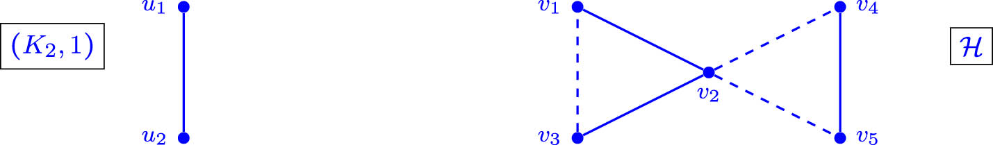
[27, Theorem 5.1] Let ( C n , γ ) be a (directed) T -gain cycle whose gain is e i α . Then,

(2.1) Sp ( C n , γ ) = 2 cos α + 2 π j n ∣ 0 ⩽ j ⩽ n − 1 .

Example 2.2

Let K 3 ( z ) = ( K 3 , γ 3 , z ) and K 3 ′ ( z ) = ( K 3 , γ 3 , z ′ ) be the T -gain graphs depicted in Figure 1. The gains of the directed cycles u 1 u 2 u 3 and v 1 v 2 v 3 in Figure 1 are

γ 3 , z ( u 1 u 2 ) γ 3 , z ( u 2 u 3 ) γ 3 , z ( u 3 u 1 ) = z 2 ⋅ z * = z and γ 3 , z ′ ( v 1 v 2 ) γ 3 , z ′ ( v 2 v 3 ) γ 3 , z ′ ( v 3 v 1 ) = z 3

respectively. If z = e i θ , by Proposition 2.1, we obtain

(2.2) Sp ( K 3 ( z ) ) = 2 cos θ 3 , 2 cos θ + 2 π i 3 , 2 cos θ + 4 π i 3

and

(2.3) Sp ( K 3 ′ ( z ) ) = 2 cos θ , 2 cos θ + 2 π i 3 , 2 cos θ + 4 π i 3 .

The spectra (2.2) and (2.3) can also be obtained by directly computing the characteristic polynomials of the matrices

(2.4) A ( K 3 ( z ) ) = 0 z z z * 0 z z * z * 0 and A ( K 3 ′ ( z ) ) = 0 z z * z * 0 z z z * 0 , .

It turns out that

p K 3 ( z ) ( λ ) = λ 3 − 3 λ − 2 cos θ and p K 3 ′ ( z ) ( λ ) = λ 3 − 3 λ − 2 cos ( 3 θ ) .

It is easily seen that the gain diamond D ( z ) in Figure 1 has two imaginary triangles and a neutral quadrangle. More precisely, the directed cycles C 3 ′ = w 1 w 2 w 3 , C 3 ″ = w 1 w 3 w 4 have both gain e i π 2 = i . It is somehow instructive to see that

(2.5) A ( D ( z ) ) = 0 z i − z * z * 0 − z * 0 − i − z 0 z * − z 0 z 0 and p D(z) ( λ ) = λ 4 − 5 λ 2 ∀ z ∈ T .

Thus, Sp ( D ( z ) ) = { − 5 , 0 ( 2 ) , 5 } , where the exponent of 0 in parentheses stands for its multiplicity.

If Λ = ( H , ζ ) is an induced ( T -gain) subgraph of Γ , i.e., if H is an induced subgraph of G and ζ = γ ∣ E → H , then A ( Λ ) is the principal matrix of A ( Γ ) correspondent to the rows indexed by vertices in V H . Therefore, [22, Corollary 4.3.37] yields the well-known interlacing phenomenon recalled in the following proposition.

Proposition 2.3

Let Λ = ( H , ζ ) be an induced subgraph of Γ = ( G , γ ) with ∣ V G ∣ = n and ∣ V H ∣ = m . Denoted by λ 1 ⩾ λ 2 ⩾ ⋯ ⩾ λ n and μ 1 ⩾ μ 2 ⩾ ⋯ ⩾ μ m the eigenvalues of Γ and Λ , respectively, the following inequalities hold: λ n − m + i ⩽ μ i ⩽ λ i for 1 ⩽ i ⩽ m .

Corollary 2.4

If Γ = ( G , γ ) is a nonempty T -gain graph, then λ 1 ( Γ ) ⩾ 1 .

Proof

Let u and v be two adjacent vertices in G , and let H ≔ G [ u , v ] be the subgraph of G induced by u and v . The index of Λ ≔ ( H , γ ∣ E → H ) is equal to 1; in fact,

(2.6) A ( Λ ) = 0 γ ( u v ) γ ( u v ) * 0 and p Λ ( λ ) = λ 2 − 1 .

Proposition 2.3 now yields λ 1 ( Γ ) ⩾ λ 1 ( Λ ) = 1 .□

Expert scholars know very well that, whatever gain function is chosen on the arcs of a tree, one always retrieves the spectrum of the unsigned tree. This phenomenon occurs whenever the T -gain graph Γ = ( G , γ ) is balanced, since in this case Γ is switching equivalent to ( G , 1 ) . Similarly, the lack of dependence on z for the coefficients of p D(z) in (2.5) is not surprising, as the various graphs in the set { D ( z ) ∣ z ∈ T } are all switching equivalent.

For the notions of balance and switching equivalence, the reader is referred to [10,12,27]. In spite of their significance in the theory of gain graphs, these notions will never be mentioned again in the remainder of this article.

2.2 NEPS and lexicographic products of T -gain graphs

In [9], Belardo et al. introduced NEPS of complex unit gain graphs. In order to keep the article reasonably self-contained, the definition of NEPS will be recalled here.

Let B be a nonempty subset of F h ≔ { 0 , 1 } h \ { ( 0 , … , 0 ) } , the set of { 0 , 1 } - h -tuples with at least one among their components. Cvektović defined G ≔ NEPS ( G 1 , … , G h ; B ) , the non-complete extended p-sums (or simply NEPS) of the simple graphs G 1 , … , G h with basis B (see, for instance, [14, p. 66]): the vertex set V G is the Cartesian product V G 1 × ⋯ × V G h , and the vertices u ≔ ( u 1 , … , u h ) and v ≔ ( v 1 , … , v h ) are adjacent if and only if there exists a (unique) h -tuple b = ( b 1 , … , b h ) in B such that u i = v i whenever b i = 0 , and u i ∼ v i in G i if b i = 1 . Note that

(2.7) E → G = ⨆ b ∈ B E → NEPS ( G 1 , … , G h ; b ) ,

where the symbol ⨆ denotes the disjoint union.

Definition 2.5

Let Γ 1 = ( G 1 , γ 1 ) , … , Γ h = ( G h , γ h ) be h T -gain graphs. The NEPS (or Cvektović product) of Γ 1 , … , Γ h with basis B are the T -gain graph Γ = ( G , γ ) defined as follows:

the underlying graph G is NEPS ( G 1 , … , G h ; B ) ,
for each pair of adjacent vertices u ≔ ( u 1 , … , u h ) and v ≔ ( v 1 , … , v h ) in G ,
(2.8) γ ( u v ) ≔ ∏ j = 1 h γ j ( u j v j ) ,
where γ j ( u j v j ) is understood to be 1 whenever u j = v j .

The T -gain graph Γ = ( G , γ ) will be denoted by NEPS ( Γ 1 , … , Γ h ; B ) .

The map γ in (2.8) is indeed a gain function. In fact,

γ ( v u ) = ∏ j = 1 h γ j ( v j u j ) = ∏ j = 1 h γ j ( u j v j ) * = γ ( u v ) * .

For 1 ⩽ p ⩽ h , let B h , p be the subset of F h of all h -tuples containing precisely p 1’s, and let j h ∈ F h be the all-ones h -tuple ( 1 , … , 1 ) . Clearly, B h , h = { j h } . The T -gain graph NEPS ( Γ 1 , … , Γ h ; B h , p ) is called the (complete) p-sum of Γ 1 , … , Γ h , and

□ i = 1 h Γ i ≔ NEPS ( Γ 1 , … , Γ h ; B h , 1 ) , × i = 1 h Γ i ≔ NEPS ( Γ 1 , … , Γ h ; { j h } ) , ⊠ i = 1 h Γ i ≔ NEPS ( Γ 1 , … , Γ h ; F h )

are the Cartesian product, the direct or tensor product, and the strong product, respectively.

In order to describe how the adjacency matrix of an NEPS is related to those of its factors, we need to recall that, given two matrices B = ( b i j ) and C = ( c i j ) of type k × m and l × n , respectively, the Kronecker product B ⊗ C is the following k l × m n matrix:

B ⊗ C ≔ b 11 C b 12 C ⋯ ⋯ b 1 m C b 21 C b 22 C ⋯ ⋯ b 2 m C ⋮ ⋮ ⋱ ⋱ ⋮ ⋮ ⋮ ⋱ ⋱ ⋮ b k 1 C b k 2 C ⋯ ⋯ b k m C .

Let A be an n × n matrix. In the following statement, A 0 stands for the n × n identity matrix I n .

Proposition 2.6

[9, Proposition 3.3] For 1 ⩽ i ⩽ h , let Γ i be a T -gain graph with n i vertices. The adjacency matrix of Γ = NEPS ( Γ 1 , … , Γ h ; B ) is given by

(2.9) A ( Γ ) = ∑ ( b 1 , … , b h ) ∈ B A ( Γ 1 ) b 1 ⊗ ⋯ ⊗ A ( Γ h ) b h .

Moreover, if λ i 1 ⩾ λ i 2 ⩾ ⋯ ⩾ λ i n i are the eigenvalues of A ( Γ i ) , then Sp ( Γ ) = { λ k 1 , … , k h ∣ 1 ⩽ k i ⩽ n i } , where

(2.10) λ k 1 , … , k h ≔ ∑ ( b 1 , … , b h ) ∈ B λ 1 k 1 b 1 ⋯ λ h k h b h .

The following corollary is extracted from [9, Equation (3.6) and Corollary 3.4].

Corollary 2.7

Let n i be the order of the T -gain graph Γ i for 1 ⩽ i ⩽ h . The adjacency matrix of the Cartesian product □ i = 1 h Γ i is

(2.11) A ( □ i = 1 h Γ i ) = A ( Γ 1 ) ⊗ I n 2 ⊗ ⋯ ⊗ I n h + I n 1 ⊗ A ( Γ 2 ) ⊗ ⋯ ⊗ I n h + ⋯ + I n 1 ⊗ I n 2 ⊗ ⋯ ⊗ A ( Γ h ) .

The spectrum of □ i = 1 h Γ i is

Sp ( □ i = 1 h Γ i ) = { λ 1 k 1 + ⋯ + λ h k h ∣ 1 ⩽ k i ⩽ n i } ,

where λ i 1 ⩾ λ i 2 ⩾ ⋯ ⩾ λ i n i are the eigenvalues of A ( Γ i ) .

In [19], Harary introduced the notion of composition of (simple) graphs later known also as lexicographic product [17, ch. I,4]. In the literature, there are two different extensions to signed graphs of Harary’s composition. The first attempt was made by Hameed and Germina [18], the second is due to Brunetti et al. [11]. In [3], they are respectively called the HG- and the BCD-lexicographic product. We now generalize these two products to T -gain graphs, employing a notation tendentially consistent with [3].

Let G and H be two (unsigned) graphs. The composition or lexicographic product G [ H ] is a graph whose set of vertices is V ( G ) × V ( H ) , with ( u , v ) ∼ ( u ′ , v ′ ) whenever u ∼ u ′ or u = u ′ and v ∼ v ′ .

Definition 2.8

Let Γ = ( G , γ ) and Λ = ( H , ζ ) be two T -gain graphs. The maps

γ HG : ( ( u , v ) ( u ′ , v ′ ) ) ∈ E → G [ H ] ⟼ γ ( u u ′ ) if u ∼ u ′ , ζ ( v v ′ ) if u = u ′ and v ∼ v ′ ,

and

γ BCD : ( ( u , v ) ( u ′ , v ′ ) ) ∈ E → G [ H ] ⟼ γ ( u , u ′ ) if u ∼ u ′ and v ≁ v ′ , γ ( u u ′ ) ζ ( v v ′ ) if u ∼ u ′ and v ∼ v ′ , ζ ( v v ′ ) if u = u ′ and v ∼ v ′ ,

give rise to the following T -gain graphs with underlying graph G [ H ] : the HG-lexicographic product Γ [ Λ ] = ( G [ H ] , γ HG ) and the BCD-lexicographic product Γ ∗ Λ = ( G [ H ] , γ BCD ) .

The reader will easily realize that Definition 2.8 is well-posed: the equalities

γ HG ( ( u , v ) ( u ′ , v ′ ) ) = γ HG ( ( u ′ , v ′ ) ( u , v ) ) * and γ BCD ( ( u , v ) ( u ′ , v ′ ) ) = γ BCD ( ( u ′ , v ′ ) ( u , v ) ) *

are elementary to check; they show that γ HG and γ BCD are both gain functions. The HG-lexicographic product and the BCD-lexicographic product can be iterated. By inductively defining Γ k [ Λ ] ≔ Γ [ Γ k − 1 [ H ] ] and ( ∗ k Γ ) ∗ Λ ≔ ( ∗ k − 1 Γ ) ∗ ( Γ ∗ Λ ) for all k ⩾ 2 , one obtains T -gain graphs whose underlying graph is G k [ H ] , the iterated lexicographic product of simple graphs spectrally investigated by Abreu et al. [1].

The following proposition, whose proof just comes from the definition of the HG-lexicographic product, is the T -gain analog of [18, Theorem 8]. In its statement, J m denotes the m × m all-ones matrix.

Proposition 2.9

Let Γ = ( G , γ ) and Λ = ( H , ζ ) be two T -gain graphs with V G = { u 1 , … , u n } and V H = { v 1 , … , v m } . Chosen for V G × H the lexicographic ordering, the following equality holds:

(2.12) A ( Γ [ Λ ] ) = A ( Γ ) ⊗ J m + I n ⊗ A ( Λ ) .

3 Spectrum of a useful matrix

Let n ⩾ 1 and let u 1 , u 2 , … , u n be the vertices of the complete simple graph K n . In this section, for every z ∈ T , we compute the characteristic polynomial and spectrum of the T -gain graph K n ( z ) = ( K n , γ n , z ) , where γ 1 , z is the empty gain function and, for n ⩾ 2 ,

γ n , z ( u i u j ) = z whenever i < j .

To lighten the notation, we set A n , z ≔ A ( K n ( z ) ) and p n , z ( λ ) ≔ p K n ( z ) ( λ ) = det ( λ I − A n , z ) . By definition,

(3.1) A n , z = 0 z z z … z z * 0 z z … z z * z * 0 z … z z * z * z * 0 … z ⋮ ⋮ ⋮ ⋮ ⋱ ⋮ z * z * z * z * … 0 .

Remark 3.1

The matrix A ( K n ( 1 ) ) is the adjacency matrix of the complex graph K n , whose spectrum is { ( − 1 ) ( n − 1 ) , n − 1 } (see, for instance, [14, p. 72]). Since A ( K n ( − 1 ) ) = − A ( K n ( 1 ) ) , we immediately obtain Sp ( K n ( − 1 ) ) = { 1 ( n − 1 ) , − ( n − 1 ) } . The determinant of an adjacency matrix is the product of its eigenvalues; therefore, det ( A n , 1 ) = ( − 1 ) n − 1 ( n − 1 ) and det ( A n , − 1 ) = − ( n − 1 ) .

Lemma 3.2

For n ⩾ 1 and z = e i θ , the following equality holds:

(3.2) det ( A n , z ) = ( − 1 ) n − 1 ( n − 1 ) for θ = 0 ( i.e. z = 1 ) , − ( n − 1 ) for θ = π ( i.e. z = − 1 ) , ( − 1 ) n − 1 sin ( ( n − 1 ) θ ) sin θ for 0 < θ < π .

Proof

The cases θ ∈ { 0 , π } are dealt in Remark 3.1. From now on, we assume 0 < θ < π . Clearly,

(3.3) det ( A 1 , z ) = 0 and det ( A 2 , z ) = − 1 for all z ∈ T .

Thus, (3.2) holds for n = 2 . Let now n ⩾ 3 . By subtracting the second row to the first one, and the second column to the first one afterwards, one obtains

det ( A n , z ) = det − 2 cos θ z 0 0 … 0 z * 0 z z … z 0 z * 0 z … z 0 z * z * 0 … z ⋮ ⋮ ⋮ ⋮ ⋮ 0 z * z * z * … 0 .

In fact, z + z * = 2 cos θ . Cofactor expansion along the first row gives

det ( A n , z ) = − 2 cos θ det ( A n − 1 , z ) − z det z * z z … z 0 0 z … z 0 z * 0 … z ⋮ ⋮ ⋮ ⋮ 0 z * z * … 0 = − 2 cos θ det ( A n − 1 . z ) − det ( A n − 2 . z )

or equivalently

(3.4) det ( A n , z ) = − ( z + z * ) det ( A n − 1 , z ) − det ( A n − 2 , z ) .

For 0 < θ < π , the complex number z − z * is nonzero. The recursive formula (3.4) can be solved by taking into account (3.3), arriving at the formula

(3.5) det ( A n , z ) = ( − 1 ) n − 1 z n − 1 − z ¯ n − 1 z − z ¯ = ( − 1 ) n − 1 sin ( ( n − 1 ) θ ) sin θ ,

which, a posteriori, can also be proved from (3.3) and (3.4) by an inductive argument.□

Proposition 3.3

Let n ⩾ 2 and z = e i θ . The characteristic polynomial p n , z ( λ ) = det ( λ I − A n , z ) has the following form:

(3.6) p n , z ( λ ) = ( λ − n + 1 ) ( λ + 1 ) n − 1 for θ = 0 ( i.e. z = 1 ) , ( λ + n − 1 ) ( λ − 1 ) n − 1 for θ = π ( i.e. z = − 1 ) , λ n − ∑ k = 1 n n k sin ( ( k − 1 ) θ ) sin θ λ n − k for 0 < θ < π .

Proof

When θ belongs to { 0 , π } , the expression of p n , z ( λ ) in (3.6) is immediately retrieved from the known spectra Sp ( K n ) = { ( − 1 ) ( n − 1 ) , n − 1 } and Sp ( − ( K n , 1 ) ) = { 1 ( n − 1 ) , − ( n − 1 ) } . Let now 0 < θ < π . Note that p 1 , z ( λ ) = λ and p 2 , z ( λ ) = λ 2 − 1 , consistently with (3.6).

Let now n ⩾ 3 . The coefficient of λ n − k in p n , z ( λ ) is given by ( − 1 ) k times the sum of all principal k × k minors of the matrix A n , z . They are all equal to det ( A k , z ) and there are n k of them. Now, equation (3.5) yields

(3.7) p n , z ( λ ) = λ n + ∑ k = 1 n n k ( − 1 ) k det ( A k , z ) λ n − k = λ n + ∑ k = 1 n n k ( − 1 ) k ( − 1 ) k − 1 sin ( ( k − 1 ) θ ) sin θ λ n − k = λ n − ∑ k = 1 n n k sin ( ( k − 1 ) θ ) sin θ λ n − k

as wanted.□

The proof of the next result employs the prosthaphaeresis formulas:

(3.8) cos a − cos b = − 2 sin a + b 2 sin a − b 2

and

(3.9) sin a sin b = cos ( a − b ) − cos ( a + b ) 2 .

Proposition 3.4

Let z = e i θ with 0 < θ < π . The roots of p n , z ( λ ) , i.e., the eigenvalues of the matrix (3.2), are given by the numbers

(3.10) f n , k ( θ ) = sin ( n − 1 ) θ − k π n sin θ + k π n for 0 ⩽ k ⩽ n − 1 .

Moreover,

(3.11) f n , 0 ( θ ) > f n , 1 ( θ ) > ⋯ > f n , n − 1 ( θ ) .

Proof

Let T n = { e 2 h π i n ∣ 0 ⩽ h ⩽ n − 1 } denote the set of the n -th roots of unity. In our hypotheses, z − z * is nonzero and, from (3.5) and (3.6), it follows that

p n , z ( λ ) = λ n − ∑ k = 1 n n k z k − 1 − z ¯ k − 1 z − z ¯ λ n − k = z ( λ + z * ) n − z * ( λ + z ) n z − z * .

Therefore, p n , z ( λ ) = 0 if and only if

(3.12) z * ( λ + z ) n = z ( λ + z * ) n .

By extracting the n -th root, (3.12) is equivalent to

(3.13) ξ * ( λ + z ) = q ξ ( λ + z * ) for ξ ≔ e i θ n and some q ∈ T n .

Observe that the complex number q ξ − ξ 2 is nonzero for all q ∈ T n ; in fact, by setting q = e 2 k π i n and α ≔ ( θ + k π ) ∕ n ,

(3.14) ∣ q ξ − ξ 2 ∣ 2 = ( q ξ − ξ 2 ) ( q * ξ * − ( ξ * ) 2 ) = 2 ( 1 − Re ( q ξ 2 ) ) = 2 ( 1 − cos ( 2 α ) ) = 4 sin 2 α ,

which is nonzero, since

0 < θ n ⩽ α ⩽ θ + ( n − 1 ) π n < π .

Hence, all the roots of (3.12) can be obtained by collecting the values of λ satisfying (3.13); namely,

ξ n − 1 − q ( ξ * ) n − 1 q ξ − ξ * = ξ n − 1 − q ( ξ * ) n − 1 ∣ q ξ − ξ * ∣ 2 ⋅ ( q * ξ * − ξ ) = 2 Re ( q * ξ n − 2 ) − Re ( ξ n ) ∣ q ξ − ξ * ∣ 2 for q ∈ T n .

From (3.14) and the equalities

Re ( q * ξ n − 2 ) = cos ( n − 2 ) θ − 2 k π n and Re ( ξ n ) = Re ( z ) = cos ( θ ) ,

one sees that the roots of p n , z ( λ ) are

(3.15) f n , k ( θ ) = cos ( n − 2 ) θ − 2 k π n − cos ( θ ) 2 sin 2 θ + k π n for 0 ⩽ k ⩽ n − 1 ,

and we arrive at (3.10) by replacing the numerator of (3.15) according to formula (3.8).

The remainder of the proof consists in a suitable sequence of “if and only if” steps. Let f n , k 1 ( θ ) and f n , k 2 ( θ ) be two eigenvalues of A n , z . The first, the second, and the fourth of the following steps are, respectively, due to the positivity of all the denominators in (3.10), (3.9), and (3.8).

f n , k 1 ( θ ) > f n , k 2 ( θ ) ⇔ sin ( n − 1 ) θ − k 1 π n sin θ + k 2 π n > sin ( n − 1 ) θ − k 2 π n sin θ + k 1 π n ⇔ cos ( n − 2 ) θ − ( k 1 + k 2 ) π n − cos θ + k 2 − k 1 n > cos ( n − 2 ) θ − ( k 1 + k 2 ) π n − cos θ + ( k 1 − k 2 ) π n , ⇔ cos θ − ( k 2 − k 1 ) π n − cos θ + ( k 2 − k 1 ) π n > 0 , ⇔ 2 sin θ sin ( k 2 − k 1 ) π n > 0 .

The latter is true if and only if k 2 > k 1 , proving the sequence of inequalities (3.11) and ending the proof.□

The trigonometric identity recalled in the following lemma concerns the collection of real functions { D m ( x ) } m ⩾ 0 known as the Dirichlet kernel (one of the existing proofs can be found, for instance, in [4, p. 175]).

Lemma 3.5

Let m be any nonnegative integer. The following equality holds:

D m ( x ) ≔ 1 + 2 ∑ h = 1 m cos ( h x ) = sin m + 1 2 x sin x 2 ,

for every x ∉ { 2 k π ∣ k ∈ Z } .

Proposition 3.6

For all n ⩾ 3 , the map Ψ n : θ ∈ [ 0 , π ] ⟼ λ 1 ( K n ( e i θ ) ) ∈ R is continuous and strictly decreasing. The image of Ψ n is the interval [ 1 , n − 1 ] .

Proof

The maps Ψ 1 and Ψ 2 are constant. In fact, Ψ 1 ( θ ) = 0 and Ψ 2 ( θ ) = 1 for every θ ∈ [ 0 , 1 ] . Let now n ⩾ 3 and let f n , 0 : ( 0 , π ) ⟶ R be one of the functions considered in (3.10). Since

lim θ → 0 f n , 0 ( θ ) = n − 1 and lim θ → π f n , 0 ( θ ) = 1 ,

the map

f ˜ n , 0 : θ ∈ [ 0 , π ] ⟼ n − 1 if θ = 0 , f n , 0 ( θ ) if 0 < θ < π , 1 if θ = π ,

is continuous in its entire domain and, by Remark 3.1 and Proposition 3.4, it turns out that Ψ n ( θ ) = f ˜ n , 0 ( θ ) for all θ ∈ [ 0 , 1 ] . In order to see that Ψ n is strictly decreasing, a different argument is needed according to the parity of n .

Case 1: n is even. Let n = 2 k with k ⩾ 2 . The number Ψ n ( θ ) = f ˜ n , 0 ( θ ) can be expressed in terms of a suitable Dirichlet kernel (see Lemma 3.5). More precisely,

(3.16) Ψ n ( θ ) = f ˜ n , 0 ( θ ) = D k − 1 ( 2 θ ∕ n ) = 1 + 2 ∑ h = 1 k − 1 cos h θ k .

Thus, Ψ 2 k ( θ ) is strictly decreasing since it is sum of functions which are strictly decreasing in the interval [ 0 , π ] ; namely,

1 + 2 cos θ k , 2 cos 2 θ k , … , 2 cos ( k − 1 ) θ k .

Case 2: n is odd. Let n = 2 k + 1 with k ⩾ 1 . The addition formula for the sine gives

(3.17) f 2 k + 1 , 0 ( θ ) = sin ( n − 2 ) θ n + θ n sin θ n = f n − 1 ( θ ) cos θ n + cos ( n − 2 ) θ n for 0 < θ < π .

Since f n − 1 ( θ ) = f 2 k ( θ ) is constant for k = 1 and it is strictly decreasing in ( 0 , π ) for k > 1 by Case 1, the function f 2 k + 1 , 0 ( θ ) is also strictly decreasing in ( 0 , π ) , being the sum of two strictly decreasing functions; namely, f n − 1 , 0 ( θ ) cos ( θ ∕ n ) and cos ( ( n − 2 ) θ ∕ n ) . The already proved continuity of Ψ n in the closed interval [ 0 , π ] ends the proof.□

Proof of Theorem 1.1

Let Ω ( a ) be the class of all connected T -gain graphs Γ such that λ 1 ( Γ ) = a . The set Ω ( 0 ) is a singleton; in fact, it only contains K 1 equipped with the empty gain function. Moreover, Ω ( a ) = ∅ for all a ∈ ( 0 , 1 ) by Corollary 2.4. Along the proof of that corollary it has also been observed that the T -gain graphs K 2 ( z ) are in Ω ( 1 ) for all z ∈ T .

Let now a > 1 . Since the number ⌈ a ⌉ + 1 is at least 3, Proposition 3.6 ensures that an inverse function Ψ n − 1 : [ 1 , n − 1 ] ⟶ [ 0 , π ] of Ψ n exists for n ⩾ ⌈ a ⌉ + 1 ⩾ 3 . Let θ n ≔ Ψ n − 1 ( a ) . The inclusion

(3.18) { K n ( e i θ n ) ∣ n ⩾ ⌈ a ⌉ + 1 } ⊆ Ω ( a ) .

proves both Parts (i) and (ii) of Theorem 1.1.

Part (iii) also comes from (3.18) and the fact that Ω ( a ) does not contain T -gain graphs with less than ⌈ a ⌉ + 1 vertices. In order to see this, let Δ G denote the maximum vertex degree of a graph G with ∣ V G ∣ ⩽ ⌈ a ⌉ . Clearly Δ G ⩽ ∣ V G ∣ − 1 ⩽ ⌈ a ⌉ − 1 and, as a consequence of [27, Theorem 4.3], the index of Γ = ( G , γ ) cannot be larger than Δ G ⩽ ⌈ a ⌉ − 1 < a .□

Remark 3.7

Theorem 1.1 admits a shorter but more conceptual proof, for which Propositions 3.3, 3.4, and 3.6 are not really needed: since the entries of the Hermitian matrix A n , e i θ continuously depend on θ , the eigenvalues

λ 1 ( A n , e i θ ) ⩾ ⋯ ⩾ λ n ( A n , e i θ )

are continuous functions with respect to θ . This is quite a well-known fact in perturbation theory sometimes referred as “the Rellich’s theorem.” In fact, a proof can be found in [28, p. 39]. It follows that the image of the map

Ψ n : θ ∈ [ 0 , π ] ⟼ λ 1 ( A n , e i θ ) ∈ R

is a connected subset of R . Since 1 = λ 1 ( A n , − 1 ) and n − 1 = λ 1 ( A n , 1 ) are both in Θ , then [ 1 , n − 1 ] ⊆ Im ( Ψ n ) . In spite of its elegance and shortness, this approach does not allow one to detect, for any fixed a ∈ R , which (and how many) z ’s make K n ( z ) belonging to Ω ( a ) .

Corollary 3.8

For every real number c ∈ R , there exists a T -gain graph Γ = ( G , γ ) such that c belongs to Sp ( Γ ) .

Proof

If c belongs to Sp ( Γ ) , then − c belongs to Sp ( − Γ ) . Thus, it is not restrictive to assume c ⩾ 0 . For c ∈ { 0 } ∪ [ 1 , + ∞ ) , the result immediately follows from Theorem 1.1. If instead c ∈ ( 0 , 1 ) , then c ∈ Sp ( K 3 ′ ( e i θ ) ) for θ = arccos ( c ∕ 2 ) by (2.3) (the graph K 3 ′ ( e i θ ) is depicted in Figure 1).□

4 a - T -regularity and products

In Section 1, a - T -regular graphs have been defined, and it has also been observed that a - T -regular graphs with n vertices are precisely the T -gain graphs having the all-ones vector j n in their spectrum. However, it should be noted that, contrarily to what happens for simple graphs as a consequence of the Perron-Froebenius theorem, the number a is not necessarily the largest eigenvalue of a - T -regular graphs. For instance, the graph K 3 ′ ( e i θ ) considered in Example 2.2 is 2 cos θ -regular; yet, 2 cos θ is not the largest eigenvalue for π ∕ 3 < θ ⩽ π . The next proposition shows how a - T -regularity behaves with respect to the several products recalled in Section 2.

Proposition 4.1

For 1 ⩽ i ⩽ h , let Γ i be an a i - T -regular graph with n i vertices, and let B be a nonempty subset of F h ≔ { 0 , 1 } h \ { ( 0 , … , 0 ) } .

The T -gain graph Γ = NEPS ( Γ 1 , … , Γ h ; B ) is r - T -regular for
r = ∑ ( b 1 , … , b h ) ∈ B a 1 b 1 ⋯ a h b h .
The HG-lexicographic product Γ 1 [ Γ 2 ] is s - T -regular for s = a 1 n 2 + a 2 .

Proof

The T -gain graph Γ has n ≔ ∏ i = 1 h n i vertices. Using Proposition 2.6 and the properties of the tensor product of matrices,

A ( Γ ) j n = ∑ ( b 1 , … , b h ) ∈ B A ( Γ 1 ) b 1 ⊗ ⋯ ⊗ A ( Γ h ) b h ⨂ i = 1 h j n i = ∑ ( b 1 , … , b h ) ∈ B ( A ( Γ 1 ) b 1 j n 1 ) ⊗ ⋯ ⊗ ( A ( Γ 1 ) b h j n h ) = ∑ ( b 1 , … , b h ) ∈ B ( a 1 b 1 j n 1 ) ⊗ ⋯ ⊗ ( a h b h j n h ) = ∑ ( b 1 , … , b h ) ∈ B a 1 b 1 ⋯ a h b h j n 1 ⊗ ⋯ ⊗ j n h = r j n .

This proves Part (i). The proof of Part (ii) relies on (2.9):

□ A ( Γ [ Λ ] ) j n 1 n 2 = ( A ( Γ ) ⊗ J n 2 ) ( j n 1 ⊗ j n 2 ) + ( I n 1 ⊗ A ( Λ ) ) ( j n 1 ⊗ j n 2 ) = ( A ( Γ ) j n 1 ) ⊗ ( J n 2 j n 2 ) + j n 1 ⊗ A ( Λ ) j n 2 = ( a 1 j n 1 ) ⊗ ( n 2 j n 2 ) + j n 1 ⊗ ( a 2 j n 2 ) = ( a 1 n 2 + a 2 ) j n 1 ⊗ j n 2 = s j n 1 n 2 .

The reader could ask whether the BCD-lexicographic product preserves T -regularity. The answer is negative in general. In Figure 2, the graph Γ ≔ ( K 2 , 1 ) is 1- T -regular, whereas the signed hourglass Λ ≔ ℋ = ( H , ζ ) is 0- T -regular (the gain function ζ is defined as follows: ζ ( v 1 v 2 ) = ζ ( v 2 v 3 ) = ζ ( v 4 v 5 ) = 1 and ζ ( v 1 v 3 ) = ζ ( v 2 v 4 ) = ζ ( v 2 v 5 ) = − 1 ). The submatrix of A ( Γ ∗ Λ ) consisting of the rows indexed by ( u 1 , v 1 ) and ( u 1 , v 2 ) is

B = 0 1 − 1 0 0 1 1 − 1 1 1 1 0 1 − 1 − 1 1 1 1 − 1 − 1 .

By looking at B , one realizes that the T -outgains of the vertices ( u 1 , v 1 ) and ( u 1 , v 2 ) in Γ ∗ Λ are different. More precisely,

d Γ ∗ Λ → ( u 1 , v 1 ) = 3 ≠ 1 = d Γ ∗ Λ → ( u 1 , v 2 ) .

Proposition 4.1 and (2.11) lead without difficulty to the following result.

$Figure 2 ( K 2 , 1 ) \left({K}_{2},1) and the signed hourglass ℋ {\mathcal{ {\mathcal H} }} . Dashed lines represent negative edges.$

Figure 2

( K 2 , 1 ) and the signed hourglass ℋ . Dashed lines represent negative edges.

Corollary 4.2

For 1 ⩽ i ⩽ h , let Γ i be an a i - T -regular graph. The Cartesian product □ i = 1 h Γ i is an a - T -regular graph with a = a 1 + ⋯ + a h .

Proof of Theorem 1.3

For a ∈ R , let ℛ ( a ) be the set of connected a - T -regular graphs, and let v be a vertex of a T -gain graph Γ . Since d − Γ → ( v ) = − d Γ → ( v ) , it will be suffice to show that ℛ ( a ) contains infinitely many T -gain graphs for a ⩾ 0 . In Example 2.2, the 2 Re ( z ) -regular triangle K 3 ′ ( z ) has been introduced. Corollary 4.2 implies

Γ ˜ h ≔ K 3 ′ ( i ) □ ⋯ □ K 3 ′ ( i ) ︸ h times ∈ ℛ ( 0 ) for all h ⩾ 1 ,

proving the statement for a = 0 . For a > 0 , three cases will be considered. In all of them, Corollary 4.2 will be used.

Case 1: a is a positive integer. Since ( K a + 1 , 1 ) is a - T -regular,

{ ( K a + 1 , 1 ) } ∪ { ( K a + 1 , 1 ) □ Γ ˜ h ∣ h ⩾ 1 } ⊆ ℛ ( a ) .

Case 2: 0 < a < 2 . If θ a ≔ arccos ( a ∕ 2 ) , { K 3 ′ ( e i θ a ) } ∪ { K 3 ′ ( e i θ a ) □ Γ ˜ h ∣ h ⩾ 1 } ⊆ ℛ ( a ) .

Case 3: a > 2 . The number p ≔ ( a − ⌊ a ⌋ + 1 ) ∕ 2 belongs to [ 1 ∕ 2 , 1 ) . For ω a ≔ arccos p , the T -gain graph Λ a ≔ ( K ⌊ a ⌋ , 1 ) □ K 3 ′ ( e i ω a ) is a - T -regular; in fact, ⌊ a ⌋ − 1 + 2 cos ω a = ⌊ a ⌋ − 1 + 2 p = a . Therefore,

{ Λ a } ∪ { Λ a □ Γ ˜ h ∣ h ⩾ 1 } ⊆ ℛ ( a ) ,

and the proof is completed.□

In the proof of Theorem 1.3, Case 1 could be absorbed in Cases 2 and 3: if a is a positive integer ( K a + 1 , 1 ) and Λ a ≔ ( K a , 1 ) □ K 3 ′ ( e 1 2 i ) are both a - T -regular, yet the former has a smaller number of vertices. In fact, for a ⩾ 0 , ℛ ( a ) surely contains: a graph of order a + 1 if a is an integer, and a graph of order max { 3 , 3 ⌊ a ⌋ } if a is not an integer. In any case, a suitable join-like construction, when a is not an integer, will lead to the detections of items in ℛ ( a ) with no more than ⌊ a ⌋ + 4 vertices.

Definition 4.3

Let Γ = ( G , γ ) and Γ ′ = ( G ′ , γ ′ ) be two nonempty T -gain graphs with V G = { u 1 , … , u n } and V G ′ = { u 1 ′ , … , u m ′ } , and let G ∨ G ′ denote the usual join between G and G ′ . For z ∈ T , we define a gain function γ z on the set E → G ∨ G ′ as follows:

γ z ( u i u j ) ≔ γ ( u i u j ) , γ z ( u i ′ u j ′ ) ≔ γ ′ ( u i ′ u j ′ ) and γ z ( u i u j ′ ) = γ z ( u j ′ u i ) * = z if i + j is even ; z * if i + j is odd.

The z -join Γ ∨ z Γ ′ is, by definition, the T -gain graph ( G ∨ G ′ , γ z ) .

Chosen for V G ∨ G ′ the ordering u 1 , … , u n , u 1 ′ , … , u m ′ , the adjacency matrix of Γ ∨ z Γ ′ reads as follows:

A ( Γ ∨ z Γ ′ ) = A ( Γ ) z z * … z * z … ⋮ ⋮ ⋱ z * z … z z * … ⋮ ⋮ ⋱ A ( Γ ′ ) .

The following lemma is straightforward.

Lemma 4.4

If Γ and Γ ′ are a - T -regular graphs having the same even number of vertices n, then Γ ∨ z Γ ′ is a b - T -regular graph, with b = a + n Re ( z ) .

The following Theorem 4.5 is the last result of this article.

Theorem 4.5

Let a be any real number. Then, ℛ ( a ) contains at least one T -gain graph whose order is not larger than ∣ a ∣ + 5 .

Proof

If Γ belongs to ℛ ( a ) , then − Γ belongs to ℛ ( − a ) . Thus, it is not restrictive to assume a ⩾ 0 . If 0 ⩽ a ⩽ 2 , the statement surely holds since (as seen in Case 2 of the previous proof) ℛ ( a ) contains a T -gain triangle. Furthermore, the statement is trivially verified when a is a positive integer, since ( K a + 1 , 1 ) ∈ ℛ ( a ) . From now on, a is assumed to be a real number larger than 2 which is not an integer, and h ≔ ⌊ a ∕ 4 ⌋ .

Case 1: ⌊ a ⌋ = 4 h + ε for ε ∈ { 0 , 1 , 2 } . Let z ˜ 1 be a complex unit such that

Re ( z ˜ 1 ) = 2 h + ε − 1 + a − ⌊ a ⌋ 2 h + 2 .

From Lemma 4.4, the T -gain graph ( K 2 h + 2 , 1 ) ∨ z ˜ 1 ( K 2 h + 2 , 1 ) , whose order is ⌊ a ⌋ + 4 − ε < a + 5 , belongs to ℛ ( a ) .

Case 2: ⌊ a ⌋ = 4 h + 3 . Let z ˜ 2 be a complex unit such that

Re ( z ˜ 2 ) = 2 h + a − ⌊ a ⌋ 2 h + 4 .

From Lemma 4.4, the T -gain graph ( K 2 h + 4 , 1 ) ∨ z ˜ 2 ( K 2 h + 4 , 1 ) is a - T -regular. Its order is ⌊ a ⌋ + 5 < a + 5 .□

Acknowledgements

The author is indebted to Francesco D’Andrea for (3.13) and the first equality of (3.5). The author also thanks the anonymous referees for their careful reading and appreciation. This research has been supported by INDAM-GNSAGA.

Author contributions: The author confirms sole responsibility for the following: manuscript preparation; study conception and design; data collection; analysis and interpretation of results.
Conflict of interest: The author states no conflict of interest.
Data availability statement: Data sharing is not applicable to this article as no datasets were generated or analysed during the current study.

References

[1] N. Abreu, D. M. Cardoso, P. Carvalho, and C. T. M. Vinagre, Spectra and Laplacian spectra of arbitrary powers of lexicographic products of graphs, Discrete Math. 340 (2017), no. 1, 3235–3244. 10.1016/j.disc.2016.07.017Suche in Google Scholar

[2] A. Alazemi, F. Belardo, M. Brunetti, M. Andelić, and C. M. da Fonseca, Line and subdivision graphs determined by T4-gain graphs, Mathematics 7 (2019), no. 10, 926. 10.3390/math7100926Suche in Google Scholar

[3] M. Albin and K. A. Germina, Vector valued switching in the products of signed graphs, Commun. Comb. Optim. 9 (2024) 759–771. https://doi.org/10.22049/CCO.2023.28758.1703. Suche in Google Scholar

[4] G. Bachman, L. Narici, and E. Beckenstein, Fourier and Wavelet Analysis, 2nd edition, Springer-Verlag, New York, 2002. Suche in Google Scholar

[5] F. Belardo and M. Brunetti, Line graphs of complex unit gain graphs with least eigenvalue −2, Electron. J. Linear Algebra 37 (2021), 14–30. 10.13001/ela.2021.5249Suche in Google Scholar

[6] F. Belardo and M. Brunetti, On eigenspaces of some compound complex unit gain graphs, Trans. Comb. 11 (2022), no. 3, 131–152. Suche in Google Scholar

[7] F. Belardo, M. Brunetti, and A. Ciampella, Edge perturbation on signed graphs with clusters: Adjacency and Laplacian eigenvalues, Discr. Appl. Math. 269 (2019), 130–138. 10.1016/j.dam.2019.02.018Suche in Google Scholar

[8] F. Belardo, M. Brunetti, M. Cavaleri, and A. Donno, Godsil-McKay switching for mixed and gain graphs over the circle group, Linear Algebra Appl. 614 (2021), 256–269. 10.1016/j.laa.2020.04.025Suche in Google Scholar

[9] F. Belardo, M. Brunetti, and S. Khan, NEPS of complex unit gain graphs, Electron. J. Linear Algebra 39 (2023), 621–643. 10.13001/ela.2023.8015Suche in Google Scholar

[10] F. Belardo, M. Brunetti, and N. Reff, Balancedness and the least Laplacian eigenvalue of some complex unit gain graphs, Discuss. Math. Graph Theory 40 (2020), no. 2, 417–433. 10.7151/dmgt.2281Suche in Google Scholar

[11] M. Brunetti, M. Cavaleri, and A. Donno, A lexicographic product for signed graphs, Australas. J. Combin. 74 (2019), 332–343. Suche in Google Scholar

[12] M. Cavaleri, D. D’Angeli, and A. Donno, A group representation approach to the balance of gain graph. J. Algebr. Comb. 54 (2021), 265–293. 10.1007/s10801-020-00977-wSuche in Google Scholar

[13] M. Cavaleri and A. Donno, On cospectrality of gain graphs, Spec. Matrices 10 (2022), 343–365. 10.1515/spma-2022-0169Suche in Google Scholar

[14] D. M. Cvetković, M. Doob, and H. Sachs, Spectra of Graphs, Theory and Application, 3rd edition, Johann Ambrosius Barth Verlag, Heidelberg-Leipzig, 1995. Suche in Google Scholar

[15] D. R. Estes, Eigenvalues of symmetric integer matrices, J. Number Theory 42 (1992), no. 3, 292–296. 10.1016/0022-314X(92)90094-6Suche in Google Scholar

[16] K. Guo and B. Mohar, Hermitian adjacency matrix of digraphs and mixed graphs, J. Graph Theory 85 (2017), no. 1, 217–248. 10.1002/jgt.22057Suche in Google Scholar

[17] R. Hammack, W. Imrich, and S. Klavžar, Handbook of Product Graphs., 2nd edition, CRC Press, Boca Raton, 2011. 10.1201/b10959Suche in Google Scholar

[18] S. Hameed and K. A. Germina, On Composition of signed graphs, Discuss. Math. Graph Theory 32 (2012), 507–516. 10.7151/dmgt.1615Suche in Google Scholar

[19] F. Harary, On the group of the composition of two graphs, Duke Math. J. 26 (1959), 29–34. 10.1215/S0012-7094-59-02603-1Suche in Google Scholar

[20] S. He, R.-X. Hao, and F. Dong, The rank of a complex unit gain graph in terms of the matching number, Linear Algebra Appl. 589 (2020), 158–185. 10.1016/j.laa.2019.12.014Suche in Google Scholar

[21] A. J. Hoffman, On limit points of spectral radii of non-negative symmetric integral matrices, in: Y. Alavi, et al. (Eds.), Lecture Notes Math, vol. 303, Springer-Verlag, Berlin, 1972, pp. 165–172. 10.1007/BFb0067367Suche in Google Scholar

[22] R. A. Horn and e C. R. Johnson, Matrix Analysis, Cambridge University Press, Cambridge, 2012. Suche in Google Scholar

[23] M. Kannan, N. Kumar, and S. Pragada, Bounds for the extremal eigenvalues of gain Laplacian matrices, Linear Algebra Appl. 625 (2021), 212–240. 10.1016/j.laa.2021.05.009Suche in Google Scholar

[24] D. Lind and B. Marcus, An Introduction to Symbolic Dynamics and Coding, Cambridge University Press, Cambridge, 1995. 10.1017/CBO9780511626302Suche in Google Scholar

[25] L. Lu, J. Wang, and Q. Huang, Complex unit gain graphs with exactly one positive eigenvalue, Linear Algebra Appl. 608 (2021), 270–281. 10.1016/j.laa.2020.09.016Suche in Google Scholar

[26] R. Metahari, M. R. Kannan, and A. Samanta, On the adjacency matrix of a complex unit gain graph, Linear Multilinear Algebra 70 (2022), no. 9, 1798–1813. 10.1080/03081087.2020.1776672Suche in Google Scholar

[27] N. Reff, Spectral properties of complex unit gain graphs, Linear Algebra Appl. 436 (2012), no. 9, 3165–3176. 10.1016/j.laa.2011.10.021Suche in Google Scholar

[28] F. Rellich, Perturbation Theory of Eigenvalue Problems, Gordon and Breach, New York, 1969. Suche in Google Scholar

[29] P. Rowlinson and Z. Stanić, Signed graphs with three eigenvalues: Biregularity and beyond, Linear Algebra Appl. 621 (2021)272–295. 10.1016/j.laa.2021.03.018Suche in Google Scholar

[30] J. Salez, Every totally real algebraic integer is a tree eigenvalue, J. Comb. Theory B 111 (2015), 249–256. 10.1016/j.jctb.2014.09.001Suche in Google Scholar

[31] A. Samanta and M. R. Kannan, Gain distance matrices for complex unit gain graphs, Discrete Math. 345 (2022), no. 1, 112634. 10.1016/j.disc.2021.112634Suche in Google Scholar

[32] Z. Stanić, On strongly regular signed graphs, Discr. Appl. Math. 271 (2019), 184–190. 10.1016/j.dam.2019.06.017Suche in Google Scholar

[33] Z. Stanić, Some relations between the largest eigenvalue and the frustration index of a signed graph, Am. J. Comb. 1 (2022), 65–72. Suche in Google Scholar

[34] Y. Wang, S.-C. Gong, and Y.-Z. Fan, On the determinant of the Laplacian matrix of a complex unit gain graph, Discrete Math. 341 (2018), no. 1, 81–86. 10.1016/j.disc.2017.07.003Suche in Google Scholar

[35] P. Wissing and E. van Dam, Unit gain graphs with two distinct eigenvalues and systems of lines in complex space, Discrete Math. 345 (2022), Art. 112827. 10.1016/j.disc.2022.112827Suche in Google Scholar

Received: 2024-02-13

Revised: 2024-04-09

Accepted: 2024-04-10

Published Online: 2024-05-16

This work is licensed under the Creative Commons Attribution 4.0 International License.

Artikel in diesem Heft

https://doi.org/10.1515/spma-2024-0005

Schlagwörter für diesen Artikel

gain graph; eigenvalues; index; T-regularity

Creative Commons

BY 4.0