Eigenpairs of adjacency matrices of balanced signed graphs

Mei-Qin Chen

doi:10.1515/spma-2024-0007

Article Open Access

Eigenpairs of adjacency matrices of balanced signed graphs

Mei-Qin Chen

Published/Copyright: July 10, 2024

Published by

Become an author with De Gruyter Brill

Submit Manuscript Author Information Explore this Subject

From the journal Special Matrices Volume 12 Issue 1

Abstract

In this article, we study eigenvalues λ and their associated eigenvectors x of the adjacency matrices A of balanced signed graphs. Balanced signed graphs were first introduced and studied by Harary to handle a problem in social psychology. Harary showed in 1953 that a signed graph is balanced if and only if its vertex set V can be divided into two sets (either of which may be empty), X and Y , so that each edge between the sets is negative and each within a set is positive. Based on this fundamental theorem for the balanced signed graphs, vertices of a balanced signed graph can be labeled in a way so that its adjacency matrix is well structured. Using this special structure, we find algebraically all eigenvalues and their associated eigenvectors of the adjacency matrix A of a given balanced signed graph. We present in this study eigenpairs ( λ , x ) of adjacency matrices of balanced signed graphs with some special structures.

Keywords: balanced signed graphs; structured adjacency matrix of a signed graph; eigenvalues and eigenvectors of an adjacency matrix

MSC 2010: 15A18; 65F15; 05C50; 05C22

1 Introduction

In graph theory, a graph G = ( V , E ) is an abstract representation of a set of objects V together with a set of unordered pairs E taken from V . The elements of V are called vertices, and the elements of E are called edges that are links adjoining vertices. Vertices u and v are adjacent if { u , v } (or u v for short) is an edge in E . For example, the triangle graph with vertices { a , b , c } has edges { a b , b c , c a } . In a graph G , an edge that connects a vertex to itself is called a loop, and multiple edges are two or more edges that are incident to the same two vertices. A graph is simple if it has no loops or multiple edges. All graphs in this article are simple. A graph of order n (with n vertices) is complete if the edge set E contains each of the n ( n − 1 ) 2 pairs of edges.

A labeled graph is a graph in which labels are attached to vertices or edges. The system of labeling in this study is a binary labeling of edges using “+” or “−” and graphs with this particular labeling are called signed graphs, and its abbreviation sigraphs is used in some literature [1]. The process of attaching “+” or “−” to the edges is called signing. There are many applications and spectrum properties of signed graphs and weighted signed graphs in the literature: [3,12,14–17,19], just to cite a few.

A path in a graph is an ordered list of vertices and edges of the type v , v u , u , u w , w , … , z t , t . For convenience, usually only the vertices are listed: v , u , w , … , z , t . Intuitively, a path is the directed walk one might take if the graph were geometrically laid out on a surface. A closed path has the same initial and final vertices. A path is simple if it has no repeated interior vertices. A cycle is a simple closed path. A path is positive if the number of negatively signed edges in it is even, and otherwise, the path is negative.

A signed graph is said to be balanced if every cycle is positive. The sign of a cycle is thus the “product” of the signs of its edges, i.e. the product when “+” and “−” are replaced by 1 and − 1 , respectively, and we correspondingly speak of positive or negative cycles. When a balanced signed graph represents a network, it may be called cycle balance [1] or net-balance [18]. Balanced signed graphs were first introduced and studied by Cartwright and Harary [4] and Harary [11], to handle a problem in social psychology. Some examples in psychology can be found in [8,20]. There have been many more applications of balanced signed graphs and further developments in the spectra of graphs in recent literature [2,5,6,7,10,21,22]. In [22], the switching scheme and Seidel Matrix are used to study the spectra of a balanced signed graph. Note that a vertex switching means switching a single vertex and the Seidel Matrix of a graph S = [ s i j ] is defined as s i i = 0 , s i j = 1 if there is an edge between the i th vertex and the j th vertex and s i j = − 1 otherwise. One can also find a detailed survey on graph labelings in [9].

The following theorem given by Harary in 1953 is the first theorem of signed graphs and is fundamental for balanced signed graphs. This theorem is also called Harary’s bipartition theorem later [10].

Theorem 1.1

[11] A signed graph is balanced if and only if its vertex set can be divided into two sets (either of which may be empty), X and Y, so that each edge between the sets is negative and each within a set is positive.

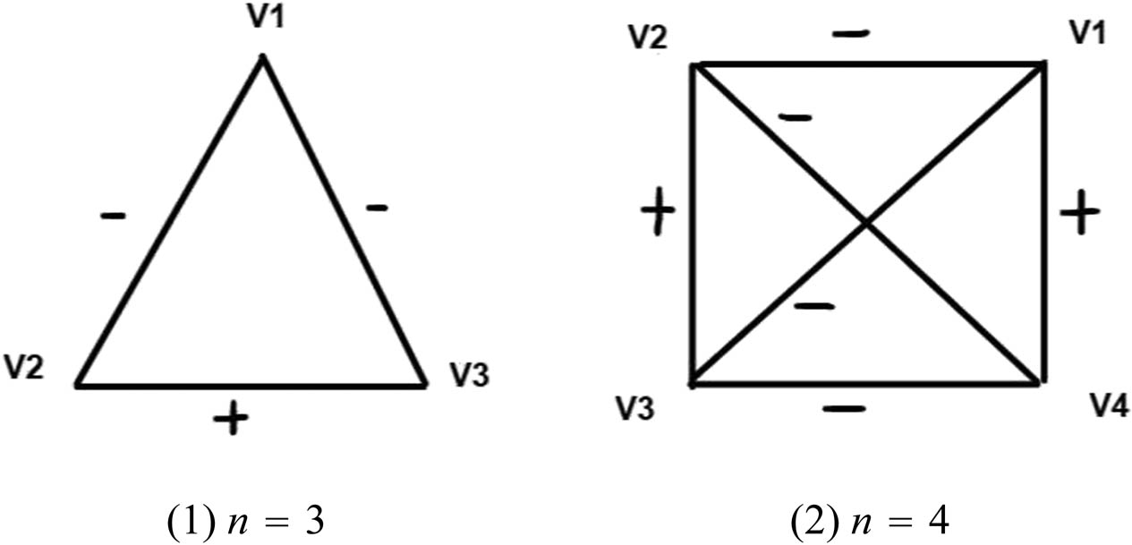
Let { v 1 , … , v n } be n labeled vertices of a signed graph. In Figure 1, two signed graphs with n = 3 and n = 4 , respectively, are balanced, and corresponding sets X and Y in the aforementioned theorem are: X = { v 1 } and Y = { v 2 , v 3 } for n = 3 and X = { v 1 , v 4 } and Y = { v 2 , v 3 } , for n = 4 .

Figure 1

Examples: complete signed graphs.

Let A = [ a i j ] n × n be the n × n adjacency matrix of a signed graph of n vertices. We assign 1 or − 1 to each edge with a positive sign or a negative sign, respectively, and assign 0 if there is no edge between two vertices. By definition, a i i = 0 for all i and a i j = a j i = 1 , − 1 or 0 for all i ≠ j . For the aforementioned two examples, the associated adjacency matrices are

A 1 = 0 − 1 − 1 − 1 0 1 − 1 1 0 and A 2 = 0 − 1 − 1 1 − 1 0 1 − 1 − 1 1 0 − 1 1 − 1 − 1 0 .

Let G be a balanced signed graph with sets of vertices X and Y such that each edge between X and Y is negative and each within X or Y is positive. Let also G X and G Y be subgraphs of G with vertices in X and Y , respectively. With rearranging the vertex set of a balanced signed graph G as { X , Y } , Theorem 1.1 indicates that the adjacency matrix A of G is of the form A = M X N T N M Y , where M X and M Y are adjacency matrices of the subgraphs G X and G Y , respectively, and N is a ( 0 , − 1 ) matrix. The adjacency matrix A 2 for the second example above is not in this form with the order of vertices { v 1 , v 2 , v 3 , v 4 } . However, if the vertices are rearranged as { v 1 , v 4 , v 2 , v 3 } , then the adjacency matrix A 2 = 0 1 − 1 − 1 1 0 − 1 − 1 − 1 − 1 0 1 − 1 − 1 1 0 is in the given form.

Theorem 1.1 can also be used to determine whether or not a given graph with a ( − 1 , 0 , 1 ) adjacency matrix A is balanced. Let P i , j be the elementary matrix for the elementary row operation Type I (interchange the i th and j th rows). Note that P i , j A P i , j is the adjacency matrix of G with switching the vertices v i and v j . Because P i , j A P i , j is similar to A , vertex switching does not change the spectra of a graph by the result (1) in Section 2. The following procedure is developed to determine if a signed graph G is balanced from its adjacency matrix A = [ a i j ] n × n which is a symmetric ( − 1 , 0, 1) matrix with 0’s on its diagonal.

Procedure to determine if a signed graph G is balanced:

Let V = { v 1 , v 2 , … , v n } .

For each row i = 1 , 2 , … , n − 1 , check a i j for j = i + 1 , … , n .

If a i j = − 1 and a i k = 0 or 1 for the first j < k ≤ n , then we switch the j th and k th columns of A and switch the order of v j and v k in V . Continue to check the next row when j = n .

If a i j = − 1 but there is no a i k = 0 or 1 for j < k ≤ n , then the graph G is balanced and X contains the first j vertices in the updated set V if all a i j = − 1 for all i < j ; otherwise, G is not balanced.

Is there another way to check if a given signed graph is balanced? The following two theorems are known as Acharya’s spectra criterion and Stanic’s spectral criterion [1]. Both theorems characterize balanced signed graphs by spectra of graphs.

Theorem 1.2

[1] A signed graph ∑ = ( G , σ ) is balanced if and only if the spectra of the adjacency matrices of ∑ and G coincide.

Theorem 1.3

[10] A signed graph ∑ = ( G , σ ) is balanced if and only if the largest eigenvalues of the adjacency matrices of ∑ and G coincide.

These two theorems can be used to determine if a given signed graph is balanced by checking the spectra of the adjacency matrices of the signed graph ∑ and its underlying graph G .

For this article, we study the eigenvalues of the adjacency matrices of balanced signed completed graphs and their associated eigenvectors, as well as some balanced signed graphs that are not completed but with some special structures. The patterns of the eigenvalues λ and their associated eigenvectors v , in short, eigenpairs ( λ , v ), of adjacency matrices A can also be used to identify some balanced signed graphs. In Section 2, we first review some known properties of eigenpairs of matrices and then study eigenpairs of the adjacency matrices of balanced signed complete graphs K n and balanced signed graphs K n by taking out t edges between vertices in X and Y . We study in Section 3 the eigenpairs of adjacency matrices of balanced complete and incomplete signed bipartite graphs. In Section 4, we further analyze the eigenpairs of adjacency matrices of balanced complete and incomplete signed graphs K n ∘ K t for 2 ≤ t ≤ n . Some properties of balanced signed graphs discussed in this study are known or can be obtained from some results in the graph theory. We present and provide proofs of these properties directly from the special structures and related eigen properties of the adjacency matrices of these graphs. Details will be discussed for each case. Some new results derived through adjacency matrices may also be able to be applied to related results in graph theory.

2 Eigenpairs of adjacency matrices of balanced signed graphs

Let λ be in C , the set of all complex numbers, and x be nonzero in C n , the set of all complex n -column-vectors. Let M be an n × n matrix. If M x = λ x , λ is called an eigenvalue of M with corresponding right eigenvector x , or, ( λ , x ) is called an eigenpair of matrix M . Because an adjacency matrix A is symmetric, it is known that its eigenvalues are real and so are its eigenvectors.

Two n × n matrices M 1 and M 2 are said to be similar, denoted as M 1 ≈ M 2 , if there exists a nonsingular n × n matrix S such that M 2 = S − 1 M 1 S .

The following known results will be used in the study:

[13] Two similar matrices have the same eigenvalues. Let M 1 and M 2 be similar and ( λ , x ) be an eigenpair of M 1 . Because M 1 x = λ x and S − 1 M 1 S S − 1 x = λ S − 1 x , or M 2 ( S − 1 x ) = λ ( S − 1 x ) , ( λ , S − 1 x ) is an eigenpair of M 2 .
[5] Let A n be the adjacency matrix of the complete graph K n with n vertices. Then, A n is a n × n ( 0 , 1 ) matrix with all ones except along the diagonal where there are only zeros. The matrix A n has eigenpairs ( n − 1 , e n ) and ( − 1 , x i ) for i = 1 , 2 , … , n − 1 where e n and x i ’s are n x 1 vectors and
e n = [ 1 , … , 1 ] T , x 1 = [ 1 , − 1 , 0 , … , 0 ] T , x 2 = [ 1 , 0 , − 1 , 0 , … , 0 ] T , … , x n − 1 = [ 1 , 0 , … , 0 , − 1 ] T .

Let A 0 be an adjacency matrix of a balanced signed complete graph G n . Then, A 0 is an n × n ( − 1 , 0 , 1 ) matrix with zeros on its diagonal. By Theorem 1.1, after rearranging vertices { v 1 , v 2 , … , v n } ,

A 0 = A k − E ( n − k ) × k T − E ( n − k ) × k A n − k ,

where A k and A n − k are adjacency matrices of the subgraphs K k and K n − k , respectively, and E is an ( n − k ) × k matrix with all ones. Let S = I k Z ( n − k ) × k T Z ( n − k ) × k − I n − k , where I k and I n − k are k × k and ( n − k ) × ( n − k ) identity matrices, respectively, and Z ( n − k ) × k is an ( n − k ) × k matrix with all zeros. Observe that S A 0 S = A n . Hence, A 0 and A n are similar and A 0 has eigenpairs ( n − 1 , S e n ) and ( − 1 , S x i ) for i = 1 , 2 , … , n − 1 directly from the results (1) and (2) given earlier. We can conclude that for a given adjacency matrix A of a signed complete graph G n , if the eigenvalues of A are not n − 1 and − 1 of multiplicity n − 1 , then G n is not balanced.

What are eigenpairs of the adjacency matrix of a balanced signed graph that is not complete? A signed graph is not complete if there exists at least one pair of vertices that are not adjacent. For a balanced signed graph, vertices that are not adjacent can be in the set X , the set Y , or between sets X and Y . Consider all balanced signed graphs that are derived from the balanced and complete signed graphs with X k and Y k by removing edges among t vertices v n 1 , … v n t , where n j ∈ { 1 , 2 , … , n } and n 1 < ⋯ < n t . For example, two graphs in Figure 2 are obtained from the balanced and complete signed graph of five vertices with X 2 = { v 1 , v 2 } by removing edges between two vertices: (1) v 1 , v 2 and (2) v 1 , v 3 . The associated adjacency matrices C 1 and C 2 are as follows:

C 1 = 0 0 − 1 − 1 − 1 0 0 − 1 − 1 − 1 − 1 − 1 0 1 1 − 1 − 1 1 0 1 − 1 − 1 1 1 0 and C 2 = 0 1 0 − 1 − 1 1 0 − 1 − 1 − 1 0 − 1 0 1 1 − 1 − 1 1 0 1 − 1 − 1 1 1 0 .

Figure 2

Examples: incomplete signed graphs.

Since all adjacency matrices of balanced and complete signed graphs are similar to A n , we study eigenpairs of the adjacency matrices of all balanced signed graphs derived from the complete ones with X 0 = ∅ by removing edges among t vertices in Y 0 . For t < n , let B 0 , t be the associated adjacency matrix of the balanced signed graph obtained from the complete one by removing edges among t vertices v 1 , … , v t , and let B t be the associated adjacency matrix of the balanced signed graph obtained from the complete one by removing edges among t vertices v n 1 , … , v n t , where n i ∈ { 1 , 2 , … , n } and n 1 < n 2 < ⋯ < n t .

Lemma 2.1

B t ≈ B 0 , t .

Proof

Let P t = P 1 , n 1 P 2 , n 2 ⋯ P k − 1 , n k − 1 P t , n t , where P i , n i = I n if v n i = v i and P i , n i be the n × n permutation matrix with interchanging the i th and the n i th rows. Then, P t − 1 = P t T and B t = P t B 0 , t P t T . □

Now, we study eigenpairs of B 0 , t . Similar results as the ones given in Theorem 2.2 may be found in the literature on spectra of graphs: [5,6,7], just to cite a few. The proof is based on the spectra property of a join of two graphs. Our proof, however, mainly focuses on the block structure of the adjacency matrix B 0 , t of this type of graph. For convenience, we use the following notations in this study:

Notation	e k	z k	E J × K	Z J × K	M ( t )
Definition	1 × k vector with all ones	1 × k vector with all zeros	J × K matrix with all ones	J × K matrix with all zeros	t × t leading submatrix of M

The adjacency matrix of the balanced and complete signed graph associated with X 0 = ∅ can be described as A 0 ( t ) = e t e t T − I t . Define C 0 , t = A 0 ( t ) Z t × ( n − t ) Z ( n − t ) × t Z ( n − t ) × ( n − t ) . Then,

B 0 , t = e n e n T − I n − C 0 , t .

Let x i for i = 1 , … , t − 1 and u j for j = 1 , … , n − ( t + 1 ) be the vectors in R n and be defined as

x 1 = [ 1 , − 1 , z n − 2 ] T , x 2 = [ 1 , 0 , − 1 , z n − 3 ] T , … , x t − 1 = [ 1 , 0 , … 0 , − 1 ︸ t elements , z n − t ] T ,

and

u 1 = [ z t , 1 , − 1 , z n − t − 2 ] T , u 2 = [ z t , 1 , 0 , − 1 , z n − t − 3 ] T , … , u n − ( t + 1 ) = [ z t , 1 , z n − t − 2 , − 1 ] T .

Let a t , 1 and a t , 2 be the solutions of the quadratic equation:

t a 2 + ( n − t − 1 ) a − ( n − t ) = 0 ,

and define for i = 1 , 2 ,

w t , i = [ a t , i , … , a t , i ︸ t elements , e n − t ] T .

Theorem 2.2

The matrix B 0 , t has eigenpairs

( 0 , x i ) , for i = 1 , … , t − 1 ;
( − 1 , u j ) , for j = 1 , … , n − ( t + 1 ) ; and
( t a t , 1 + n − t − 1 , w t , 1 ) and ( t a t , 2 + n − t − 1 , w t , 2 ) .

Proof

For i = 1 , … , t − 1 and j = 1 , … , n − ( t + 1 ) , vectors x i and u j have the following properties:

e n T x i = 0 ;
C 0 , t x i = − x i ;
( e n ) T u j = 0 ;
z i T u j = 0 ; and
C 0 , t u j = z n .

Because of Properties (i) and (ii),

B 0 , t x i = e n e n T x i − I n x i − C 0 , t x i = − x i − ( − x i ) = ( 0 ) x i .

Hence, ( 0 , x i ) are the eigenpairs of B 0 , t for i = 1 , … , t − 1 .

By Properties (iii), (iv), and (v), we have

B 0 , t u j = e n e n T u j − I n u j − C 0 , t u j = − u j .

So, ( − 1 , u j ) are the eigenpairs of B 0 , t for j = 1 , … , n − ( t + 1 ) .

Since

B 0 , t w t , 1 = [ n − t , … , n − t ︸ t elements , t a t , i + n − t − 1 , … , t a t , i + n − t − 1 ︸ n − t elements ] T = ( t a t , i + n − t − 1 ) n − t t a t , i + n − t − 1 , … , n − t t a t , i + n − t − 1 ︸ t elements , 1 1 × ( n − t ) T ,

B 0 , t w t , 1 = λ w t , 1 for some constant λ if and only if

n − t t a t , i + n − t − 1 = a t , i ,

i.e., a t , i is a solution of the quadratic equation n − t t a + n − t − 1 = a or

t a 2 + ( n − t − 1 ) a − ( n − t ) = 0 .

□

By the quadratic formula, a t , 1 and a 1 , 2 are of the form

a t , 1 = − ( n − t − 1 ) + ( n − t − 1 ) 2 + 4 t ( n − t ) 2 t and a 1 , 2 = − ( n − t − 1 ) − ( n − t − 1 ) 2 + 4 t ( n − t ) 2 t .

In the following table, we list the examples of eigenvalues of B 0 , t

λ t , 1 = t a t , 1 + n − t − 1 and λ t , 2 = t a t , 2 + n − t − 1

for several choices of t and n :

n / t	2	3	4
4	λ 2 , 1 = 1 2 + 1 2 17	λ 3 , 1 = 3
	λ 2 , 2 = 1 2 − 1 2 17	λ 3 , 2 = − 3
5	λ 2 , 1 = 1 + 7	λ 3 , 1 = 3	λ 4 , 1 = 2
	λ 2 , 2 = 1 − 7	λ 3 , 2 = − 2	λ 4 , 2 = − 3
6	λ 2 , 1 = 3 2 + 1 2 41	λ 3 , 1 = 1 + 10	λ 4 , 1 = 1 2 + 1 2 33
	λ 2 , 2 = 3 2 − 1 2 41	λ 3 , 2 = 1 − 10	λ 4 , 2 = 1 2 − 1 2 33
7	λ 2 , 1 = 2 + 14	λ 3 , 1 = 3 2 + 1 2 57	λ 4 , 1 = 1 + 13
	λ 2 , 2 = 2 − 14	λ 3 , 2 = 3 2 − 1 2 57	λ 4 , 2 = 1 − 13

Directly from Lemma 2.1, the matrix B t has eigenpairs:

( 0 , P t x i ) , for i = 1 , … , t − 1 ;
( − 1 , P t u j ) , for j = 1 , … , n − ( t + 1 ) ; and
( t a t , 1 + n − t − 1 , P t w t , 1 ) and ( t a t , 2 + n − t − 1 , P t w t , 2 ) .

The info on the eigenvalues of the adjacency matrix of a signed graph can be used to identify if the signed graph is balanced.

3 Eigenpairs of the adjacency matrix of a bipartite graph

In this section, we study eigenpairs of the adjacency matrix of a balanced signed bipartite graph. What is a bipartite graph?

Definition 3.1

A graph is said to be bipartite if its vertices can be divided into two disjoint sets U and V such that every edge connects a vertex in U to one in V .

Since there are no adjacencies between two vertices inside U or inside V , bipartite graphs are balanced if we assign 1 to edges between two sets and X = U and Y = V . The associated adjacency matrices are of the form

A k = Z k × k F T F Z ( n − k ) × ( n − k ) ,

where F is an ( n − k ) × k (0,1) matrix. When the signed bipartite graph is also complete, F = E ( n − k ) × k . Figure 3 gives an example of a complete signed bipartite graph of five vertices with U = { v 1 , v 2 } and V = { v 3 , v 4 , v 5 } and its associated adjacency matrix A 2 .

Figure 3

Examples: complete signed bipartite graphs.

What are the eigenpairs of the adjacency matrix of a signed bipartite graph? We first study the eigenpairs of the matrix of the form

A = Z k × k E T E Z ( n − k ) × ( n − k ) ,

where E is a ( n − k ) × k matrix. The results given in the following two lemmas are known [13].

Lemma 3.2

Let x = x 1 x 2 , where x 1 ∈ R k and x 2 ∈ R n − k and λ ≠ 0 in R . λ , 1 λ E T x 2 x 2 is an eigenpair of A if and only if ( λ 2 , x 2 ) is an eigenpair of E E T .

Proof

Observe that

A x = E T x 2 E x 1 = λ x 1 λ x 2

if and only if both equations E T x 2 = λ x 1 E x 1 = λ x 2 , hold. Since

E x 1 = λ x 2 ⇔ E ( λ x 1 ) = λ 2 x 2 ⇔ E E T x 2 = λ 2 x 2 ,

( λ 2 , x 2 ) is an eigenpair of E E T . Since λ ≠ 0 , x 1 = 1 λ E T x 2 . □

Lemma 3.3

Eigenvalues of E E T are nonnegative and are positive if E is full rank.

Proof

Let ( η , y ) be an eigenpair of E E T . Since E E T y = η y and y is a nonzero vector, η = y T E E T y y T y = ∥ E y ∥ 2 ∥ y ∥ 2 ≥ 0 . When E is full rank, y T E E T y > 0 . □

Note that since η ≥ 0 , there exists λ such that η = λ 2 . Note also that for each eigenpair ( λ 2 , x 2 ) of E T E , where λ 2 ≠ 0 , both

λ , 1 λ E T x 2 x 2 and − λ , − 1 λ E T x 2 x 2

are the eigenpairs of A .

We say a signed bipartite graph is complete if every vertex in U is adjacent to every vertex in V . We now study the eigenpairs of the adjacency matrix of a balanced signed bipartite graph that is complete. Eigenvalues of a balanced signed complete bipartite graph are well known [5] though their eigenvectors are not commonly given. We present the eigenpairs of the adjacency matrix of this type of graph in Theorem 3.4 along with a brief proof to prepare for the proof of Theorem 3.5 for the balanced signed bipartite graphs that are not complete and the results for the graphs in Section 4.

Observe that E k E k T = k e n − k e n − k T . Let

v 1 = [ e k , z n − k ] T and v 2 = [ z k , e n − k ] T .

Note that v 1 T v 2 = 0 and

A k = v 1 v 2 T + v 2 v 1 T .

So, A k is a rank two matrix and has at least n − 2 zero eigenvalues. Define

x 1 ( k ) = [ 1 , − 1 , z n − 2 ] T , x 2 ( k ) = [ 1 , 0 , − 1 , z n − 3 ] T , … , x k − 1 ( k ) = [ 1 , z k − 2 , − 1 , z n − k ] T ,

and define

u 1 ( k ) = [ z k , 1 , − 1 , z n − k − 2 ] T , u 2 ( k ) = [ z k , 1 , 0 , − 1 , z n − k − 3 ] T , … , u n − ( k + 1 ) ( k ) = [ z k , 1 , z n − k − 2 , − 1 ] T .

Theorem 3.4

Let A k be the adjacency matrix of a balanced and complete signed bipartite graph of n vertices with U = { v 1 , … , v k } and V = { v k + 1 , … , v n } . Then, A k has eigenpairs:

( 0 , x i ( k ) ) , i = 1 , … , k − 1 ;
( 0 , u j ( k ) ) , j = 1 , … , n − ( k + 1 ) ; and
k ( n − k ) , n − k k e k e n − k and − k ( n − k ) , − n − k k e k e n − k .

Proof

Observe that vectors x i ( k ) and u j ( k ) have the following properties:

v 1 T x i ( k ) = 0 and v 2 T x i ( k ) = 0 for i = 1 , … , k − 1 ; and
v 1 T u j ( k ) = 0 and v 2 T u j ( k ) = 0 for j = 1 , … , n − ( k + 1 ) .

Because (i) and (ii), we have for i = 1 , … , k − 1 , A k x i ( k ) = 0 x i ( k ) and for j = 1 , … , n − ( k + 1 ) ,

A k u j ( k ) = 0 u j ( k ) .

Hence, ( 0 , x i ( k ) ) and ( 0 , u j ( k ) ) are the eigenpairs of A k .

We now find all nonzero eigenvalues of E k E k T . Since E k E k T = k e n − k e n − k T is a rank-one matrix, so it has only one positive eigenvalue. Because

E k E k T e n − k = k e n − k e n − k T e n − k = k ( n − k ) e n − k ,

( k ( n − k ) , e n − k ) is an eigenpair of E k E k T . So, λ 2 = k ( n − k ) , y 2 = e n − k and

y 1 = ± 1 k ( n − k ) E k × ( n − k ) T e n − k = ± 1 k ( n − k ) ( n − k ) e k = ± n − k k e k

As given in Lemma 3.2,

k ( n − k ) , n − k k e k e n − k and − k ( n − k ) , − n − k k e k e n − k

are the eigenpairs of A k . □

When a balanced signed bipartite graph is not complete, the matrix E k in A k has some zero elements. Figure 4 gives an example of a balanced signed bipartite graph that is not complete and its associated adjacency matrix A 2 with U = { v 1 , v 2 } , V = { v 3 , v 4 , v 5 } , and vertices v 1 and v 3 are not connected

Figure 4

Example: incomplete signed bipartite graphs.

What are the eigenpairs of the adjacency matrix for a balanced signed bipartite graph that is not complete? Consider the balanced signed bipartite graphs constructed from the complete ones by removing edges among t vertices in U to some vertices in V . The associated adjacency matrices B k , t are of the form

B k , t = A k − C k , t = v 1 v 2 T + v 2 v 1 T − C k , t ,

where C k , t = [ c i j ] and c i j = c j i = 1 , connection between v i and v j is deleted , 0 , otherwise . . For the aforementioned example

C 2 , 1 = 0 0 1 0 0 0 0 0 0 0 1 0 0 0 0 0 0 0 0 0 0 0 0 0 0 .

In the following, we study eigenpairs of a balanced signed bipartite graph whose adjacency matrix B k , t is in a special structure. Consider B k , k = Z k × k E k × k E k × k Z k × k − C k , k , where C k , k = Z k × k I k I k Z k × k and I k is the k × k identity matrix. Figure 5 gives an example of this type of graph for k = 3 .

Figure 5

Example: incomplete signed bipartite graphs when k = 3 .

Theorem 3.5

The matrix B k , k has eigenpairs

( k − 2 ) k + 1 , ( k − 1 ) ( k − 2 ) k + 1 e k e k , − ( k − 2 ) k + 1 , − ( k − 1 ) ( k − 2 ) k + 1 e k e k and

and for i = 1 , … , k − 1 ,

1 , − x i ( k ) x i ( k ) and − 1 , x i ( k ) x i ( k ) ,

where

x 1 ( k ) = [ 1 , − 1 , z k − 2 ] T , x 2 ( k ) = [ 1 , 0 , − 1 , z k − 3 ] T , … , x k − 1 = [ 1 , z k − 2 , − 1 ] T .

Proof

The matrix B k , k can also be described as B k , k = Z k × k E k E k Z k × k , where E k = e k e k T − I k . Since

E k T E k = ( e k e k T − I k ) T ( e k e k T − I k ) = ( e k T e k ) e k e k T − 2 e k e k T + I k = ( k − 2 ) e k e k T + I k ,

and

E k T E k e k = ( k − 2 ) k e k + e k = ( ( k − 2 ) k + 1 ) e k ,

( ( ( k − 2 ) k + 1 ) , e k ) is an eigenpair of E k T E k . Because

E k e k = e k e k T e k − e k = ( k − 1 ) e k

by Lemma 3.2,

( k − 2 ) k + 1 , ( k − 1 ) ( k − 2 ) k + 1 e k e k and − ( k − 2 ) k + 1 , − ( k − 1 ) ( k − 2 ) k + 1 e k e k

are the eigenpairs of B k , k . Observe that e k T x i ( k ) = 0 for i = 1 , … , k − 1 , and then,

E k T E k x i ( k ) = ( k − 2 ) e k e k T x i ( k ) + I k x i ( k ) = x i ( k ) .

Hence, ( 1 , x i ( k ) ) are the eigenpairs of E k T E k for i = 1 , … , k − 1 . Because

E k x i ( k ) = e k e k T x i ( k ) − I k x i ( k ) = − x i ( k ) ,

for i = 1 , … , k − 1 , 1 , − x i ( k ) x i ( k ) and − 1 , x i ( k ) x i ( k ) are the eigenpairs of B k , k . □

Though the eigenpairs of B k , t may not have a pattern for the general t , we hope to find algebraically eigenpairs of adjacency matrices for more structured balanced signed bipartite graphs in the future.

4 Eigenpairs of adjacency matrices of balanced signed graphs K k ∘ K t

In this section, we study the eigenpairs of the adjacency matrices of the signed graphs K k ∘ K t , where 2 ≤ t ≤ k that are obtained from the graph K k by adding the graph K t on each vertex of K k . Figure 6 gives the graphs of K 5 ∘ K 2 and K 5 ∘ K 4 (via Google). What are the eigenpairs of such a graph?

$Figure 6 Examples: complete K k ∘ K t {K}_{k}\circ {K}_{t} graphs.$

Figure 6

Examples: complete K k ∘ K t graphs.

Each K k ∘ K t has k + k ( t − 1 ) = t k vertices. We arrange these vertices in the following order: v 1 , … , v k , v 11 , v 12 , … , v 1 ( t − 1 ) , v 21 , v 22 , … , v 2 ( t − 1 ) , … , v k 1 , v k 2 , … , v k ( t − 1 ) , where vertices v 1 , … , v k are for K k and v j , v j 1 , v j 2 , … , v j ( t − 1 ) are the vertices for K t for j = 1 , … , k . Then, the associated adjacency matrix A is of the form A k t = A k N T N I k ⊗ A t − 1 , where A j is the adjacency matrix for a complete graph K j with j vertices, I j is the j × j identity matrix, N = [ n i j ] is a k ( t − 1 ) × k matrix where

n 11 , n 12 , … , n 1 ( t − 1 ) , n 2 ( t ) , n 2 ( t + 1 ) , … n 2 ( 2 t − 2 ) , … , n k ( k ( t − 1 ) )

are ones and the rest are zeros, and ⊗ is the Kronecker product. In the following, we study the eigenpairs of A k t . By the similarity property of matrices discussed in Section 1, the results derived in this section can be applied to the adjacency matrices of the other balanced signed graphs whose adjacency matrices are similar to A k t .

Let x i j be t k × 1 vectors for i = 1 , … k and j = 1 , … t − 2 and be defined as

x i 1 = [ z k + t ( i − 1 ) , − 1 , 1 , z k − 2 , z k ( t − 1 ) − t ( i − 1 ) ] T , x i 2 = [ z k + t ( i − 1 ) , − 1 , 0 , 1 , z k − 1 , z k ( t − 1 ) − t ( i − 1 ) ] T , ⋯ , x i ( t − 1 ) = [ z k + t ( i − 1 ) , − 1 , z k − 2 , 1 , z k ( t − 1 ) − t ( i − 1 ) ] T .

Let u i j be t k × 1 vectors for i = 1 , 2 and j = 1 , … k − 1 and be defined as:

u i 1 = [ ( t − 2 ) − λ , − ( ( t − 2 ) − λ ) , z k − 2 , − e t , e t , z t ( k − 2 ) ] T , u i 2 = [ ( t − 2 ) − λ , 0 , − ( ( t − 2 ) − λ ) , z k − 3 , − e t , z t , e t , z t ( k − 3 ) ] T , … and u i t = [ ( t − 2 ) − λ , z k − 2 , − ( ( t − 2 ) − λ ) , − e t , z t ( k − 2 ) , e t ] T .

For example, when k = 4 and t = 3 , i = 1 , and j = 1 , 2 , 3 ,

u 11 = [ 1 − λ , − ( 1 − λ ) , 0 , 0 , − 1 , − 1 , 1 , 1 , 0 , 0 , 0 , 0 ] T , u 12 = [ 1 − λ , 0 , − ( 1 − λ ) , 0 , − 1 , − 1 , 0 , 0 , 1 , 1 , 0 , 0 ] T , and u 13 = [ 1 − λ , 0 , 0 , − ( 1 − λ ) , − 1 , − 1 , 0 , 0 , 0 , 0 , 1 , 1 ] T .

Let w 1 and w 2 be t k × 1 vectors and be defined as

w 1 = [ ( λ − ( t − 2 ) ) e k , e k t ] T and w 2 = [ − ( λ − ( t − 2 ) ) e k , e k t ] T .

Theorem 4.1

The matrix A k t has eigenpairs

( − 1 , x i j ) , for i = 1 , … , k and j = 1 , … , t − 2 ;
( λ , u i j ) , for i = 1 , 2 and j = 1 , … k − 1 , where λ is a solution of the quadratic equation: λ 2 − ( t − 3 ) λ − ( 2 t − 3 ) = 0 ; and
( λ , w 1 ) and ( λ , w 2 ) , where λ is a solution of the quadratic equation: λ 2 − ( t + k − 3 ) λ + ( ( k − 2 ) t − ( 2 k − 3 ) ) = 0 .

Proof

The proofs of (1), (2), and (3) are directly from the definition of an eigenpair of a matrix.

Since A k t x i j = − x i j , for i = 1 , … , k and j = 1 , … , t − 2 , ( − 1 , x i j ) are the eigenpairs of A k t .
Since
A k t u i 1 = A k t [ ( t − 2 ) − λ , − ( ( t − 2 ) − λ ) , z k − 2 , − e t , e t , z t ( k − 2 ) ] T = λ 1 − 2 t − 3 λ − 1 − 2 t − 3 λ , z k − 2 , − e t , e t , z t ( k − 2 ) T ,

( t − 2 ) − λ = 1 − 2 t − 3 λ or λ 2 − ( t − 3 ) λ − ( 2 t − 3 ) = 0 .
Since A k t w 1 = A k t [ ( λ − ( t − 2 ) ) e k , e k t ] T = λ ( k − 1 ) − ( k − 2 ) t − ( 2 k − 3 ) λ e k , e k t T ,
□ ( λ − ( t − 2 ) ) = ( k − 1 ) − ( k − 2 ) t − ( 2 k − 3 ) λ or λ 2 − ( t + k − 3 ) λ + ( ( k − 2 ) t − ( 2 k − 3 ) ) = 0 .

In the following table, we list the examples of eigenvalues of A k t from (2) and (3) for several choices of t and k .

k / t	2	3	4	5
4	(2) λ = − 1 2 ± 1 2 5	(2) λ = ± 3	(2) λ = 1 2 ± 1 2 21	(2) λ = 2 ± 2 2
	(3) λ = 3 2 ± 1 2 13	(3) λ = 2 ± 3	(3) λ = 5 2 ± 1 2 13	(3) λ = 1 , 5
5	(2) λ = − 1 2 ± 1 2 5	(2) λ = ± 3	(2) λ = 1 2 ± 1 2 21	(2) λ = 1 ± 2 2
	(3) λ = 2 ± 5	(3) 5 2 ± 1 2 17	(3) λ = 1 , 5	(3) λ = 7 2 ± 1 2 17

The value of t can be larger than k . In some applications, the subcommunities (= subgraphs) are larger than the main community.

Acknowledgements

The author would like to thank Citadel colleagues Dr. Spencer Hurd and Dr. Rigoberto Florez for bringing to the author questions regarding the eigen properties of balanced signed graphs. The author would also like to thank the reviewers and editor for their valuable comments and suggestions to improve this article.

Funding information: This project was supported by the Citedal Foundation Faculty Research Grant.
Author contribution: The author confirms the sole responsibility for the conception of the study, presented results and manuscript preparation.
Conflict of interest: Author states no conflict of interest.
Data availability statement: Data sharing is not applicable to this article as no datasets were generated or analysed during the current study.

References

[1] B. D. Acharya, Spectral criterion for cycle balance in networks, J. Graph Theory 4 (1980), 1–11. 10.1002/jgt.3190040102Search in Google Scholar

[2] B. D. Acharya, S. Arumugarn, and A. Rosa, Labelings of Discrete Structures and Applications, Narosa Publishing House, New Delhi, 2008. Search in Google Scholar

[3] M. Andelić, T. Koledin, and Z. Stanić, A note on the eigenvalue free intervals of some classes of signed threshold graphs, Spec. Matrices 7 (2019), 218–225. 10.1515/spma-2019-0014Search in Google Scholar

[4] D. Cartwright and F. Harary, Structural balance: A generalization of Heider’s theory, Psychol Rev. 63 (1956), 277–293. 10.1037/h0046049Search in Google Scholar PubMed

[5] D. Cvetković, M. Doob, and H. Sachs, Spectra of Graphs, Johann Ambrosius Barth, Heilderberg-Leipzig, 1995. Search in Google Scholar

[6] D. Cvetković, P. Rowlinson, and S. Simić, An Introduction to the Theory of Graph Spectra, Cambridge University Press, Cambridge, 2010. 10.1017/CBO9780511801518Search in Google Scholar

[7] M. Doob, A surprising property of the least eigenvalue of a graph, Linear Algebra Appl. 46 (1982), 1–7. 10.1016/0024-3795(82)90021-0Search in Google Scholar

[8] D. Easley and J. Kleinberg, Networks, Crowds, and Markets: Reasoning about a Highly Connected World, Cambridge University Press, Cambridge, 2010. 10.1017/CBO9780511761942Search in Google Scholar

[9] J. A. Gallian, A dynamic survey of graph labeling, Electron. J. Combin. 5 (1998), Dynamic Survey 6, 43 pp. (Electronic). (Reviewer: Martin Bača). Search in Google Scholar

[10] S. K. Hameed, T. V. Shijin, P. Soorya, K. A. Germina, and T. Zaslavsky, Signed distance in signed graphs, Linear Algebra Appl. 608 (2021), 236–247. 10.1016/j.laa.2020.08.024Search in Google Scholar

[11] F. Harary, On the notion of balance of a signed graph, Michigan Math. J. 2 (1953–1954), 143–146. 10.1307/mmj/1028989917Search in Google Scholar

[12] H. Huang, Induced subgraphs of hypercubes and a proof of the sensitivity conjecture, Ann. Math. (2) 190 (2019), no. 3, 949–955. 10.4007/annals.2019.190.3.6Search in Google Scholar

[13] R. Horn and C. Johnson, Matrix Analysis, Cambridge University Press, Cambridge, 1985. 10.1017/CBO9780511810817Search in Google Scholar

[14] Z. Jiang, J. Tidor, Y. Yao, S. Zhang, and Y. Zhao, Equiangular lines with a fixed angle, Ann. of Math. (2) 194 (2021), no. 3, 729–743. 10.4007/annals.2021.194.3.3Search in Google Scholar

[15] Z. Jiang, J. Tidor, Y. Yao, S. Zhang, and Y. Zhao, Spherical two-distance sets and eigenvalues of signed graphs, Combinatorica 43 (2023), 203–232. 10.1007/s00493-023-00002-1Search in Google Scholar

[16] K. Monfared, G. MacGillivray, D. Olesky, and P. Van Den Driessche, Inertias of Laplacian matrices of weighted signed graphs, Spec. Matrices 7 (2019), 327–342. 10.1515/spma-2019-0026Search in Google Scholar

[17] R. Mulas and Z. Stanić, Star complements for ±2 signed graphs, Spec. Matrices 10 (2022), 258–342266. 10.1515/spma-2022-0161Search in Google Scholar

[18] Z. Stanić, Integral regular net-balanced signed graphs with vertex degree at most four, Ars Math. Contemp. 17 (2019), 103–114. 10.26493/1855-3974.1740.803Search in Google Scholar

[19] Z. Stanić, Walks and eigenvalues of signed graphs, Spec. Matrices 11 (2023), 1–8. 10.1515/spma-2023-0104Search in Google Scholar

[20] S. Strogatz, The Enemy of My Enemy, The New York Times, February 14, 2010. Search in Google Scholar

[21] T. Zaslovsky, A mathematical bibliography of signed and gain graphs and allied areas, Electron. J. Combin. Dynamic Surveys in Combinatorics #DS8, 2018, 1–518.10.37236/29Search in Google Scholar

[22] T. Zaslovsky, Matrices in the theory of signed simpled graphs, Proc. ICDM 2008, RMS-Lecture Notes Series No 3, 2010, pp. 207–229. Search in Google Scholar

Received: 2023-12-21

Revised: 2024-04-18

Accepted: 2024-04-18

Published Online: 2024-07-10

This work is licensed under the Creative Commons Attribution 4.0 International License.

Articles in the same Issue

https://doi.org/10.1515/spma-2024-0007

Keywords for this article

balanced signed graphs; structured adjacency matrix of a signed graph; eigenvalues and eigenvectors of an adjacency matrix

Creative Commons

BY 4.0