A linear algorithm for obtaining the Laplacian eigenvalues of a cograph

Guantao Chen; Fernando C. Tura

doi:10.1515/spma-2024-0024

Article Open Access

A linear algorithm for obtaining the Laplacian eigenvalues of a cograph

Guantao Chen and Fernando C. Tura

Published/Copyright: September 6, 2024

Published by

Become an author with De Gruyter Brill

Submit Manuscript Author Information Explore this Subject

From the journal Special Matrices Volume 12 Issue 1

Abstract

In this article, we give an O ( n ) time and space algorithm for obtaining the Laplacian eigenvalues of a cograph. This approach is more efficient as there is no need to directly compute the eigenvalues of Laplacian matrix related to this class of graphs. As an application, we use this algorithm as a tool for obtaining a closed formula for the number of spanning trees of a cograph.

Keywords: cograph; Laplacian eigenvalues; spanning trees

MSC 2010: 15A18; 05C50; 05C85

1 Introduction

Let G = ( V , E ) be a simple graph with vertex set V and edge set E . For a vertex v ∈ V , denote by N ( v ) the open neighborhood { w ∣ { v , w } ∈ E } of v and by N [ v ] the closed neighborhood N ( v ) ∪ { v } . Let d ( v ) ≔ ∣ N ( v ) ∣ be the degree of v in G . Two vertices u , v ∈ V are duplicate if N ( u ) = N ( v ) and coduplicate if N [ u ] = N [ v ] . If ∣ V ∣ = n , let V = { v 1 , … , v n } . The adjacency matrix A = ( a i j ) , is the n × n ( 0 , 1 ) matrix such that a i j = 1 if v i v j ∈ E and 0 otherwise. Let D ( G ) be the diagonal matrix such that the ( i , i ) entry d i , i = d ( v i ) . The matrix L ( G ) = D ( G ) − A ( G ) is called the Laplacian matrix of G , and its eigenvalues are called the Laplacian eigenvalues. Clearly, all Laplacian eigenvalues are nonnegative. The multiset listing all eigenvalues of G in a decreasing order is called the Laplacian spectrum of G and is denoted by L - spec ( G ) = { μ n , … , μ 2 , μ 1 = 0 } .

A graph is P 4 -free if it does not contain an induced P 4 , a path with four vertices. A P 4 -free graph is called cograph. Linear time algorithms for determining a graph to be cograph are obtained in [8,10,12]. Two well-studied subclasses of cographs are thresholds graphs and weakly quasi-threshold graphs. (See [1,4,5,14,17,19,21].) There are several linear time algorithms for determining these two classes of graphs [7,11,24].

The study of the Laplacian eigenvalues of a cograph has attracted the interest of many researchers [15,20,22]. It is well known that a cograph can be represented by a rooted tree, which provides a lot of structural and spectral properties of the cograph. (See, for example, [2,3,6,13,15,18,22–24]). A linear algorithm for locating the eigenvalues of a cograph is presented in [13]. To find a specific eigenvalue, the algorithm needs to call more than one time, which costs O ( n 2 ) time. Recently, the paper [15] explores symmetries presented in the tree of a cograph and reduced the complexity of computing the eigenvalues of its matrix of size n × n to smaller matrix r × r , but its running time still requires O ( r 3 ) operations.

In this article, we present an O ( n ) time and space algorithm for obtaining the Laplacian eigenvalues of a cograph directly from its tree representation. This approach is based on a few known algorithms and uses some ideas of Jones et al. [15] and the diagonalization algorithm. (See Section 2.) The new algorithm is more efficient than previous known ones because it does not need to compute the Laplacian eigenvalues from the graphs.

Our approach is similar in spirit to that of Bapat et al. [5] which uses a special tree for determining the integers Laplacian eigenvalues of a weakly quasi-threshold graphs, but we use different proprieties of the class of cographs and the associated trees. As an application, we use the algorithm proposed here as a tool to obtain a closed formula for the number of spanning trees of a cograph.

The remainder of this article is divided into three sections. In Section 2, we provide definitions and known results. In Section 3, we present a linear algorithm for obtaining the Laplacian eigenvalues of a cograph directly from its tree representation. In Section 4, we present a closed formula for obtaining the number of spanning trees of a cograph.

2 Background results

2.1 Cographs and cotrees

Let G ¯ denote the complement of a graph G , that is, V ( G ¯ ) = V ( G ) and u v ∈ E ( G ¯ ) if and only if u v ∉ E ( G ) . Denote by K n the complete graph on n vertices. Given two vertex disjoint graphs G 1 = ( V 1 , E 1 ) and G 2 = ( V 2 , E 2 ) , the union of G 1 and G 2 , denoted by G 1 ⊔ G 2 , is the graph with vertex set is V 1 ∪ V 2 and edge set is E 1 ∪ E 2 , and the union of G 1 and G 2 , denoted by G 1 ∨ G 2 , is the graph obtained from G 1 ⊔ G 2 by adding every possible edges between V 1 and V 2 .

We note that for any graph G on n vertices with L - spec ( G ) = { μ n , … , μ 2 , μ 1 = 0 } , its largest Laplacian eigenvalue μ n ( G ) satisfies μ n ( G ) ≤ n , with equality holding if and only if G is a join of two graphs. Finally, if μ i ( G ) is a Laplacian eigenvalue of G on n vertices, then n − μ i ( G ) is a Laplacian eigenvalue of G ¯ .

The class of cographs can be constructed from a single vertex by joining another cograph and by taking complements, which is equivalent to say that they are closed under the operations of join and disjoin union. This characterization allows us to represent a cograph by an unique tree, called a cotree [9].

A cotree T G of a cograph G is a rooted tree in which any interior vertex w i is either of ⊔ -type (corresponds to union) or ∨ -type (corresponds to join). The leaves are typeless and represent the vertices of the cograph G . An interior vertex is said to be terminal, if it has no interior vertex as successor. We say that depth of the cotree is the number of edges of the longest path from the root to a leaf. To build a cotree for a connected cograph, we simply place a ∨ at the cotree’s root, placing ⊔ on interior vertices with odd depth and placing ∨ on interior vertices with even depth.

For any interior vertex w i ∈ T G , we denote by s i and t i , respectively, the nonnegative integers which represent the number of the immediate successors and leaves of w i .

Figure 1 shows a cograph G and its cotree T G with depth equal to 3.

$Figure 1 A cograph G = ( ( v 1 ∨ v 2 ) ⊔ ( v 3 ∨ v 4 ) ) ∨ ( ( v 5 ∨ v 6 ) ⊔ v 7 ) G=\left(\left({v}_{1}\vee {v}_{2})\hspace{0.33em}\bigsqcup \hspace{0.33em}\left({v}_{3}\vee {v}_{4}))\vee \left(\left({v}_{5}\vee {v}_{6})\hspace{0.33em}\bigsqcup \hspace{0.33em}{v}_{7}) and its cotree T G {T}_{G} .$

Figure 1

A cograph G = ( ( v 1 ∨ v 2 ) ⊔ ( v 3 ∨ v 4 ) ) ∨ ( ( v 5 ∨ v 6 ) ⊔ v 7 ) and its cotree T G .

We note for the complementary cograph G ¯ that its cotree T G ¯ can be obtained from T G by changing the type of each respective interior vertex and keeping their leaves. The coduplicate (respectively, duplicate) vertices, e.g. with the same neighbors and adjacent (respectively, not adjacent) have a common parent of ∨ -type (respectively, ⊔ -type). Moreover, two vertices v i , v j ∈ G are adjacent if and only if their least common ancestor in T G is ∨ -type. We define lca ( w i , w j ) = ∨ , where w i and w j are the respective parents of v i and v j in T G . From this observation, it is easy to obtain the degree of every vertex of G , just by inspecting its cotree T G , according to [15].

Proposition 2.1

Let G be a cograph with cotree T G having r interior vertices { w 1 , … , w r } . For a fixed j ∈ { 1 , … , r } having t j ≥ 1 leaves, the degree d ( v j ) of vertices v j that represent the leaves t j of w j is

d ( v j ) = ( t j − 1 ) + ∑ i t i , i f w j = ∨ , s u m b e i n g o v e r i ′ s w i t h lca ( w i , w j ) = ∨ , ∑ i t i , i f w j = ⊔ , s u m b e i n g o v e r i ′ s w i t h lca ( w i , w j ) = ∨ .

2.2 Diagonalization algorithm

An important tool presented in [18] is an algorithm for constructing a diagonal matrix congruent to L ( G ) + x I n , where L ( G ) is the Laplacian matrix of a cograph G , and x is an arbitrary scalar, using O ( n ) time and space.

The algorithm’s input are the cotree T G and x . Each leaf v i , i = 1 , … , n have a value d i that represents the diagonal element of L ( G ) + x I n . It initializes all entries with d ( v i ) + x , where d ( v i ) denotes the degree of vertex v i . At each iteration, a pair { v k , v l } of duplicate or coduplicate vertices with maximum depth is selected. Then they are processed, that is, assignments are given to d k and d l , such that either one or both rows (columns) are diagonalized. When the k th row (column) corresponding to vertex v k has been diagonalized, then v k is removed from the T G , and it means that d k has a permanent final value. Then the algorithm moves to the cotree T G − v k .

Algorithm 1 Diagonalization algorithm
Require: cotree T G , scalar x
Ensure: diagonal matrix D = [ d 1 , d 2 , … , d n ] congruent to L ( G ) + x I n
initialize d i ≔ d ( v i ) + x , for 1 ≤ i ≤ n
while T G has ≥ 2 leaves do
select a pair ( v k , v l ) (co)duplicate of maximum depth with parent w
α ← d k β ← d l
if w = ∨ then
d l ← α β − 1 α + β + 2 d k ← α + β + 2 T G = T G − v k ⊳ subcase 1a: α + β ≠ − 2
d l ← − 1 d k ← 0 T G = T G − v k ⊳ subcase 1b: β = − 1
d l ← − 1 d k ← ( 1 + β ) 2 T G = T G − { v k , v l } ⊳ subcase 1c: α + β = 0
else if w = ⊔ then
d l ← α β α + β d k ← α + β T G = T G − v k ⊳ subcase 2a: α + β ≠ 0
d l ← 0 d k ← 0 T G = T G − v k ⊳ subcase 2b: β = 0
d l ← β v k ← − β T G = T G − { v k , v l } ⊳ subcase 2c: α + β = 0
end if
end while

The next result from [18] will be used throughout this article.

Theorem 2.1

For a cograph G of order n with cotree T G , let D = [ d 1 , d 2 , … , d n ] be the values produced by the diagonalization algorithm ( T G , − x ) . Then the diagonal matrix D is congruent to L ( G ) + x I n , and hence, the number of (positive ∣ negative ∣ zero) entries in D is equal to the number of Laplacian eigenvalues of L ( G ) that are greater than x ∣ smaller than x ∣ equal to x .

Example 2.1

We will apply diagonalization to G with x = − 7 , having cotree T G represented in Figure 2. In our figures, diagonal values d i appear under the vertex v i in the cotree while vertices selected appear in red. After initialization, we have T G with values d i = d ( v i ) + x , as illustrated in Figure 2.

In the first iteration of the algorithm, duplicate vertices with maximum depth are chosen, as illustrated in Figure 3.

Since β = 0 the subcase 2b is executed, it means two vertices are removed from cotree with a permanent null value and two remaining vertices with value 0 are relocated under its parents, as illustrated in Figure 4.

In the next step, coduplicate vertices with maximum depth are selected, as illustrated in Figure 4. Since α + β = 0 + 0 ≠ − 2 , the subcase 1a is executed. Then one vertex is removed from cotree with a value 2, while another is relocated under its parents with value − 1 2 , as illustrated in Figure 5.

For the duplicate vertices on the left of cotree in Figure 5, we apply successive times the subcase 2a. The removed vertices that have been processed from right to left have assignments equal to − 4 , − 3 and − 7 6 , while the vertex relocated under its parents has assignment − 2 7 , as illustrated in Figure 6.

For the last duplicate vertices since β = 0 the subcase 2a is executed again. The removed vertices from cotree have a permanent null value, while the remaining vertex has value 0 is relocated under its parents, as illustrated in Figure 7.

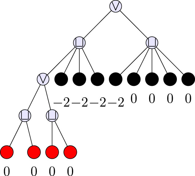
Finally, for the last iteration, we have coduplicate vertices with assignments − 2 7 and 0. Since α + β ≠ − 2 , the subcase 1a is executed and the assignments − 7 12 and 12 7 are given. Therefore, the final diagonal is D = [ 0 , 0 , 2 , − 4 , − 3 , − 7 6 , 0 , 0 , 0 , 0 , − 7 12 , 12 7 ] .

According to Theorem 2.1, there are two Laplacian eigenvalues greater than 7, four Laplacian eigenvalues less than 7 and 7 is a Laplacian eigenvalue with multiplicity 6. In fact, L - spec ( G ) = { 12 , 9 , 7 6 , 5 3 , 0 } .

$Figure 2 Initial T G {T}_{G} with d i = d ( v i ) + x {d}_{i}=d\left({v}_{i})+x .$

Figure 2

Initial T G with d i = d ( v i ) + x .

Figure 3

The first iteration.

Figure 4

After subcase 2b applied.

Figure 5

After subcase 1a applied.

Figure 6

After subcase 2a applied.

Figure 7

The last iteration.

Lemma 2.1

Let G be a cograph with cotree T G . Let t i ≥ 2 be the leaves of an interior vertex w i of T G . By initializing the diagonalization algorithm with x = − d ( v i ) (respectively, x = − d ( v i ) − 1 ) for duplicate (respectively, coduplicate) vertices v i d ( v i ) (respectively, d ( v i ) + 1 ) is a Laplacian eigenvalue with multiplicity t i − 1 , if w i = ⊔ -type (respectively, w i = ∨ -type).

Proof

Let t i ≥ 2 be the leaves with degree d ( v i ) of an interior vertex w i of T G . Initializing the diagonalization algorithm with x = − d ( v i ) (respectively, x = − d ( v i ) − 1 ) for duplicate (respectively, coduplicate) vertices v i and since β = 0 (respectively, β = − 1 ), the algorithm enters to the subcase 2b (respectively, subcase 1b). Therefore, it assigns t i − 1 permanent null values.□

Lemma 2.2

Let G be a connected cograph with cotree T G . The diagonalization ( T G , x = 0 ) assigns a permanent null value in the last iteration by subcase 1a.

Proof

Let G be a connected cograph with cotree T G . Let x = 0 be a Laplacian eigenvalue of G and consider the execution of diagonalization ( T G , x = 0 ) . According Theorem 2.1, we must have a zero on the final diagonal. So, the permanent null value is given by either situations: subcase 1b, subcase 2b, or subcase 1a in the last iteration.

We assume that subcase 1b or subcase 2b are executed in an intermediate step of diagonalization ( T G , x = 0 ) . Let us denote by T G i the subcotree which has assigned this permanent zero. Let H be a connected cograph with a cotree T H obtained from T G by attaching a copy of T G i and consider the diagonalization ( T H , x = 0 ) . Since we will have two permanent null values, this is a contradiction. Therefore, it follows that permanent null value is assigned by subcase 1a in the last iteration.□

3 A linear algorithm for obtaining L - spec ( G )

In this section, we present an O ( n ) time and space algorithm for computing the Laplacian eigenvalues of a cograph G . Our approach uses the cotree T G of cograph G to perform this procedure.

The algorithm’s input is a cotree T G with vertices (including the interior vertices) having a weight. It initializes with all leaves having a weight p i = 1 and the interior vertices w i with degree δ ( w i ) (see Definition 3.1). At each iteration, a set { v 1 , … , v m } of duplicate or coduplicate vertices with maximum depth is selected. Then they are processed, that is, assignments are given to them. The assignments given to v 1 , … , v m − 1 correspond to a Laplacian eigenvalue of G , while the vertex v m receives the value ∑ i p i . Then v 1 , … , v m − 1 are removed from the T G , which means that v 1 , … , v m − 1 have a permanent final value. The vertex v m is relocated under its parents, and then the algorithm moves to the cotree T G − { v 1 , … , v m − 1 } . This process is repeated until we obtain a cotree with only one leaf. We consider the following definition.

Definition 3.1

Let G be a cograph with cotree T G having r interior vertices { w 1 , … , w r } . We assume that leaves of an interior vertex w i have vertices v i with a weight p i . For a fixed j ∈ { 1 , … , r } , the degree of an interior vertex w j , denoted by δ ( w j ) , is given by

δ ( w j ) = ∑ i p i

sum being over i ′ s with lca ( w i , w j ) = ∨ .

Proposition 3.1

Let G be a cograph of order n with cotree T G having r interior vertices { w 1 , … , w r } . We assume that leaves t i ≥ 1 of an interior vertex w i have vertices v i with a weight p i = 1 . For any interior vertex w j , j ∈ { 1 , … , r } , we have

δ ( w j ) = t j + ∑ i t i , i f w j = ∨ , s u m b e i n g o v e r i ′ s w i t h lca ( w i , w j ) = ∨ , ∑ i t i , i f w j = ⊔ , s u m b e i n g o v e r i ′ s w i t h lca ( w i , w j ) = ∨ .

Furthermore, for j ∈ { 1 , … , r } , holds

n = δ ( w j ) + δ ( w j ¯ ) ,

where w j ¯ is the respective interior vertex of w j with opposite type in the cotree T G ¯ .

Proof

Let G be a cograph of order n with cotree T G having r interior vertices { w 1 , … , w r } . We assume that leaves t i ≥ 1 of an interior vertex w i have vertices v i with a weight p i = 1 . Let w j be an interior vertex with δ ( w j ) . By definition, we have that δ ( w j ) = ∑ i p i sum being over i ′ s with lca ( w i , w j ) = ∨ . So, if w j = ⊔ then δ ( w j ) is equivalent to sum t i , which have with w j a least common ancestor of ∨ -type since the leaves of cotree have weight p i = 1 . Otherwise, if w j = ∨ and it has t j ≥ 1 leaves with a weight p j = 1 , then ∑ j t j must be included in δ ( w j ) since the lca ( w j , w j ) = w j .

In relation to the second statement, we first note that δ ( w j ) ≤ n , for any interior vertex w j ∈ T G . Let p ≥ 0 be an integer such that n = p + δ ( w j ) . Since p represents the number of leaves t i of w i ∈ T G with lca ( w i , w j ) = ⊔ , including the t j leaves of w j , if w j = ⊔ -type, then p = δ ( w j ¯ ) , where w j ¯ is the respective interior vertex of w j with opposite type in the cotree T G ¯ and therefore, follows the result.□

Lemma 3.1

Let G be a cograph of order n with cotree T G . We assume that the leaves of T G have initialized with weight p i = 1 and the interior vertices w i with degree δ ( w i ) . If w j is an interior vertex with maximum depth in T G with t j ≥ 2 leaves having vertices with weight p j then δ ( w j ) is a Laplacian eigenvalue of G with multiplicity t j − 1 .

Proof

Let G be a cograph of order n with cotree T G . We assume that leaves of T G have initialized with weight p i = 1 and the interior vertices with degree δ ( w i ) . Let w j be an interior vertex with maximum depth in T G with t j ≥ 2 leaves having vertices with weight p j . We claim that δ ( w j ) is a Laplacian eigenvalue of G with multiplicity t j − 1 . For getting the result, it suffices to show that diagonalization ( T G , x = − δ ( w j ) ) assigns t j − 1 permanent zeros after processing t j leaves. We consider the following cases:

Case 1. If w j = ⊔ . If w j is a terminal vertex of T G , in this case, we have that δ ( w j ) coincides with the degree of vertices in the leaves t j according to Proposition 3.1, and hence, the result follows according to Lemma 2.1. If w j is not a terminal vertex of T G , we have that some leaves have been processed previously. Since duplicate vertices assign a permanent value zero if and only if the subcase 2b occurs, then duplicate vertices must receive the value zero from coduplicate vertices during their last iteration. Let us denote T H i the subcotree of T G , where w i has been an immediate successor of w j having t i leaves, such that to process their leaves, t i has a pendant vertex with assignment zero. Taking into account that leaves of T H i have initialized with d ( v i ) + δ ( w j ) − δ ( w j ) , where d ( v i ) is the degree of leaves t i only in the subcotree T H i , and this is equivalent to apply the diagonalization ( T H i , x = 0 ) . So, by Lemma 2.2, we will have t j duplicate vertices with assignment equal to zero. Therefore, t j − 1 zeros will be assigned, as desired.

Case 2. If w j = ∨ . Consider the complement graph G ¯ and its cotree T G ¯ . Let w j ¯ be the respective vertex of w j with opposite type in T G ¯ having t j leaves. By previous case, δ ( w j ¯ ) is a Laplacian eigenvalue of G ¯ with multiplicity t j − 1 . By Proposition 3.1, we have n − δ ( w j ¯ ) = δ ( w j ) , and therefore, δ ( w j ) is a Laplacian eigenvalue of G with multiplicity t j − 1 , as desired.□

Algorithm 2. Algorithm L -eigenvalues
Require: cotree T G with values p i and δ ( w i )
Ensure: L -eingenvalues of G
initialize p i = 1
while T G has ≥ 2 leaves do
select { v 1 , … , v m } (co)duplicate of maximum depth with parent w having δ ( w )
if T G has depth ≥ 2 then
v 1 , … , v m − 1 ← δ ( w )
v m ← ∑ i p i
T G = T G − { v 1 , … , v m − 1 }
else if T G has depth 1 then
v 1 , … , v m − 1 ← δ ( w )
v m ← 0
T G = T G − { v 1 , … , v m − 1 }
end if
end while

The next result claims that the algorithm L -eigenvalues computes the Laplacian eigenvalues of cograph G directly from T G in O ( n ) time and space.

Given a weighted cotree T G where the leaves have initialized with value p i = 1 and the interior vertices with their degrees δ ( w i ) . The Algorithm L -eigenvalues performs directly on the leaves of T G , which makes the procedure linear in the number of leaves. Furthermore, in each iteration, it records changes of the values on it such that the removed vertices { v 1 , … , v m − 1 } represent a Laplacian eigenvalue of G with multiplicity m − 1 , while that remaining vertex v m with value ∑ i p i , which preserves the degrees of remaining interior vertices in T G − { v 1 , … , v m } , allowing only O ( n ) space.

Theorem 3.1

Let G be a cograph of order n with cotree T G having depth l ≥ 1 . We assume that leaves t i of T G have initialized with weight p i = 1 and the interior vertices with degree δ ( w i ) . The Laplacian eigenvalues of G can be computed in O ( n ) time and space by the algorithm L-eigenvalues and they are given by

δ ( w j ) with multiplicity t j − 1 , if l ≥ 2 , w j = { ∨ , ⊔ } and t j ≥ 2 .
δ ( w j ) and 0 with multiplicities t j − 1 and 1, if l = 1 , w j = { ∨ , ⊔ } and t j ≥ 2 .

Proof

Let G be a cograph of order n with cotree T G having depth l ≥ 1 . We assume that leaves t i of T G have initialized with weight p i = 1 and the interior vertices with degree δ ( w i ) . We prove by induction on depth l ≥ 1 .

For l = 1 , we have to consider two cases. If w j = ⊔ with n = t j leaves having vertices with weight p j = 1 . Since δ ( w j ) = 0 , we have that 0 is a Laplacian eigenvalue with multiplicity n = t j . If w j = ∨ with n = t j leaves having vertices with weight p j = 1 . Since δ ( w j ) = ∑ j p j = n , then n and 0 are the Laplacian eigenvalues of G with multiplicity t j − 1 = n − 1 and 1, respectively.

Now, we suppose that algorithm L -eigenvalues holds for a cograph G with cotree T G having depth ≤ l . Let G ′ be a cograph where cotree T G ′ has depth equal to l + 1 . If l + 1 is even (respectively, odd), then T G ′ has t j leaves of an interior vertex w j = ⊔ (respectively, w j = ∨ ), which are duplicate (respectively, coduplicate) vertices. By Lemma 3.1, δ ( w j ) is a Laplacian eigenvalue with multiplicity t j − 1 . Since the pending vertex is relocated under its parents, the algorithm moves to the cotree, which has a depth equal to l . Then by applying the induction on cotree, this completes the proof of theorem.□

Example 3.1

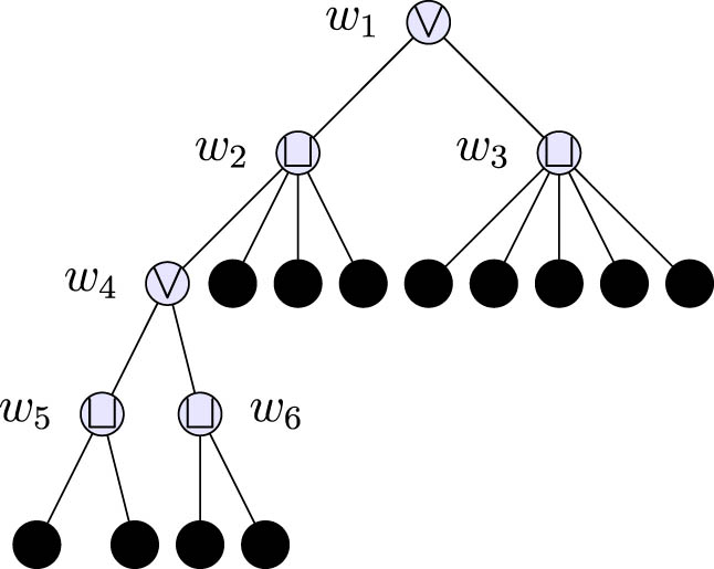
We consider the cograph G = ( ( K ¯ 2 ∨ K ¯ 2 ) ⊔ K ¯ 3 ) ∨ K ¯ 5 with cotree T G as illustrated in Figure 8. We will show that L - spec ( G ) = { 12 , 9 , 7 6 , 5 3 , 0 } .

The algorithm L -eigenvalues initializes the leaves of T G with p i = 1 and the interior vertices with δ ( w i ) . In each iteration, a set of duplicate or coduplicate vertices selected appear in blue.

In the first iteration of the algorithm, duplicate vertices { v 1 , v 2 } are chosen of w i with maximum depth, as illustrated in Figure 9. Since δ ( w i ) = 7 , the assignments are given

v 1 ← 7 ; v 2 ← 1 + 1 = 2 ; T G = T G − { v 1 } .

Then the vertex v 1 is removed and v 2 is relocated under its parents, as illustrated in Figure 10. It means that 7 is a Laplacian eigenvalue with multiplicity one.

In the next step, again duplicate vertices { v 1 , v 2 } are chosen of w i with maximum depth. Since δ ( w i ) = 7 , the assignments are given

v 1 ← 7 ; v 2 ← 1 + 1 = 2 ; T G = T G − { v 1 } .

Then the vertex v 1 is removed and v 2 is relocated under its parents, as illustrated in Figure 11. It means that 7 is a Laplacian eigenvalue with multiplicity one.

In the next step, a pair of coduplicate vertices { v 1 , v 2 } of depth three is chosen. Since δ ( w i ) = 9 and the vertices have weights p i = 2 , the following assignments are made:

v 1 ← 9 ; v 2 ← 2 + 2 = 4 ; T G = T G − { v 1 } .

Figure 12 shows the cotree with v 1 removed and v 2 relocated. It means that 9 is a Laplacian eigenvalue with multiplicity one. Next, a set of duplicate vertices { v 1 , v 2 , v 3 , v 4 } with depth two is selected, as illustrated in Figure 12. Since δ ( w i ) = 5 , we have the following assignments:

v 1 , v 2 , v 3 ← 5 ; v 4 ← 4 + 1 + 1 + 1 = 7 ; T G − { v 1 , v 2 , v 3 } .

Figure 13 shows the cotree with { v 1 , v 2 , v 3 } removed and v 4 relocated. It means that 5 is a Laplacian eigenvalue with multiplicity 3. Next, another depth two of duplicate vertices { v 1 , v 2 , v 3 , v 4 , v 5 } is selected. Since δ ( w i ) = 7 , we have the following assignments:

v 1 , v 2 , v 3 , v 4 ← 7 ; v 5 ← 1 + 1 + 1 + 1 + 1 = 5 ; T G − { v 1 , v 2 , v 3 , v 4 } .

Figure 14 shows the cotree with { v 1 , v 2 , v 3 , v 4 } removed and v 5 relocated. It means that 7 is a Laplacian eigenvalue with multiplicity 4.

Finally, the last step of Algorithm L -eigenvalues is to process the coduplicate vertices { v 1 , v 2 } with assignments p 1 = 7 and p 2 = 5 , as illustrated in Figure 14. Since the cotree has depth 1 and δ ( w i ) = 12 , we have the following assignments:

v 1 ← 12 ; v 2 ← 0 .

It means that 12 and 0 are Laplacian eigenvalues with multiplicities one. This step is illustrated in Figure 15. The algorithm stops, since the cotree has only one leaf, and we have that L - spec ( G ) = { 12 , 9 , 7 6 , 5 3 , 0 } .

$Figure 8 Initial T G {T}_{G} with p i = 1 {p}_{i}=1 and δ ( w i ) . \delta \left({w}_{i}).$

Figure 8

Initial T G with p i = 1 and δ ( w i ) .

Figure 9

The first iteration.

Figure 10

The second iteration.

Figure 11

The third iteration.

Figure 12

The fourth iteration.

Figure 13

The fifth iteration.

Figure 14

The sixth iteration.

Figure 15

The final step.

4 The number of spanning trees of a cograph

We recall that a spanning tree of a connected undirected graph G on n vertices is a connected ( n − 1 ) -edge subgraph of G .

We finalize this article using the algorithm L -eigenvalues as a tool for obtaining a closed formula for the number of spanning trees of a cograph.

The following result is due to [16].

Lemma 4.1

Let G be a connected graph on n vertices, and let L ( G ) be its Laplacian matrix. Let 0 = μ 1 ≤ μ 2 ≤ … ≤ μ n be the eigenvalues of L ( G ) . Then the number of spanning trees of G equals the product μ 2 … μ n ⁄ n .

Theorem 4.1

Let G be a connected cograph on n vertices with cotree T G having r interior vertices { w 1 , … , w r } . Let w 1 be the cotree’s root and suppose that any interior vertex w i of T G has s i successors vertices and t i leaves. Then the number of spanning trees of G equals

n s 1 + t 1 − 2 ∏ i = 2 r ( δ ( w i ) ) s i + t i − 1 .

Proof

Let G be a connected cograph on n vertices with cotree T G having r interior vertices { w 1 , … , w r } . We assume that w 1 is the cotree’s root and each w i has s i successors vertices and t i leaves. It is sufficient to show that δ ( w i ) corresponds to a Laplacian eigenvalue of G with multiplicity s i + t i − 1 .

If w i = ⊔ and it is a terminal vertex, we have that δ ( w i ) coincides with the degree of vertices in the leaves t i . So, by Lemma 2.1, we are done. Now, if w i is not a terminal vertex, we have that w i has s i successors vertices and t i leaves. After the algorithm L -eigenvalues processes the s i interior vertices, by Lemma 3.1, δ ( w i ) corresponds to a Laplacian eigenvalue of G with multiplicity s i + t i − 1 . The proof is analogous for an interior vertex w i of ∨ -type.

To finish, we need to account the Laplacian eigenvalue given by the interior vertex of cotree’s root. Let w 1 = ∨ be the interior vertex of cotree’s root of T G having s 1 successors vertices and t 1 leaves. Since the algorithm L -eigenvalues assigns to w 1 the Laplacian eigenvalue n with multiplicity s 1 + t 1 − 1 , and according Lemma 4.1, we must divide the product of Laplacian eigenvalues by factor n , where n is a factor with multiplicity s 1 + t 1 − 2 , as desired.□

As illustration, we exhibit an example for obtaining the number of spanning trees of a cograph.

Example 4.1

Let G be a cograph having cotree T G , as illustrated in the Figure 16.

We have that T G has a set of interior vertices { w 1 , w 2 , w 3 , w 4 , w 5 , w 6 } , where w 1 is the cotree’s root of T G . Computing the degrees of interior vertices and their respective number of successors vertices and leaves, we have

δ ( w 1 ) = 12 , s 1 = 2 , t 1 = 0 ; δ ( w 2 ) = 5 , s 2 = 1 , t 2 = 3 ; δ ( w 3 ) = 7 , s 3 = 0 , t 3 = 5 ; δ ( w 4 ) = 9 , s 4 = 2 , t 4 = 0 ; δ ( w 5 ) = 7 , s 5 = 0 , t 5 = 2 ; δ ( w 6 ) = 7 , s 6 = 0 , t 6 = 2 ;

By Theorem 4.1, we have the number of spanning trees of G equals

( 5 ) 3 ⋅ ( 7 ) 4 ⋅ ( 9 ) 1 ⋅ ( 7 ) 1 ⋅ ( 7 ) 1 ⋅ ( 12 ) 0 .

$Figure 16 The cotree T G . {T}_{G}.$

Figure 16

The cotree T G .

Acknowledgements

This work was part of the Post-Doctoral studies of Fernando C. Tura, while visiting Georgia State University, on leave from UFSM and supported by CNPq Grant 200716/2022-0. Guantao Chen acknowledges partial support of NSF grant DMS-2154331.

Author contributions: Guantao Chen: Conceptualization, Formal analysis, Supervision, Investigation, Methodology, Validation, Writing – original draft, Writing – review & editing. Fernando C. Tura: Conceptualization, Formal analysis, Funding acquisition, Investigation, Methodology, Project administration, Validation, Writing – original draft, Writing – review & editing.
Conflict of interest: The authors state no conflict of interest.
Data availability statement: Not applicable.

References

[1] N. Abreu, C. M. Justel, and L. Markenzon, Integer Laplacian eigenvalues of chordal graphs, Linear Algebra Appl. 614 (2021), 68–81. 10.1016/j.laa.2019.12.030Search in Google Scholar

[2] L. E. Allem and F. C. Tura, Multiplicity of eigenvalues of cographs, Discrete Appl. Math. 247 (2018), 43–52. 10.1016/j.dam.2018.02.010Search in Google Scholar

[3] L. E. Allem and F. C. Tura, Integral cographs, Discrete Appl. Math. 283 (2020), 153–167. 10.1016/j.dam.2019.12.021Search in Google Scholar

[4] M. Andelić, Z. Du, C. M. da Fonseca, and S. K. Simić, Tridiagonal matrices and spectral properties of some graph classes, Czech. Math. J. 70 (2020), 1125–1138. 10.21136/CMJ.2020.0182-19Search in Google Scholar

[5] R. B. Bapat, A. K. Lal, and S. Pati, Laplacian spectrum of weakly quasi-threshold graphs, Graphs Combin. 24 (2008), 273–290. 10.1007/s00373-008-0785-9Search in Google Scholar

[6] T. Bíyíkoğlu, S. K. Simić, and Z. Stanić, Some notes on spectra of cographs, Ars Combin. 100 (2011), 421–434. Search in Google Scholar

[7] A. Brandstadt, V. B. Le, and J. P. Spinrad, Graph classes: A survey. In: SIAM Monographs on Discrete Mathematics and Applications, 1999. 10.1137/1.9780898719796Search in Google Scholar

[8] A. Bretscher, D. Corneil, M. Habib, and C. Paul, A simple linear time LexBFS cograph recognition algorithm. SIAM J. Discrete Math. 22 (2008), 1277–1296. 10.1137/060664690Search in Google Scholar

[9] D. G. Corneil, H. Lerchs, and L. B. Stewart, Complement reducible graphs, Discrete Appl. Math. 3 (1981), 163–174. 10.1016/0166-218X(81)90013-5Search in Google Scholar

[10] D. G. Corneil, Y. Perl, and L. B. Stewart, A linear recognition algorithm for cographs, SIAM J. Comput. 14 (1985), no. 4, 926–934. 10.1137/0214065Search in Google Scholar

[11] M. C. Golumbic, Algorithmic graph theory and perfect graphs, 2nd edn. In: Annals of Discrete Mathematics, vol. 57. Elsevier, Amsterdam, 2004. 10.1016/S0167-5060(04)80051-7Search in Google Scholar

[12] M. Habib and C. Paul, A simple linear time algorithm for cograph recognition, Discrete Appl. Math. 145 (2005), no. 2, 183–197. 10.1016/j.dam.2004.01.011Search in Google Scholar

[13] D. P. Jacobs, V. Trevisan, and F. C. Tura, Eigenvalue location in cographs, Discrete Appl. Math. 245 (2018), 220–235. 10.1016/j.dam.2017.02.007Search in Google Scholar

[14] Y. Jing-Ho, C. Jer-Jeong, and J. C. Gerard, Quasi-threshold graphs, Discrete Appl. Math. 69 (1996), 247–255. 10.1016/0166-218X(96)00094-7Search in Google Scholar

[15] A. Jones, V. Trevisan, and C. T. M. Vinagre, Exploring symmetries in cographs: Obtaining spectra and energies, Discrete Appl. Math. 325 (2023), 120–133. 10.1016/j.dam.2022.10.002Search in Google Scholar

[16] A. K. Kelmans and V. M. Chelnokov, A certain polynomial of a graph and graphs with an extremal number of trees. J. Combin. Theory B 16 (1974), 197–214. 10.1016/0095-8956(74)90065-3Search in Google Scholar

[17] J. Lazzarin, O. F. Márquez, and F. C. Tura, No threshold graphs are cospectral, Linear Algebra Appl. 560 (2019), 133–145. 10.1016/j.laa.2018.09.033Search in Google Scholar

[18] J. Lazzarin, O. F. Sosa, and F. C. Tura, Laplacian eigenvalues of equivalent cographs, Linear Multilinear Algebra 71 (2022), no. 6, 1003–1014. 10.1080/03081087.2022.2050168Search in Google Scholar

[19] N. V. R. Mahadev and U. N. Peled, Threshold graphs and related topics, 1st edn. In: Annals of discrete mathematics, vol. 56, North-Holland, New York, 1995. Search in Google Scholar

[20] S. Mandal, R. Mehatari, and Z. Stanić, Laplacian eigenvalues and eigenspaces of cographs generated by finite sequence. Indian J. Pure Appl. Math. (2024).10.1007/s13226-024-00572-wSearch in Google Scholar

[21] R. Merris, Degree maximal graphs are Laplacian integral, Linear Algebra Appl. 199 (1994), 381–389. 10.1016/0024-3795(94)90361-1Search in Google Scholar

[22] S. S. Mousavi, M. Haeri, and M. Mesbahi, Laplacian dynamics on cographs: Controllability analysis through joins and unions, IEEE Trans Automatic Control 66 (2021), no. 3, 1383–1390. 10.1109/TAC.2020.2992444Search in Google Scholar

[23] S. D. Nikolopoulos and C. Papadopoulos, Counting spanning trees in cographs: an algorithmic approach, Ars Combin. 90 (2009). 257–274Search in Google Scholar

[24] S. D. Nikolopoulos and C. Papadopoulos, A simple linear-time recognition algorithm for weakly quasi-threshold graphs, Graphs Combin. 27 (2011), 557–565. 10.1007/s00373-010-0983-0Search in Google Scholar

Received: 2024-03-27

Revised: 2024-08-06

Accepted: 2024-08-07

Published Online: 2024-09-06

This work is licensed under the Creative Commons Attribution 4.0 International License.

Articles in the same Issue

https://doi.org/10.1515/spma-2024-0024

Keywords for this article

cograph; Laplacian eigenvalues; spanning trees

Creative Commons

BY 4.0