Computing the matrix exponential with the double exponential formula
-
Fuminori Tatsuoka
 ,
Tomohiro Sogabe
,
Tomohiro Sogabe

Abstract
This article considers the computation of the matrix exponential
1 Introduction
The exponential of a matrix
and it arises in several situations in scientific computing. One of the applications is the exponential integrator, a class of numerical solvers for stiff ordinary differential equations [13]. In recent years,
In general, quadrature-based methods have two advantages: these algorithms can compute
Quadrature-based algorithms in [5,24] focus on (nearly) Hermitian matrices. In detail, they are proposed for the efficient computation of Bromwich integrals whose integrand has singularities on or near the negative real axis. For the computation of
The motivation of this study is to construct quadrature-based algorithms that can be used for non-Hermitian matrices. Here, we consider another integral representation
The derivation of (1) is presented in A. The integral representation (1) holds when all the eigenvalues of
Since the integrand in (1) includes an oscillatory term
In this article, we propose algorithms using the DE formula to compute
The organization of this article is as follows: The DE formula used in this article is introduced in Section 2. In Section 3, we analyze the truncation error and propose algorithms. Numerical results are presented in Section 4, and we conclude this article in Section 5.
2 The DE formula for Fourier integrals
The DE formula exploits the fact that the trapezoidal rule for the integrals of analytic functions on the real line converges exponentially [20]. Several types of change of variable are proposed to deal with different types of integrals. In [16], integral forms of
are considered, where
The DE formula for (2) is as follows. We first select the mesh size
The summand decays double exponentially as
which is proposed in [16], or
which is proposed in [17]. The implementation notes for (3) is presented in Appendix B.
The DE formula can be applied to (1) because the integrand is a rational function of
3 Computing
e
A
with the DE formula
In this section, we propose algorithms for
where
We may not write the second argument of
The error of the DE formula can be divided into the discretization error and the truncation error:
We employ a posteriori error estimation technique to presume the discretization error and provide an upper bound on the truncation error. In Section 3.1, we analyze the truncation error for the given interval, and in Section 3.2, we present the two algorithms; notably, one algorithm uses the technique to achieve the required accuracy.
3.1 Truncation error
We show an upper bound on the truncation error as follows:
Proposition 1
Suppose that all the eigenvalues of
where
Proof
From the triangle inequality, it holds that
In this proof, we show (5) that
We first show (6). The assumption
In addition, because
Next, we show (7). It is easily seen that
Here, because
We remark that the transformation (3) satisfies
3.2 Algorithms
In this subsection, we propose two algorithms. The first one computes
In the first algorithm, the input matrix
|
Algorithm 1 Computing
|
|
|---|---|
|
Input
|
|
| 1: | Compute the right-most eigenvalue of
|
| 2: |
|
| 3: |
|
| 4: |
|
|
Output
|
|
| 5: |
function GetInterval
|
| 6: |
|
| 7: |
|
| 8: |
|
| 9: | end function |
Algorithm 1 requires the shift parameter
The computation of the resolvent
for accuracy.
To obtain an upper bound on the 2-norm of the truncation error using Proposition 1, it is necessary to compute the norm
Hence, for highly non-normal matrices such that
The infinite sums in steps 6 and 7 of Algorithm 1 can be approximated without too much computations because the summands
We next propose an automatic quadrature algorithm. Ooura and Mori proposed an automatic quadrature algorithm in [17, Section 5] that is applicable when the convergence rate of the DE formula, the constant
In the computation of
In the algorithm, we first select three mesh sizes
By solving
and we can approximate
|
Algorithm 2 Automatic quadrature algorithm for
|
|
|---|---|
|
Input
|
|
|
Output
|
|
| 1 : | Compute the rightmost eigenvalue of
|
| 2 : |
|
| 3 : |
|
| 4: |
|
| 5: |
|
| 6: |
|
| 7: |
|
| 8: |
|
| 9: |
if
|
| 10: |
|
| 11: | else |
| 12: |
|
| 13: |
|
| 14: |
|
| 15: |
|
| 16: |
|
| 17: |
|
| 18: |
|
| 19: |
|
| 20: |
|
| 21: |
|
| 22: |
|
| 23: | end if |
4 Numerical examples
The computation is carried out with Julia 1.10.0 on an Intel Core i5-9600K CPU with 32 GB RAM. The IEEE double-precision arithmetic is used unless otherwise stated. The reference solutions in Section 4.5 are computed by
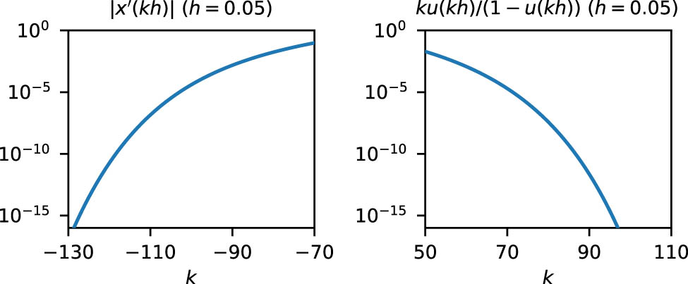
4.1 Computing the scalar exponential with the DE formula
By using the result in [3], the upper bound on the error of the DE formula can be obtained by
When
When
When
The error of the double exponential formula for the scalar exponential
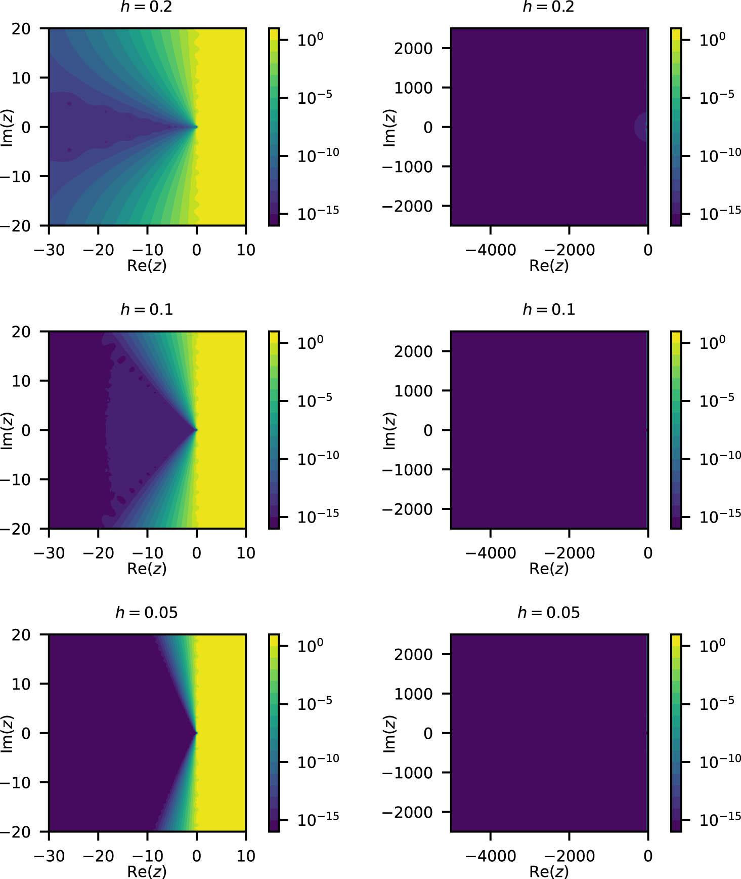
4.2 Accuracy dependence on the shift parameter
σ
Algorithm 1 requires the parameter
Figure 3 shows the error of the DE formula for

Accuracy dependence of the double exponential formula on the shift parameter
4.3 Accuracy control of automatic quadrature
Here, we see the accuracy control of Algorithm 2. Figure 4 shows the error of Algorithm 2, where the test matrices are the same as in Section 4.2, and the safe parameter is set to
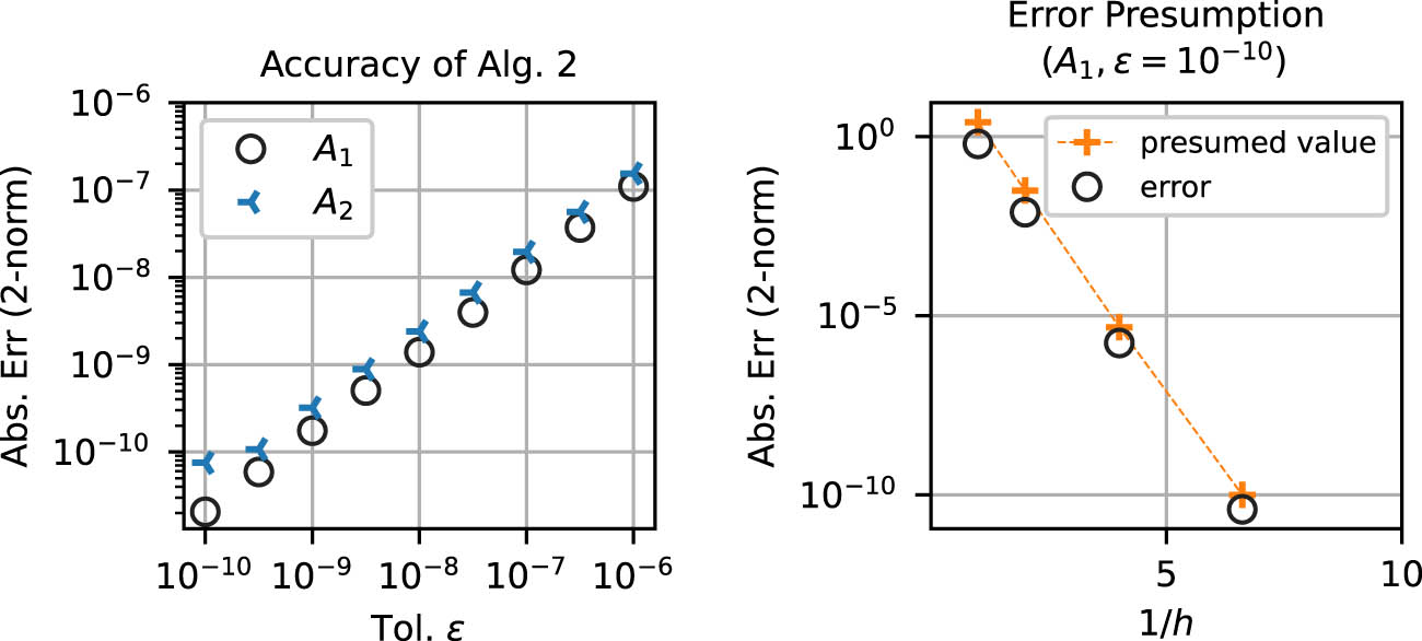
The accuracy of Algorithm 2. The left figure shows the accuracy dependence on the input tolerance
The left figure shows the accuracy dependence on the input tolerance
4.4 Accuracy of Algorithm 2
In this example, we compute the exponential of 51 test matrices from MatrixDepot.jl [25]. The size of these matrices is
Figure 5 shows the error of this example. It is observed that the error of Algorithm 2 is less than
![Figure 5
The error
‖
X
‒
e
A
′
‖
2
\Vert X‒{{\rm{e}}}^{A^{\prime} }{\Vert }_{2}
of Algorithm 2 and exp function in Julia, which uses the scaling and squaring algorithm in [11].](/document/doi/10.1515/spma-2024-0013/asset/graphic/j_spma-2024-0013_fig_005.jpg)
The error
4.5 A comparison of the DE formula with the Cauchy integral for non-Hermitian matrices
In this example, we compute
The matrices are generated from the convection-diffusion problems
where
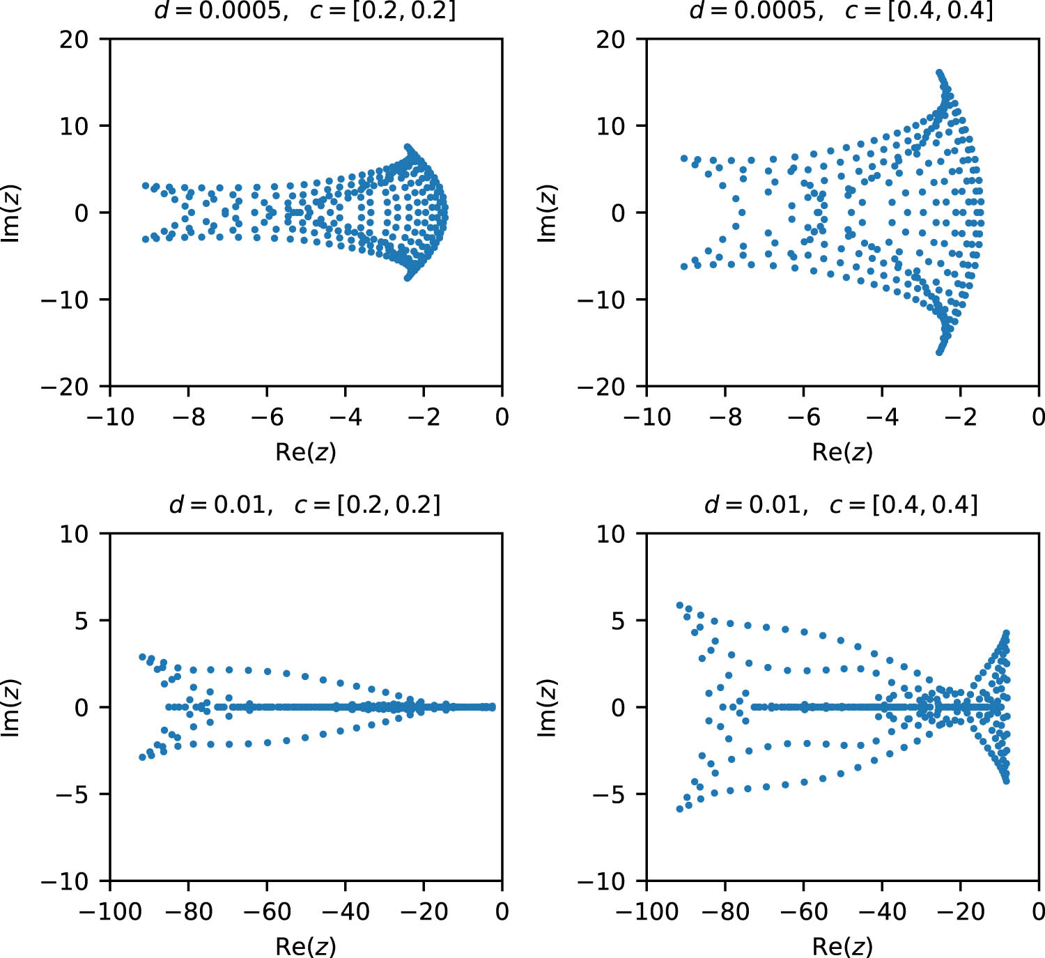
Eigenvalues of the test matrix
For DE, we set
where
where
Figure 7 illustrates the convergence histories of these algorithms for
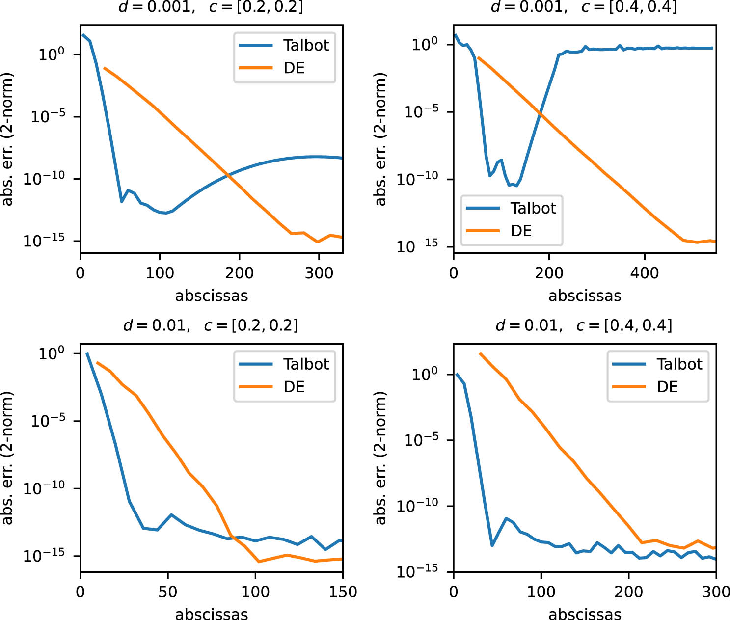
Convergence histories of DE and Talbot for the problem
5 Conclusion
The DE formula was considered for the computation of
Future work includes improvement of the change of variable of the DE formula for
Acknowledgements
The authors are grateful to the two anonymous referees for the careful reading and the comments that substantially enhanced the quality of the manuscript.
-
Funding information: This work was supported by JSPS KAKENHI Grant Numbers 20H00581 and 20K20397. The authors would like to thank Enago (www.enago.jp) for English language editing.
-
Author contributions: Fuminori Tatsuoka: conceptualization, experimentation, writing – original draft; Tomohiro Sogabe: writing – review and editing, supervision; Tomoya Kemmochi: writing – review and editing, supervision; Shao-Liang Zhang: writing – review and editing, supervision.
-
Conflict of interest: The authors declare no conflicts of interest.
-
Data availability statement: All data that support this study are available at GitHub https://github.com/f-ttok/article-expmde.
Appendix A Derivation of the integral representation (1)
From [6, p. 758], it holds that
where
where all the eigenvalues of
where
B Derivative of the change of variable
Let
Because
When
Experimentally, the value
The value of
|
|
|
|---|---|
|
|
0.493 |
|
|
0.514 |
|
|
0.524 |
|
|
0.526 |
References
[1] A. H. Al-Mohy and N. J. Higham, A new scaling and squaring algorithm for the matrix exponential, SIAM J. Matrix Anal. Appl. 31 (2009), no. 3, 970–989. 10.1137/09074721XSearch in Google Scholar
[2] A. H. Al-Mohy and N. J. Higham, Computing the action of the matrix exponential, with an application to exponential integrators, SIAM J. Sci. Comput. 33 (2011), no. 2, 488–511. 10.1137/100788860Search in Google Scholar
[3] M. Crouzeix and C. Palencia, The numerical range is a (1+2)-spectral set, SIAM J. Matrix Anal. Appl. 38 (2017), no. 2, 649–655. 10.1137/17M1116672Search in Google Scholar
[4] O. De la Cruz Cabrera, M. Matar, and L. Reichel, Analysis of directed networks via the matrix exponential, J. Comput. Appl. Math. 355 (2019), 182–192. 10.1016/j.cam.2019.01.015Search in Google Scholar
[5] B. Dingfelder and J. A. C. Weideman, An improved Talbot method for numerical Laplace transform inversion, Numer Algor, 68 (2015), no. 1, 167–183. 10.1007/s11075-014-9895-zSearch in Google Scholar
[6] V. Druskin and L. Knizhnerman, Extended Krylov subspaces: Approximation of the matrix square root and related functions, SIAM J. Matrix Anal. Appl. 19 (1998), no. 3, 755–771. 10.1137/S0895479895292400Search in Google Scholar
[7] M. Fasi and N. J. Higham, An arbitrary precision scaling and squaring algorithm for the matrix exponential, SIAM J. Matrix Anal. Appl. 40 (2019), no. 4, 1233–1256. 10.1137/18M1228876Search in Google Scholar
[8] T. Göckler and V. Grimm, Uniform approximation of ϕ-functions in exponential integrators by a rational krylov subspace method with simple poles, SIAM J. Matrix Anal. Appl. 35 (2014), no. 4, 1467–1489. 10.1137/140964655Search in Google Scholar
[9] S. Güttel and Y. Nakatsukasa, Scaled and squared subdiagonal Padé approximation for the matrix exponential, SIAM J. Matrix Anal. Appl. 37 (2016), no. 1, 145–170. 10.1137/15M1027553Search in Google Scholar
[10] F. Hecht, New development in FreeFem++, J. Numer. Math. 20 (2012), no. 3–4, 251–265. 10.1515/jnum-2012-0013Search in Google Scholar
[11] N. J. Higham, The scaling and squaring method for the matrix exponential revisited, SIAM J. Matrix Anal. Appl. 26 (2005), no. 4, 1179–1193. 10.1137/04061101XSearch in Google Scholar
[12] N. J. Higham, Functions of Matrices: Theory and Computation, SIAM, Philadelphia, PA, 2008. 10.1137/1.9780898717778Search in Google Scholar
[13] M. Hochbruck and A. Ostermann, Exponential integrators, Acta Numer. 19 (2010), 209–286. 10.1017/S0962492910000048Search in Google Scholar
[14] C. Moler and C. Van Loan, Nineteen dubious ways to compute the exponential of a matrix, SIAM Review 20 (1978), no. 4, 801–836. 10.1137/1020098Search in Google Scholar
[15] C. Moler and C. Van Loan, Nineteen dubious ways to compute the exponential of a matrix, twenty-five years later, SIAM Review 45 (2003), no. 1, 3–49. 10.1137/S00361445024180Search in Google Scholar
[16] T. Ooura and M. Mori, The double exponential formula for oscillatory functions over the half infinite interval, J. Comput. Appl. Math. 38 (1991), no. 1, 353–360. 10.1016/0377-0427(91)90181-ISearch in Google Scholar
[17] T. Ooura and M. Mori, A robust double exponential formula for Fourier-type integrals, J. Comput. Appl. Math. 112 (1999), no. 1–2, 229–241. 10.1016/S0377-0427(99)00223-XSearch in Google Scholar
[18] Y. Saad, Analysis of some Krylov subspace approximations to the matrix exponential operator, SIAM J. Numer. Anal. 29 (1992), no. 1, 209–228. 10.1137/0729014Search in Google Scholar
[19] T. Schmelzer and L. N. Trefethen, Evaluating matrix functions for exponential integrators via Carathéodory-Fejér approximation and contour integrals, Electron. Trans. Numer. Anal. 29 (2007), 1–18. Search in Google Scholar
[20] H. Takahasi and M. Mori, Double exponential formulas for numerical integration, Publ. Res. Inst. Math. Sci. 9 (1974), 721–741. 10.2977/prims/1195192451Search in Google Scholar
[21] F. Tatsuoka, T. Sogabe, Y. Miyatake, T. Kemmochi, and S.-L. Zhang, Computing the matrix fractional power with the double exponential formula, Electron. Trans. Numer. Anal. 54 (2021), 558–580. 10.1553/etna_vol54s558Search in Google Scholar
[22] F. Tatsuoka, T. Sogabe, Y. Miyatake, and S.-L. Zhang, Algorithms for the computation of the matrix logarithm based on the double exponential formula, J. Comput. Appl. Math. 373 (2020), 112396. 10.1016/j.cam.2019.112396Search in Google Scholar
[23] L. N. Trefethen and J. A. C. Weideman, The exponentially convergent trapezoidal rule, SIAM Rev. 56 (2014), no. 3, 385–458. 10.1137/130932132Search in Google Scholar
[24] J. A. C. Weideman and L. N. Trefethen, Parabolic and hyperbolic contours for computing the Bromwich integral, Math. Comp. 76 (2007), no. 259, 1341–1356. 10.1090/S0025-5718-07-01945-XSearch in Google Scholar
[25] W. Zhang and N. J. Higham, Matrix depot: An extensible test matrix collection for Julia, PeerJ Comput. Sci. 2 (2016), e58. 10.7717/peerj-cs.58Search in Google Scholar
© 2024 the author(s), published by De Gruyter
This work is licensed under the Creative Commons Attribution 4.0 International License.
Articles in the same Issue
- Research Articles
- The diameter of the Birkhoff polytope
- Determinants of tridiagonal matrices over some commutative finite chain rings
- The smallest singular value anomaly: The reasons behind sharp anomaly
- Idempotents which are products of two nilpotents
- Two-unitary complex Hadamard matrices of order 36
- Lih Wang's and Dittert's conjectures on permanents
- On a unified approach to homogeneous second-order linear difference equations with constant coefficients and some applications
- Matrix equation representation of the convolution equation and its unique solvability
- Disjoint sections of positive semidefinite matrices and their applications in linear statistical models
- On the spectrum of tridiagonal matrices with two-periodic main diagonal
- γ-Inverse graph of some mixed graphs
- On the Harary Estrada index of graphs
- Complex Palais matrix and a new unitary transform with bounded component norms
- Computing the matrix exponential with the double exponential formula
- Special Issue in honour of Frank Hall
- Editorial Note for the Special Issue in honor of Frank J. Hall
- Refined inertias of positive and hollow positive patterns
- The perturbation of Drazin inverse and dual Drazin inverse
- The minimum exponential atom-bond connectivity energy of trees
- Singular matrices possessing the triangle property
- On the spectral norm of a doubly stochastic matrix and level-k circulant matrix
- New constructions of nonregular cospectral graphs
- Variations in the sub-defect of doubly substochastic matrices
- Eigenpairs of adjacency matrices of balanced signed graphs
- Special Issue - Workshop on Spectral Graph Theory 2023 - In honor of Prof. Nair Abreu
- Editorial to Special issue “Workshop on Spectral Graph Theory 2023 – In honor of Prof. Nair Abreu”
- Eigenvalues of complex unit gain graphs and gain regularity
- Note on the product of the largest and the smallest eigenvalue of a graph
- Four-point condition matrices of edge-weighted trees
- On the Laplacian index of tadpole graphs
- Signed graphs with strong (anti-)reciprocal eigenvalue property
- Some results involving the Aα-eigenvalues for graphs and line graphs
- A generalization of the Graham-Pollak tree theorem to even-order Steiner distance
- Nonvanishing minors of eigenvector matrices and consequences
- A linear algorithm for obtaining the Laplacian eigenvalues of a cograph
- Selected open problems in continuous-time quantum walks
- On the minimum spectral radius of connected graphs of given order and size
- Graphs whose Laplacian eigenvalues are almost all 1 or 2
- A Laplacian eigenbasis for threshold graphs