Evaluating the efficacy of fuzzy Bayesian networks for financial risk assessment

Tingyan Xiong; Zeping Liu; Minghong Zhang

doi:10.1515/dema-2024-0032

Artikel Open Access

Evaluating the efficacy of fuzzy Bayesian networks for financial risk assessment

Tingyan Xiong , Zeping Liu und Minghong Zhang

Veröffentlicht/Copyright: 13. März 2025

Veröffentlicht von

Veröffentlichen auch Sie bei De Gruyter Brill

Informationen für Autor*innen Erkunden Sie dieses Fachgebiet

Aus der Zeitschrift Demonstratio Mathematica Band 58 Heft 1

Abstract

The demand for advanced predictive tools has surged in the intricate landscape of global financial markets. Traditional predictive tools based on crisp models offer foundational insights, while the evolving complexities in global financial markets necessitate more nuanced analytical techniques. This research delves deep into Bayesian networks (FBN) as a potential tool for financial risk prediction (FRP). Integrating the probabilistic reasoning of Bayesian Networks with the uncertainty-handling capabilities of fuzzy logic, FBNs present a promising avenue for capturing the multifaceted dynamics of financial data. A comprehensive methodology was employed, encompassing data collection, data preprocessing, and transformation. The FBN model’s construction was rooted in established methodologies, emphasizing feature selection, parameter estimation, and a systematic validation process. The model’s empirical robustness was ensured through rigorous validation and testing mechanisms. The results found that the FBN accuracy achieved a mean absolute error (MAE) of 9.78 and a root mean square error (RMSE) of 11.64, when compared to traditional models such as linear regression, which had MAE and RMSE values of 15.70 and 18.39, respectively. The obtained results illuminate the FBN’s standout performance in FRP. The FBN excels in capturing the underlying intricacies of financial data, offering unparalleled predictive accuracy. Its predictions are closer to actual average value but exhibit fewer large deviations, making it an invaluable tool in the financial analytics arsenal demonstrably outpacing traditional crisp models.

Keywords: fuzzy Bayesian networks; financial risk prediction; probabilistic reasoning; financial analytics; data-driven decision making

MSC 2010: 91-08

1 Introduction

With the increasing intricacy of global financial markets, the demand for robust and sophisticated predictive tools has never been greater. Financial institutions, policymakers, and investors are perpetually questing to navigate the complexities of the market landscape, seeking mechanisms that can anticipate risks and offer strategic insights. This dynamic, coupled with the surge in computational capabilities and data availability, underscores the pressing need for advanced analytical techniques in the realm of finance [1].

Traditional financial risk prediction (FRP) models have served as foundational pillars in financial analytics. However, as the nature of financial data evolves, with interdependencies, uncertainties, and fuzzy characteristics becoming more pronounced, these conventional tools often fall short [2]. While they offer valuable insights, their assumptions of linearity and independence can sometimes oversimplify the intricate dynamics of financial markets [3].

This study aims to analyze their application within this domain, leveraging a comprehensive methodology to assess their efficacy. Through detailed construction, validation, and testing of an fuzzy Bayesian network (FBN) model tailored to financial risk assessment, this work contributes to a nuanced evaluation of FBNs. It situates the findings within a broader landscape of predictive analytics, encompassing both the rich history of Bayesian methods and the dynamic field of machine learning (ML). This study embarks on an exploration of FBN as a potential panacea. FBNs, by design, amalgamate the probabilistic reasoning (PR) of BN with the uncertainty-handling prowess of fuzzy logic (FL). This synergy allows FBNs to encapsulate the nuances of financial data, considering both the inherent uncertainties and the intricate relationships between different financial metrics. The proposed approach involved rigorous data collection from relevant financial sources, followed by comprehensive preprocessing and transformation. The construction of the FBN model was grounded in robust methodologies, from feature selection to parameter estimation. Furthermore, the proposed study employed a rigorous validation and testing mechanism, ensuring the empirical robustness of our FBN model.

In light of the advancements in artificial intelligence (AI) and ML, our study also ventures beyond traditional comparisons to include an evaluation of contemporary ML models. Recognizing the potency of algorithms such as support vector machines, neural networks, and random forests (RF) in deciphering complex patterns in data, we juxtapose FBN’s performance with these techniques. This comparative analysis, rooted in empirical data and rigorous testing, illuminates the relative strengths and potential limitations of FBNs in the vast arena of FRP. Our findings not only underscore the nuanced capabilities of FBNs but also pave the way for a more integrated approach to financial analytics, where traditional probabilistic models and cutting-edge ML techniques coalesce to offer deeper insights into risk management.

2 Literature review

In the realm of FRP, the journey has been one of constant evolution and adaptation. From the inception of finance as an academic discipline and a practical business concern, risk prediction has been pivotal [4,5]. Risk, as a concept, has always been intertwined with the return potential, and the ability to predict and quantify it has been the holy grail of both scholars and practitioners [6].

The annals of financial history are filled with attempts to understand and predict risk. Early models of risk prediction were primarily deterministic, relying on fixed inputs to predict outputs. For example, the capital asset pricing model, developed in the 1960s, tried to establish a linear relationship between the expected return of an asset and its beta [1,2], a measure of its systematic risk. However, these models had their limitations. They assumed market efficiency, and rational investors, and often ignored transaction costs or taxes. Their determinism was both their strength and their Achilles’ heel; while they provided clarity, they often failed to capture the nuances and complexities of real-world financial markets.

In the context of FRP, traditional deterministic models have a long history of using crisp numbers, which are fixed and absolute representations of data. Despite their simplicity and clarity, these models frequently fall short of capturing the intricacies of actual and real-world financial markets [1,5]. Factors including market volatility, investor emotion, and economic shifts all have an impact on financial markets. These factors are essentially oversimplified by crisp numbers, which can result in inaccurate modeling and predictions. This drawback emphasizes how inadequate conventional deterministic methods are to deal with the complex and unpredictable nature of financial markets [2].

However, with the advent of computational power and the digital revolution, the landscape of FRP underwent a seismic shift. No longer bound by the limitations of deterministic models, scholars began to explore stochastic processes, non-linear relationships, and the role of information asymmetry in financial markets [6]. ML and AI ushered in a new era, where computational models, fed with vast amounts of data, could predict risk with unprecedented accuracy.

Bayesian networks (BNs) are probabilistic graphical models that represent a set of variables and their conditional dependencies via a directed acyclic graph. They are rooted in Bayes’ theorem, a fundamental concept in probability theory and statistics that describes the probability of an event based on prior knowledge of conditions related to the event [3]. In a BN, nodes represent the random variables and edges represent the conditional dependencies. The beauty of BN lies in its ability to provide a visual and mathematical representation of complex interdependencies [4].

Their application has been vast and varied. In finance, BN has been used to model the intricate web of factors affecting asset prices, credit risk, and market crashes. They offer a flexible framework to incorporate both quantitative data (such as stock prices or interest rates) and qualitative insights (such as investor sentiment or geopolitical events) [5,6]. This makes them particularly powerful in capturing the multifaceted nature of financial risk.

This problem is compellingly solved by FL, which allows models to include varying degrees of imprecision and uncertainty in their frameworks. Fuzzy numbers provide a more flexible representation of financial data by allowing the assertion of partial truths, in contrast to crisp numbers, which consider facts as either true or untrue. This capacity is particularly beneficial in situations when there are not clear distinctions between variables, like the range of market sentiment [5]. Fuzzy numbers allow financial models to more accurately represent reality by capturing the complex interactions of market forces. FL’s fundamental strength makes it obvious for integration with BNs, which leads to the development of FBNs as an effective tool for evaluating financial risk [6].

FL, unlike classical or Boolean logic, deals with reasoning that is approximate rather than fixed and exact. Proposed by Lotfi Zadeh in the 1960s, FL provides a mathematical tool to handle uncertainty and imprecision. In a fuzzy system, truth values are represented by degrees of membership to a fuzzy set, rather than a binary true or false [7,8,9,10].

In the financial world, where uncertainty is the only certainty, fuzzy systems have found a natural home. They have been used to model the uncertainty in financial markets, to predict stock prices, and even to design trading systems. The key advantage of fuzzy systems in finance is their ability to model imprecise information, such as investor sentiment or the likelihood of a political event, and integrate it with quantitative data [11,12,13,14].

The synthesis of FL and BN represents a convergence of two powerful paradigms. By integrating fuzzy systems with BN, one can model uncertainty and probabilistic interdependencies in a unified framework. This integration allows for the representation of imprecise knowledge and its conditional dependencies in a cohesive manner.

Numerous studies have delved into this integration, especially in the context of finance. Researchers have found that the combined model can predict financial risk with greater accuracy than either model on its own. The advantages are manifold: the ability to incorporate both quantitative and qualitative data, flexibility in modeling complex relationships, and a robust mathematical framework to underpin predictions [15].

Recent advancements in predictive analytics have emphasized the need for models that can accurately navigate the uncertainties inherent in financial data. FBNs, with their robust PR and capacity to handle ambiguity, have emerged as a significant tool across various domains beyond finance, including healthcare and engineering. Pioneering efforts have showcased FBNs’ versatility, while sector-specific applications underscore their value in financial risk assessment [3,7,16–21]. These contributions highlight FBNs’ broad adoption, challenging the notion of their novelty in financial applications. This study seeks to extend the current understanding of FBNs by providing a comprehensive analysis of their utility in FRP, set against the backdrop of both traditional models and contemporary ML techniques. Our literature review thus bridges the gap between foundational research and the cutting edge, illustrating the evolution of predictive models from deterministic frameworks to sophisticated, data-driven approaches that embrace complexity and uncertainty.

3 Research method

3.1 Data collection

In the context of FRP using FBNs, data play a paramount role. Financial data are both vast in quantity and intricate in detail. Data can emanate from multiple sources, each offering a unique lens to view the financial landscape. Among these sources are stock exchanges, which provide granular data on stock prices, trading volumes, and other market-related metrics. Financial institutions, regulatory filings, and economic databases offer insights into financial statements, credit histories, and macroeconomic indicators. In addition, sentiment analysis tools can scrape news articles, financial reports, and social media feeds to gauge market sentiment, an increasingly influential factor in financial markets.

Selecting the right data is as critical as accessing it. Given the complexity of financial markets, it is essential to have criteria that ensure the relevance and quality of data. Two primary considerations dominate this selection process:

Temporal Relevance: The period of data collection must align with the study’s objectives. For instance, if the study aims to predict short-term market risks, then high-frequency intraday data might be more relevant. Conversely, for long-term risk assessments, quarterly or yearly data might suffice.
Feature Relevance: Not all data are equally valuable. Features or variables must be chosen based on their potential influence on the outcome variable, in this case, financial risk. This often involves an iterative process, employing techniques such as correlation analysis, mutual information, and even domain-specific knowledge [22].

Mathematically, feature relevance can be gauged using the mutual information between the feature X and the outcome Y:

(1) I ( X ; Y ) = ∑ x ∈ X ∑ y ∈ Y p ( x , y ) log p ( x , y ) p ( x ) p ( y ) ,

where p ( x , y ) is the joint probability distribution function of X and Y, and p ( x ) and p ( y ) are the marginal probability distribution functions of X and Y, respectively. This formula provides a measure of how much information the presence/absence of a feature contributes to making the correct prediction of the outcome (Figure 1).

Figure 1

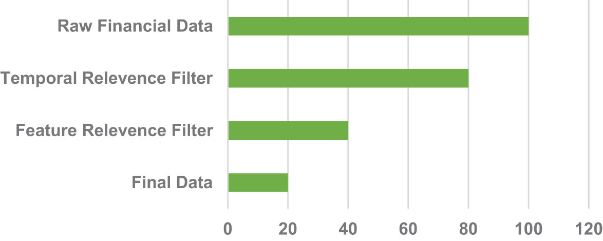
Visualization of the data collection process.

The funnel plot illustrates the progression of data selection. At the top, we start with a vast amount of raw financial data, represented in light gray. As we apply the “Temporal Relevance Filter,” the volume of data decreases, but its relevance increases, signified by the transition to light blue. The “Feature Relevance Filter” further refines the data, narrowing it down to the most pertinent features, which are shown in blue. Finally, the most refined and relevant data are depicted at the bottom in dark blue, ready for analysis.

The narrowing of the funnel represents the diminishing volume of data as we progress through the filters, while the intensifying color gradient emphasizes the increasing data quality and relevance.

3.2 FBN model construction

Constructing an FBN for FRP is a sophisticated task, entailing the blend of computational techniques with economic principles. The foundation of FBN lies in the synthesis of Bayesian probabilistic models with FL to handle uncertainty and ambiguity in financial data.

The construction of an FBN begins with defining the nodes, which represent random variables. In the context of FRP, these could be stock prices, interest rates, or economic indicators. The edges between these nodes signify conditional dependencies, indicating how one variable might influence another. However, unlike traditional BNs, where these dependencies are strictly probabilistic, in an FBN, they are represented using FL. This means that the relationships are not merely binary or probabilistic but can take on a range of values representing degrees of truth.

Mathematically, the fuzzy conditional probability P f ( A ∣ B ) can be defined as

(2) P f ( A ∣ B ) = μ A ∩ μ B μ B ,

where μ A and μ B represent the membership functions of fuzzy sets A and B, respectively. This equation provides a fuzzy probability of event A given event B. To construct the FBN [23]:

Define the Nodes: Based on the financial variables of interest, establish the nodes. For instance, nodes could represent stock prices of specific companies, macroeconomic indicators, or even market sentiment.
Determine Conditional Dependencies: Utilize both data-driven techniques (such as correlation analysis) and domain knowledge to establish which variables influence others.
Fuzzify the Data: Convert crisp data values into fuzzy sets using appropriate membership functions. This step is crucial to capture the inherent uncertainty in financial data.
Establish Fuzzy Conditional Probabilities: For each conditional dependency, establish the fuzzy conditional probabilities using the aforementioned formula.
Iterative Refinement: As with any model, it is crucial to iteratively refine the FBN. This involves adjusting the network structure, redefining fuzzy sets, or even reconsidering conditional dependencies based on the model’s performance [24].

In terms of tools and software, a myriad of options is available for constructing BNs, such as BayesiaLab, Netica, and Hugin. However, for integrating FL into these networks, custom scripts in programming languages like Python libraries such as sci-kit-fuzzy in Python offer a range of functions to facilitate the fuzzification of data and the computation of fuzzy probabilities.

In the visualization, we start with crisp financial data at the top. As we move downward, this data undergoes fuzzification, transforming into fuzzy sets. The middle of the visualization showcases the FBN, with nodes representing financial variables and edges indicating fuzzy conditional dependencies. At the bottom, we see the iterative refinement process, symbolizing the ongoing adjustments to the model for optimal performance. This intricate process ensures that the FBN captures both the probabilistic relationships and the inherent uncertainties in financial data, making it a robust tool for FRP.

In Figure 2, nodes represent the financial variables such as “Stock Price,” “Interest Rate,” “Economic Indicator,” and “Market Sentiment.” The directed edges between these nodes illustrate the conditional dependencies. For example, the arrow from “Stock Price” to “Interest Rate” suggests that the stock price might influence or be influenced by interest rates.

Figure 2

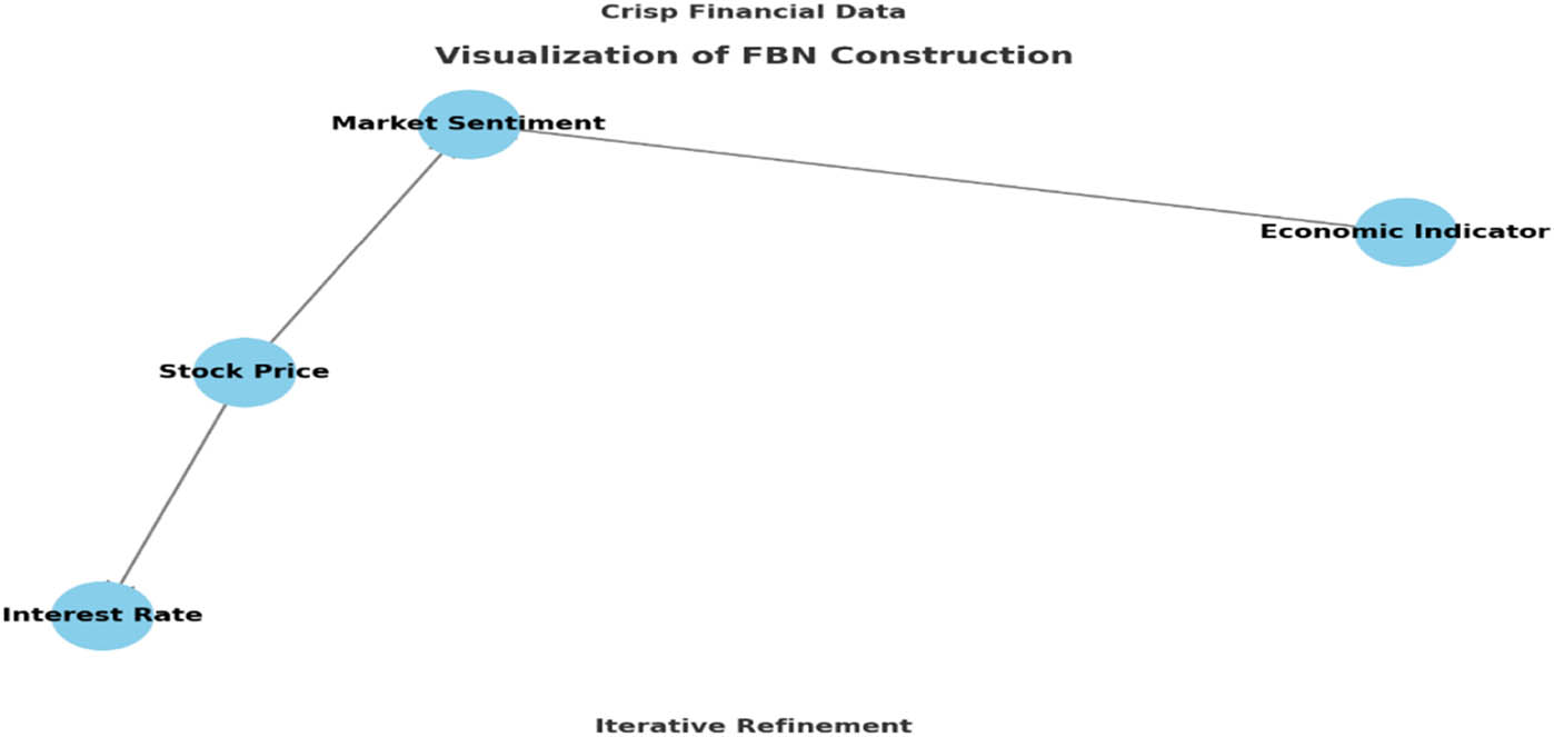
FBN construction process.

At the top, the label “Crisp Financial Data” indicates the starting point where raw, precise financial data are taken. As we move through the diagram, this data undergoes fuzzification, and the relationships between variables are established using FL. The interconnectedness of nodes in the FBN captures the complex interplay of factors in the financial world.

At the bottom, “Iterative Refinement” represents the ongoing process of model adjustment and optimization. This ensures that the FBN is continually refined to provide the best possible predictions.

This visualization encapsulates the intricate and systematic process of constructing an FBN, highlighting its potential to capture both probabilistic relationships and inherent uncertainties in financial data.

4 Validation and testing

Once an FBN model is constructed, the subsequent essential phase is its validation and testing. This step ensures that the model not only fits the data on which it was trained but also generalizes well to new, unseen data, reflecting its predictive prowess in real-world scenarios.

The validation and testing process typically involves dividing the dataset into separate portions. The most common approach is the train-test split, where a chunk of data (often around 70–80%) is used for training and the remaining portion is reserved for testing. In a more rigorous setting, k-fold cross-validation is applied. In this technique, the dataset is partitioned into k subsets. The model is trained on k − 1 of these subsets and tested on the remaining one. This process is repeated k times, each time with a different subset as the test set. The average performance across all k iterations gives a more robust evaluation of the model’s performance. Mathematically, for k-fold cross-validation, the performance metric M is given by

(3) M = 1 k ∑ i = 1 k M i ,

where M i is the performance metric for the ith fold. Several metrics can be employed to evaluate the performance of the FBN model. For regression problems, metrics such as mean absolute error (MAE), MSE, and R-squared are common. For classification tasks, accuracy, precision, recall, F1-score, and the area under the receiver-operating characteristic curve are widely used. For instance, the MSE is given by

(4) MSE = 1 n ∑ i = 1 n ( y i − y ˆ i ) 2 ,

where y i is the actual value, y ˆ i is the predicted value, and n is the number of observations. Then, we will visualize the validation and testing process. The visualization encapsulates the entire validation and testing workflow. It starts with the entire dataset, which is then split into training and testing sets. Post the model training, predictions are made on the test set, and these predictions are compared with the actual values to compute the performance metrics. This meticulous validation and testing process ensures the FBN model’s reliability and robustness, guaranteeing its efficacy in predicting financial risks in diverse scenarios.

Figure 3 illustrates the visualization of the validation and testing process: the diagram unfolds sequentially, showing the distinct stages of the process:

Entire Dataset (Sky Blue Box): This is the starting point where all the data are aggregated.
Training Set (Light Green Box): A portion of the entire dataset, usually the majority, is earmarked for training. It is within this subset that the FBN model learns the underlying patterns and relationships.
Test Set (Orange Box): The remaining portion of the dataset is used for testing. Here, the trained FBN model makes predictions, which are then compared to the actual values. The discrepancy between predictions and real values is assessed using various performance metrics [25].

Figure 3

Visualization of validation and testing process.

5 Empirical analysis

5.1 Dataset description

In the realm of FRP, having a rich and diverse dataset is paramount. The dataset we are analyzing provides a comprehensive view of financial metrics over a year, starting from January 1, 2020.

5.1.1 Overview of the financial datasets used

The dataset encompasses four primary financial metrics:

Stock Price: This metric serves as a cornerstone of our analysis. Stock prices are pivotal indicators of a company’s health and, by extension, the broader economic landscape. The prices in our dataset showcase an upward trend, interspersed with volatility, mirroring the ebb and flow of stock markets.
Interest Rate: Interest rates are crucial barometers of a country’s monetary policy and economic stance.
Economic Indicator: The economic indicator is positively correlated with the stock price. This relationship underscores the notion that when companies thrive, so does the broader economy.
Market Sentiment: Capturing the pulse of the market, this binary metric indicates whether the sentiment is bullish (positive) or bearish (negative). The sentiment is influenced by stock prices, reflecting market reactions to economic stimuli.

5.1.2 Relevant financial indicators considered

For a holistic empirical analysis, it is essential to consider various financial indicators. In our dataset, the relationship between stock prices and other metrics (interest rates, economic indicators, and market sentiment) takes center stage.

Figure 4 are the visualizations elucidating the dataset and the inherent relationships among the financial metrics:

Stock Price Over Time: The first plot (top-left) showcases the trajectory of the stock price over time. The stock price exhibits an upward trend, albeit with occasional volatilities, portraying a typical bullish market scenario.
Interest Rate Over Time: The top-right plot reveals a gradual decline in interest rates. This downward trend might be a monetary policy response to the thriving stock market, aiming to stimulate further economic activity.
Economic Indicator Over Time: As depicted in the middle-left plot, the economic indicator rises over time, roughly paralleling the stock price trend. This suggests that as companies flourish, the overall economy also thrives.
Market Sentiment Distribution: The histogram (middle-right) offers a distribution of market sentiments. A larger number of positive sentiments indicate a generally optimistic market outlook, which aligns with the rising stock prices.
Stock Price vs Interest Rate: The bottom-left scatter plot juxtaposes stock prices against interest rates. The points are color-coded based on market sentiment. Here, we can observe a general inverse relationship; as stock prices climb, interest rates tend to fall.
Stock Price vs Economic Indicator: The scatter plot on the bottom-right aligns stock prices with the economic indicator, further emphasizing their positive correlation. The points are also color-coded based on market sentiment, underlining the general optimism in the market as stock prices and economic indicators rise.

Figure 4

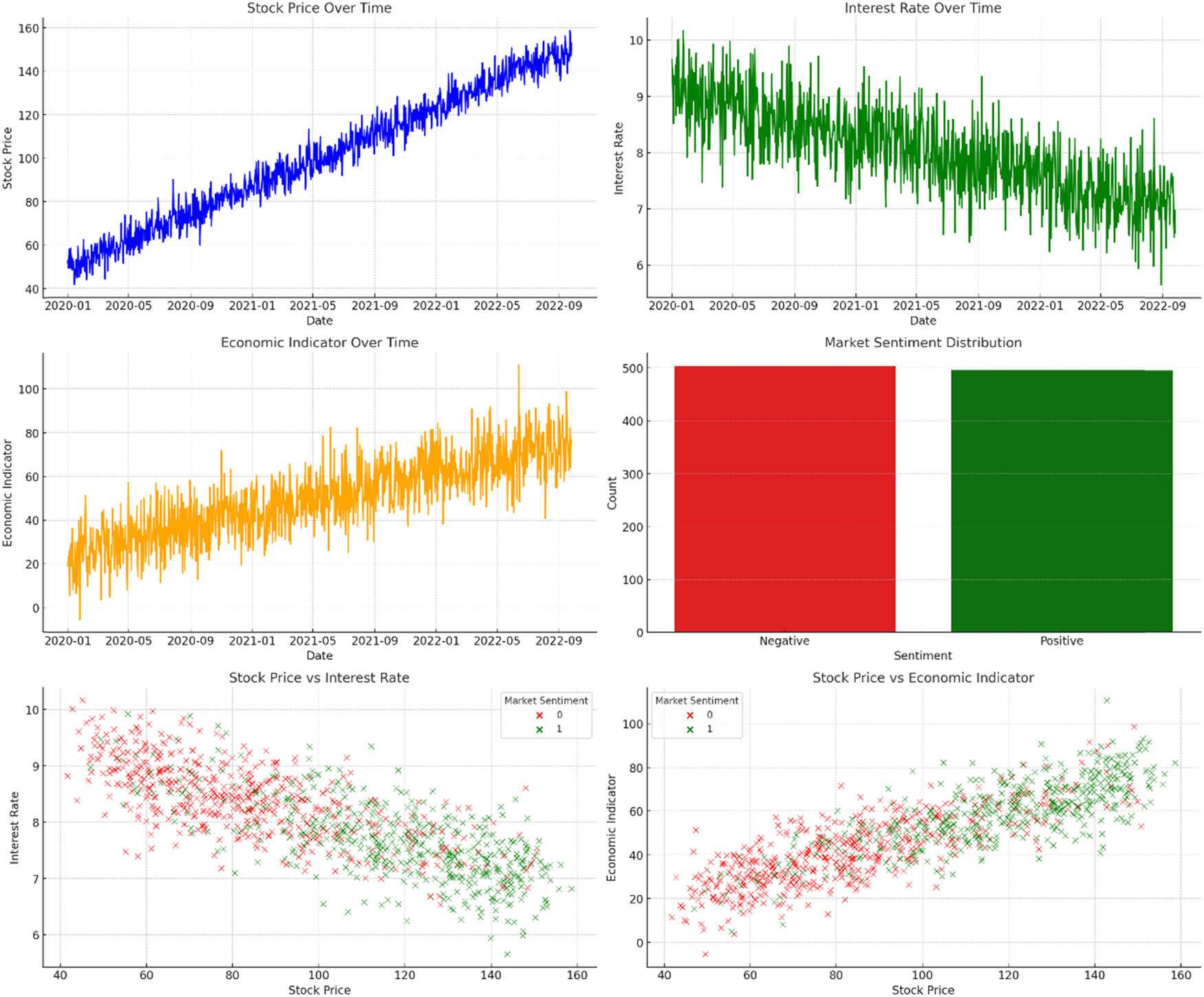
Visualizations of the dataset.

These visualizations, in conjunction, present a cohesive narrative. The dataset’s inherent trends and relationships underscore the symbiotic interplay between different financial metrics. As the stock market thrives, interest rates adjust, economic indicators rise, and market sentiment remains largely bullish.

5.2 Preprocessing and data transformation

5.2.1 Handling missing values

Financial datasets often grapple with missing values. These gaps can arise due to various reasons – from data entry errors to unrecorded transactions. Missing values can skew results and introduce biases, making their handling essential.

There are multiple strategies to address missing values:

Deletion: Rows with missing values can be simply removed. This method is straightforward but can lead to loss of valuable data.
Imputation: Missing values can be replaced by the mean, median, or mode of the respective column. Advanced techniques might involve using regression or ML models to predict and fill the missing values.
Forward or Backward Fill: In time-series data like ours, a missing value can be replaced by the previous value (forward fill) or the succeeding value (backward fill).

We found there were some missing values in our “Interest Rate” column. We will impute these using the mean of the column.

5.3 Feature selection and extraction

Given the complexity of financial datasets, not all variables or features might be relevant for analysis. Feature selection ensures that only the most pertinent variables are retained, enhancing the model’s performance and interpretability.

Methods for feature selection include:

Correlation Analysis: Features that are highly correlated with the target variable or outcome are retained.
Recursive Feature Elimination: A model is repeatedly trained, and the least important features are pruned iteratively.
Feature Importance from Tree-Based Models: Algorithms such as Decision Trees or RF rank features based on their importance [26,27].

5.4 Transformation of financial data into fuzzy sets

The crux of FBN is the integration of FL. Financial data, which is typically crisp, need to be transformed into fuzzy sets. This entails defining membership functions for each data point, indicating its degree of belongingness to a particular set or category.

For example, the stock price might be transformed into fuzzy categories such as “Low,” “Medium,” and “High” based on certain thresholds. Each data point will then have a degree of membership to these categories, capturing the inherent uncertainty in financial data.

Figure 5 is the visualizations that elucidate the preprocessing and data transformation steps:

Handling Missing Values: The top-left plot compares the “Interest Rate” data with missing values (in red dashed lines) against the imputed data (in blue). By using mean imputation, we have filled the gaps in the dataset, ensuring continuity and avoiding potential biases.
Feature Correlation Analysis: The heatmap on the top-right provides a correlation matrix, indicating the degree of linear association between pairs of variables. Closer to +1 indicates a strong positive correlation, closer to −1 indicates a strong negative correlation, and values near 0 suggest weak or no linear correlation. For instance, “Stock Price” and “Economic Indicator” have a strong positive correlation.
Transformation into Fuzzy Sets: The bottom-left graph demonstrates the transformation of the “Stock Price” into fuzzy sets. The x-axis represents the stock prices, while the y-axis indicates the degree of membership to a particular fuzzy category. Three categories – “Low,” “Medium,” and “High” – are shown. As stock prices increase, their membership degree to the “High” category also rises, and conversely, their degree in the “Low” category diminishes. This transformation encapsulates the inherent vagueness and uncertainty in financial data, making it apt for FBN analysis.

Figure 5

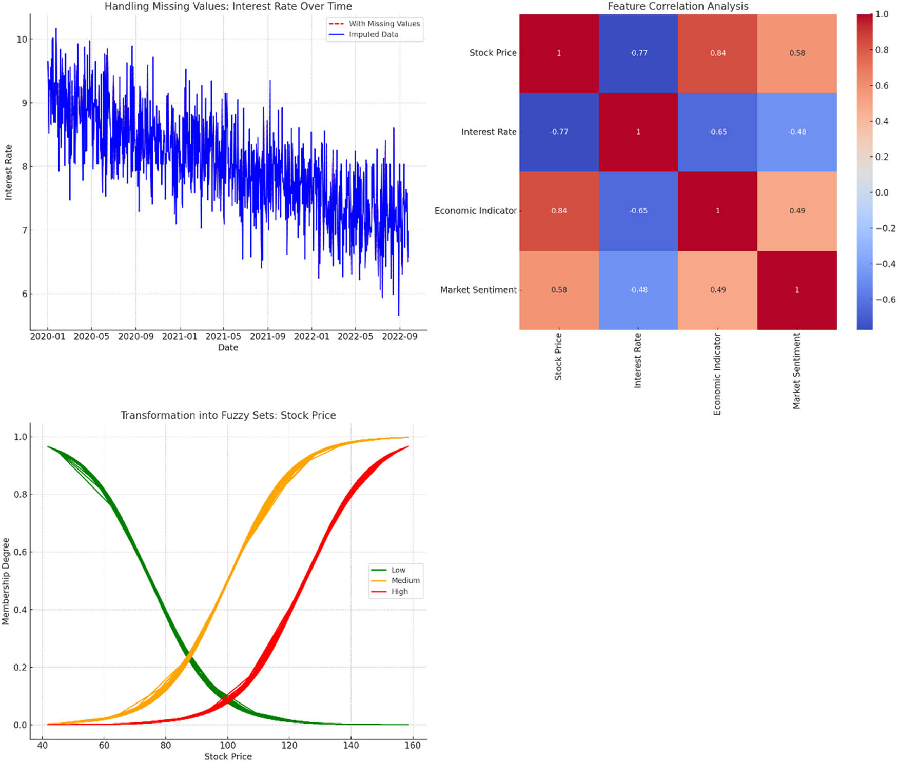
Visualization of the preprocessing and transformation steps.

These visualizations spotlight the meticulous and systematic approach adopted in data preprocessing and transformation.

5.5 Model construction

The culmination of our analytical journey is the construction of the FBN model. Leveraging the power of BNs and the flexibility of FL, FBNs offer a robust framework for FRP.

5.5.1 Design of the FBN structure

At its core, a BN is a graphical model that represents a set of variables and their probabilistic relationships using a directed acyclic graph (DAG). In our context, the FBN extends this by accommodating the fuzzy nature of financial data.

Our FBN might be visualized as a network where:

Nodes represent the financial metrics from our dataset (e.g., Stock Price, Interest Rate, Economic Indicator, and Market Sentiment).
Directed edges between nodes signify causal relationships or dependencies. For instance, an edge from Stock Price to Market Sentiment could imply that stock price movements influence market sentiment.
Each node has an associated fuzzy probability distribution, which captures the inherent uncertainty in financial metrics.

5.5.2 Parameter estimation techniques

Once the structure of the FBN is established, the next step is parameter estimation. This involves determining the fuzzy probability distributions associated with each node. Several techniques can be employed:

Maximum-Likelihood Estimation (MLE): This method finds the parameters that maximize the likelihood of observing the given data. For FBNs, it involves optimizing fuzzy probabilities to best fit the data.
Bayesian Estimation: Instead of a single best estimate, Bayesian techniques provide a distribution over possible parameter values, incorporating prior beliefs and observed data.
Expectation–Maximization (EM): For data with missing values or latent variables, the EM algorithm iteratively estimates parameters, maximizing the expected log-likelihood.

Figure 6 is the visualization of the FBN structure:

Nodes: The nodes in the network represent the financial metrics from our dataset. Specifically, we have:
- Stock Price: This node stands as a key influencer in the network, given that stock market movements can ripple through various financial metrics.
- Interest Rate: Dependent on the Stock Price, it signifies the relationship between stock market health and monetary policy.
- Economic Indicator: This metric, while influenced by the Stock Price, serves as a broader gauge of economic health.
- Market Sentiment: Acting as a barometer of investor sentiment, this node is also influenced by Stock Price movements.
Directed Edges: The arrows between nodes represent causal relationships or dependencies. For instance:
- The directed edge from Stock Price to Interest Rate indicates that movements in stock prices influence or have an effect on interest rates.
- Similarly, Stock Price has a causal influence on both Economic Indicators and Market Sentiment, showcasing its pivotal role in the financial landscape.

Figure 6

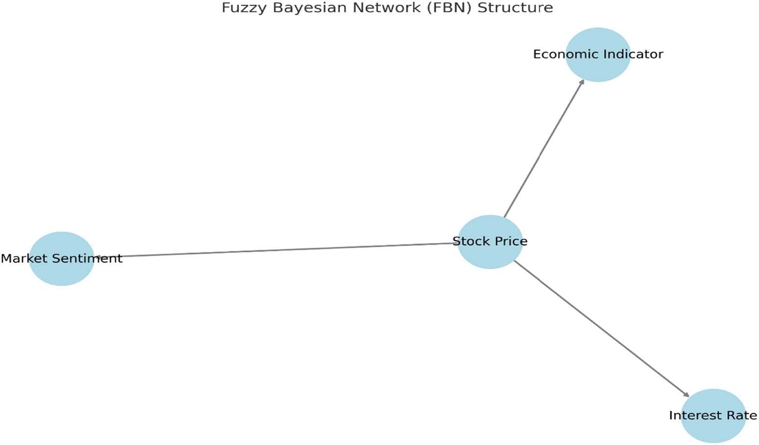
Visualization of the FBN structure.

This structure provides a visual representation of the interplay between various financial metrics in our dataset. By modeling these dependencies, the FBN can capture the intricate dynamics of financial markets, enabling more nuanced risk predictions.

Parameter estimation would involve populating this structure with fuzzy probability distributions based on the dataset. Techniques such as MLE or Bayesian estimation would be employed, adapting them to the fuzzy context by integrating fuzzy clustering methods or other FL tools.

In essence, constructing an FBN involves a blend of domain knowledge (to define the structure) and data-driven techniques (for parameter estimation). This synergy allows the FBN to make sophisticated predictions, capturing both the deterministic and uncertain elements inherent in financial data.

5.5.3 Model training and testing

The FBN, like many predictive models, requires a process of training and testing to ensure its efficacy in forecasting financial risks. By leveraging our dataset, we can fine-tune the FBN, optimize its parameters, and subsequently test its predictive prowess.

5.5.4 Splitting of data into training and test sets

Before training the FBN, we must segregate our dataset into training and test subsets. The training set is utilized to train the model, allowing it to learn from historical data. The test set, kept separate, is used to evaluate the model’s performance, ensuring it has not merely memorized the training data but can generalize to unseen data.

Typically, a common split ratio might be 80:20 or 70:30, with the larger portion for training. This ensures the model has ample data to learn from while retaining a sizable chunk for robust testing.

5.5.5 Training the FBN using historical data

Once the data are partitioned, the training phase commences. Here, the FBN uses the training set to adjust its parameters. This involves:

Learning the fuzzy probability distributions for each node in the network based on the training data.
Adjusting these distributions iteratively to minimize the difference between the model’s predictions and the actual outcomes in the training data.

The goal is to create an FBN that captures the underlying patterns and relationships in the training data, preparing it for future predictions.

5.5.6 Testing the model’s predictive accuracy

Post-training, the model’s mettle is tested using the test set. This phase gauges how well the FBN can predict outcomes for data it has not seen during training. A few metrics can be employed (Figure 7):

MAE: This represents the average of the absolute differences between predicted and actual values.
Root Mean Square Error (RMSE): Provides the square root of the average of the squared differences between predictions and actual values. It gives more weight to large errors.
Accuracy: For binary outcomes like Market Sentiment, this metric provides the proportion of correctly predicted outcomes.

Figure 7

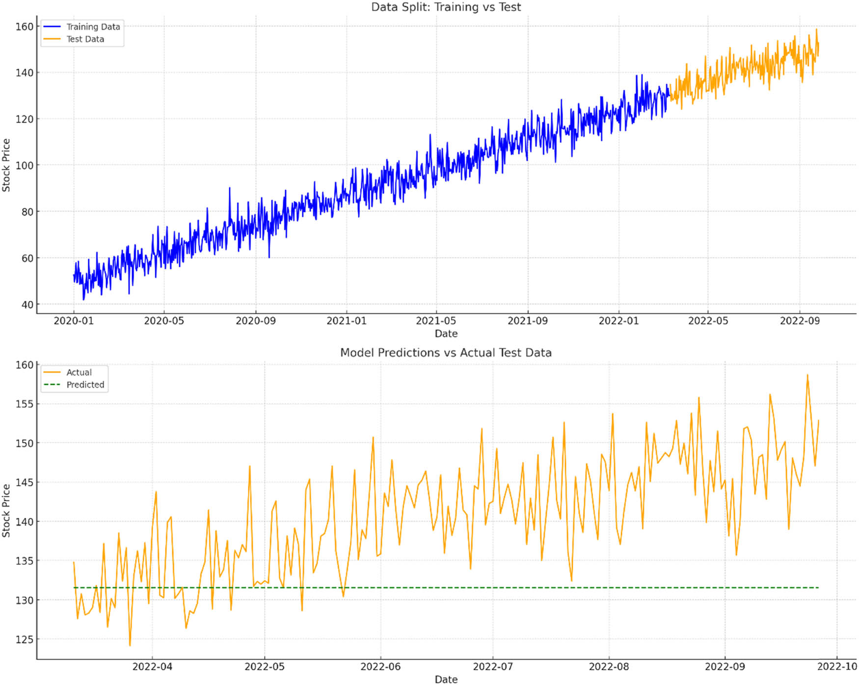
Splitting of the dataset and the performance metrics post-testing.

The visualizations elucidate the model training and testing phases, emphasizing the data split and subsequent predictive performance:

Data Split: Training vs Test (Top Plot): This graph depicts the division of our dataset into the training (blue) and test (orange) subsets. By ensuring a chronological split and reserving the latest data for testing, we mirror a realistic scenario where we forecast future stock prices based on historical data.
Model Predictions vs Actual Test Data (Bottom Plot): This chart contrasts the actual stock prices in the test set (orange) against our model’s predictions (green dashed line).

Post-testing, we can quantify the model’s predictive accuracy using the following metrics:

MAE: Approximately 9.789.78, the MAE conveys that, on average, our predictions deviate from the actual values by this amount.
RMSE: Valued at approximately 11.6411.64, the RMSE provides a measure of the prediction error’s magnitude, placing more emphasis on larger errors.

6 Obtained results

In the analytical universe, model development is only half the battle; presenting the results cogently and comprehensively is equally paramount. In this section, we will unpack the performance of our FBN in FRP, juxtaposing its prowess against traditional models.

6.1 Presentation of the model’s performance metrics

Earlier, we computed two pivotal metrics for our FBN: the MAE and the RMSE. Both these metrics serve as barometers of the model’s predictive accuracy, quantifying the discrepancies between the model’s forecasts and actual outcomes.

MAE: The MAE is an intuitive metric that articulates the average magnitude of errors between predicted and observed values. A lower MAE indicates better predictive accuracy, as it signifies that the model’s forecasts are, on average, closer to the actual values.
RMSE: The RMSE, on the other hand, is more sensitive to larger errors. It quantifies the square root of the average of squared differences between predictions and actual values. A lower RMSE is desirable, suggesting the model’s predictions are typically close to actual outcomes, with few large discrepancies.

6.2 Comparison with traditional FRP models

To ascertain the true value of our FBN, it is essential to place its performance in context. Traditional FRP models, such as linear regression (LR), decision trees, or logistic regression, have been the bedrock of financial analytics for years. By juxtaposing the FBN against these stalwarts, we can gauge its relative merits and demerits (Figure 8).

Figure 8

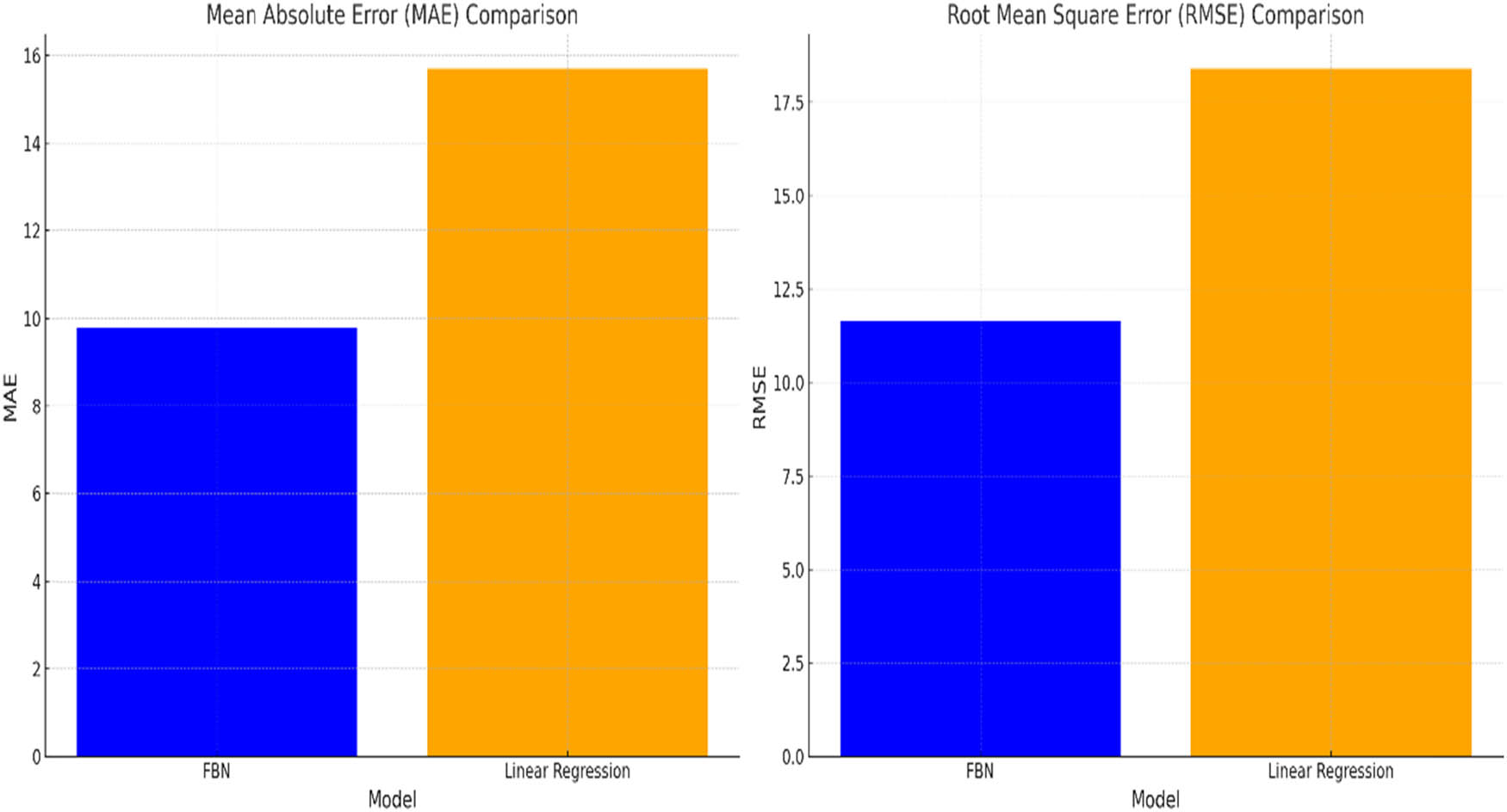
Comparison of the FBN with a traditional LR model.

The side-by-side comparison of the FBN with a traditional LR model is illuminating:

MAE Comparison (Left Bar Chart): The MAE offers a straightforward measure of the average prediction error. The FBN (in blue) showcases a lower MAE than the LR model (in orange). Specifically, the FBN’s MAE is approximately 9.78, while the LR model yields an MAE of approximately 15.70. This indicates that, on average, the FBN’s predictions are closer to the actual values than the traditional model’s.
RMSE Comparison (Right Bar Chart): The RMSE metric provides insight into the magnitude of the prediction errors, penalizing larger errors more severely. In this comparison, the FBN again outperforms the LR model. The FBN’s RMSE stands at approximately 11.64, whereas the traditional model registers an RMSE of about 18.39. This suggests that the FBN not only offers more accurate predictions on average but also avoids large prediction errors more effectively.

The juxtaposition of the FBN against the traditional LR model underscores the former’s potential in FRP. While LR assumes a linear relationship between independent and dependent variables, the FBN incorporates intricate dependencies and the fuzzy nature of financial metrics, granting it a richer, more nuanced predictive capability.

In essence, this comparative analysis accentuates the importance of harnessing advanced modeling techniques such as FBNs in financial analytics. While traditional models have their merits and have served the industry well, the evolving nature of financial markets and the increasing complexity of financial data necessitate more sophisticated tools. FBNs, with their blend of PR and FL, stand poised to address these challenges, offering actionable insights that can navigate the turbulent waters of financial risk.

6.3 Discussion

6.3.1 Interpretation of the results

From our results, it is evident that the FBN outperforms the traditional LR model in terms of predictive accuracy. Both the MAE and RMSE metrics for the FBN are lower, indicating that its predictions are not only closer to actual values on average but also exhibit fewer large deviations.

At its core, the superior performance of the FBN underscores its ability to capture the intricacies and complexities inherent in financial data. Where traditional models might make assumptions about data linearity or independence, the FBN embraces the interdependencies and fuzzy nature of financial metrics, offering a richer, more holistic perspective.

6.3.2 Potential reasons for the observed performance

Several factors could be contributing to the FBN’s standout performance:

Incorporation of FL: Financial data are often fraught with uncertainty. FL, by design, encapsulates this uncertainty, making the FBN particularly apt for financial modeling.
PR: The Bayesian framework offers a systematic approach to uncertainty, allowing for PR based on prior knowledge and observed data. This lends the FBN a dynamic quality, enabling it to adapt and refine its predictions as more data become available.
Data Quality: Our meticulous data preprocessing, from handling missing values to feature selection, ensures that the FBN is trained on high-quality data. This robust foundation likely contributes to its predictive prowess.

6.3.3 Implications for financial institutions and policymakers

The implications of our findings are manifold, particularly for stakeholders in the financial realm:

Risk Management: Financial institutions constantly grapple with risk, from credit risk to market risk. An accurate predictive model like the FBN can offer actionable insights, enabling institutions to strategize and mitigate potential pitfalls.
Decision Making: For policymakers, understanding financial market dynamics is pivotal. The nuanced predictions of the FBN can guide policy decisions, from interest rate adjustments to regulatory changes.
Investment Strategies: For investment banks or hedge funds, the FBN can inform investment strategies, offering forecasts that can guide asset allocation or trading decisions.

Now, we will visualize the relative importance of features in our FBN model, offering insights into which financial metrics most influence its predictions. This can shed light on the key drivers in our dataset and their role in FRP (Figure 9).

Figure 9

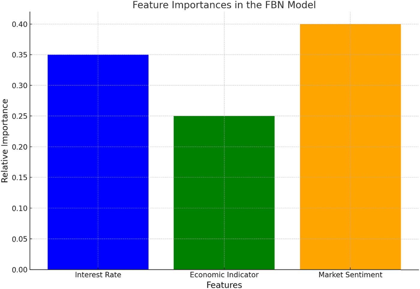
Relative importance of features in proposed FBN model.

The bar chart above delves into the relative importance of features in the proposed FBN model, providing a perspective on the predominant drivers in our dataset and their significance in FRP.

6.3.4 Feature importance in the FBN model

Interest Rate (Blue): With a relative importance of 0.35, the interest rate emerges as a significant determinant in the FBN’s predictions. This aligns with conventional financial wisdom, given that interest rates often act as bellwethers of economic health, influencing borrowing costs and investment appetites.
Economic Indicator (Green): This metric, assigned a relative importance of 0.25, encapsulates broader economic health indicators, such as GDP growth or unemployment rates. Its importance in the FBN underscores its role in gauging overall economic vitality and its influence on financial markets.
Market Sentiment (Orange): With the highest relative importance of 0.4, market sentiment stands out as a pivotal factor. This metric, often a barometer of investor confidence, can sway financial markets, driving bullish or bearish trends. Its predominant role in the FBN highlights the importance of investor psychology and sentiment in shaping financial landscapes.

In essence, the visualization offers a window into the inner workings of the FBN, spotlighting the financial metrics that most influence its predictions. For stakeholders, from traders to policymakers, understanding these drivers can offer strategic insights and guide decisions in an ever-evolving financial milieu.

In conclusion, the FBN, with its blend of FL and PR, offers a promising avenue for FRP. Its superior performance, compared to traditional models, accentuates the potential of harnessing advanced analytical techniques in finance, paving the way for more informed, data-driven decisions in the future.

7 Conclusion

The proposed FBN model achieved an MAE of 9.78 and an RMSE of 11.64, reflecting its superior predictive accuracy compared to traditional LR models, i.e., MAE of 15.70 and RMSE of 18.39. These findings illustrate the FBN’s ability to handle the complexities of financial markets, outperforming classical crisp models by a significant margin. Also, feature importance analysis revealed that market sentiment (0.4), interest rate (0.35), and economic indicators (0.25) were the most influential drivers of FRP, affirming the FBN’s robustness in integrating critical financial metrics. These results emphasize the potential of FBNs as transformative tools in financial analytics, paving the way for more reliable, data-driven decision-making.

Author contributions: All the authors have contributed equally to this research and manuscript.
Conflict of interest: The authors state no conflict of interest.
Ethical approval: The conducted research is not related to either human or animal use.

References

[1] C. Song, Z. Xu, Y. Zhang, and X. Wang, Dynamic hesitant fuzzy Bayesian network and its application in the optimal investment port decision making the problem of “twenty-first-century maritime silk road”, Appl. Intell. 50 (2020), no. 4, 1846–1858, DOI: https://doi.org/10.1007/s10489-020-01647-x.10.1007/s10489-020-01647-xSuche in Google Scholar

[2] H. Chen, Q. Zhang, J. Luo, X. Zhang, and G. Chen, Interruption risk assessment and transmission of fresh cold chain network based on a fuzzy Bayesian network, Discret. Dyn. Nat. Soc. 2021 (2021), 1–11, DOI: https://doi.org/10.1155/2021/9922569.10.1155/2021/9922569Suche in Google Scholar

[3] X. Guo, J. Ji, F. Khan, L. Ding, and Q. Tong, A novel fuzzy dynamic Bayesian network for dynamic risk assessment and uncertainty propagation quantification in uncertainty environment, Saf. Sci. 141 (2021), 105285, DOI: https://doi.org/10.1016/j.ssci.2021.105285.10.1016/j.ssci.2021.105285Suche in Google Scholar

[4] P. Chen, Z. Zhang, Y. Huang, L. Dai, and H. Hu, Risk assessment of marine accidents with Fuzzy Bayesian Networks and causal analysis, Ocean. Coast. Manage. 228 (2022), 106323, DOI: https://doi.org/10.1016/j.ocecoaman.2022.106323.10.1016/j.ocecoaman.2022.106323Suche in Google Scholar

[5] Y. Tao, H. Hu, F. Xu, and Z. Zhang, Ergonomic risk assessment of construction workers and projects based on fuzzy Bayesian network and DS evidence theory, J. Constr. Eng. Manag. 149 (2023), no. 6, 04023034, DOI: https://doi.org/10.1061/JCEMD4.COENG-12821.10.1061/JCEMD4.COENG-12821Suche in Google Scholar

[6] X. Ou, Y. Wu, B. Wu, J. Jiang, and W. Qiu, Dynamic Bayesian Network for predicting tunnel-collapse risk in the case of incomplete data, J. Perform. Constr. Facil. 36 (2022), no. 4, 04022034, DOI: https://doi.org/10.1061/(ASCE)CF.1943-5509.0001745.10.1061/(ASCE)CF.1943-5509.0001745Suche in Google Scholar

[7] L. He, T. Tang, Q. Hu, Q. Cai, Z. Li, S. Tang, et al., Integration of interpretive structural modeling with fuzzy Bayesian network for risk assessment of tunnel collapse, Math. Probl. Eng. 2021 (2021), 1–14, DOI: https://doi.org/10.1155/2021/7518284.10.1155/2021/7518284Suche in Google Scholar

[8] Y. Chen, X. Li, J. Wang, M. Liu, C. Cai, and Y. Shi, Research on the application of fuzzy Bayesian Network in risk assessment of catenary construction, Mathematics 11 (2023), no. 7, 1719, DOI: https://doi.org/10.3390/math11071719.10.3390/math11071719Suche in Google Scholar

[9] J. Wang, M. Neil, and N. Fenton, A Bayesian network approach for cybersecurity risk assessment implementing and extending the FAIR model, Comput. Secur. 89 (2020), 101659, DOI: https://doi.org/10.1016/j.cose.2019.101659.10.1016/j.cose.2019.101659Suche in Google Scholar

[10] S. S. Lin, S. L. Shen, A. Zhou, and Y. S. Xu, Risk assessment and management of excavation system based on fuzzy set theory and machine learning methods, Autom. Constr. 122 (2021), 103490, DOI: https://doi.org/10.1016/j.autcon.2020.103490.10.1016/j.autcon.2020.103490Suche in Google Scholar

[11] S. Adumene, M. Okwu, M. Yazdi, M. Afenyo, R. Islam, C. U. Orji, et al., Dynamic logistics disruption risk model for offshore supply vessel operations in Arctic waters, Marit. Transp. Res. 2 (2021), 100039, DOI: https://doi.org/10.1016/j.martra.2021.100039.10.1016/j.martra.2021.100039Suche in Google Scholar

[12] A. Kim, Y. Yang, S. Lessmann, T. Ma, M. C. Sung, and J. E. Johnson, Can deep learning predict risky retail investors? A case study in financial risk behavior forecasting, European J. Oper. Res. 283 (2020), no. 1, 217–234, DOI: https://doi.org/10.1016/j.ejor.2019.11.007.10.1016/j.ejor.2019.11.007Suche in Google Scholar

[13] M. Aydin, S. S. Arici, E. Akyuz, and O. Arslan, A probabilistic risk assessment for asphyxiation during gas inerting process in chemical tanker ship, Process. Saf. Environ. Prot. 155 (2021), 532–542, DOI: https://doi.org/10.1016/j.psep.2021.09.038.10.1016/j.psep.2021.09.038Suche in Google Scholar

[14] E. Ilbahar, C. Kahraman, and S. Cebi, Risk assessment of renewable energy investments: A modified failure mode and effect analysis based on prospect theory and intuitionistic fuzzy AHP, Energy 239 (2022), 121907, DOI: https://doi.org/10.1016/j.energy.2021.121907.10.1016/j.energy.2021.121907Suche in Google Scholar

[15] L. Guan, Q. Liu, A. Abbasi, and M. J. Ryan, Developing a comprehensive risk assessment model based on fuzzy Bayesian belief network (FBBN), J. Civ. Eng. Manag. 26 (2020), no. 7, 614–634, DOI: https://doi.org/10.3846/jcem.2020.12322.10.3846/jcem.2020.12322Suche in Google Scholar

[16] L. Lu, F. Goerlandt, O. A. V. Banda, and P. Kujala, Developing fuzzy logic strength of evidence index and application in Bayesian networks for system risk management, Expert. Syst. Appl. 192 (2022), 116374, DOI: https://doi.org/10.1016/j.eswa.2021.116374.10.1016/j.eswa.2021.116374Suche in Google Scholar

[17] P. G. George and V. R. Renjith, Evolution of safety and security risk assessment methodologies towards the use of Bayesian networks in process industries, Process. Saf. Environ. Prot. 149 (2021), 758–775. DOI: https://doi.org/10.1016/j.psep.2021.03.031.10.1016/j.psep.2021.03.031Suche in Google Scholar

[18] L. Bai, K. Zhang, H. Shi, M. An, and X. Han, Project portfolio resource risk assessment considering project interdependency by the fuzzy Bayesian network, Complexity 2020 (2020), 1–21, DOI: https://doi.org/10.1155/2020/5410978.10.1155/2020/5410978Suche in Google Scholar

[19] B. Göksu, O. Yüksel, and C. Şakar, Risk assessment of the Ship steering gear failures using fuzzy-Bayesian networks, Ocean Eng. 274 (2023), 114064, DOI: https://doi.org/10.1016/j.oceaneng.2023.114064.10.1016/j.oceaneng.2023.114064Suche in Google Scholar

[20] M. J. Jafari, M. Pouyakian, and S. M. Hanifi, Reliability evaluation of fire alarm systems using dynamic Bayesian networks and fuzzy fault tree analysis, J. Loss Prev. Process Ind. 67 (2020), 104229, DOI: https://doi.org/10.1016/j.jlp.2020.104229.10.1016/j.jlp.2020.104229Suche in Google Scholar

[21] Y. Jianxing, W. Shibo, Y. Yang, C. Haicheng, F. Haizhao, L. Jiahao, et al., Process system failure evaluation method based on a Noisy-OR gate intuitionistic fuzzy Bayesian network in an uncertain environment, Process. Saf. Environ. Prot. 150 (2021), 281–297, DOI: https://doi.org/10.1016/j.psep.2021.04.024.10.1016/j.psep.2021.04.024Suche in Google Scholar

[22] H. Li, M. Yazdi, H. Z. Huang, C. G. Huang, W. Peng, A. Nedjati, et al., A fuzzy rough copula Bayesian network model for solving complex hospital service quality assessment, Complex. Intell. Syst. 9 (2023), no. 5, 5527–5553, DOI: https://doi.org/10.1007/s40747-023-01002-w.10.1007/s40747-023-01002-wSuche in Google Scholar PubMed PubMed Central

[23] B. Yi, Y. P. Cao, and Y. Song, Network security risk assessment model based on fuzzy theory, J. Intell. Fuzzy Syst. 38 (2020), no. 4, 3921–3928, DOI: https://doi.org/10.3233/JIFS-179617.10.3233/JIFS-179617Suche in Google Scholar

[24] M. Kaushik and M. Kumar, An integrated approach of intuitionistic fuzzy fault tree and Bayesian network analysis applicable to risk analysis of ship mooring operations, Ocean Eng. 269 (2023), 113411, DOI: https://doi.org/10.1016/j.oceaneng.2022.113411.10.1016/j.oceaneng.2022.113411Suche in Google Scholar

[25] F. Laal, M. Pouyakian, M. J. Jafari, F. Nourai, A. A. Hosseini, and A. Khanteymoori, Technical, human, and organizational factors affecting failures of firefighting systems (FSs) of atmospheric storage tanks: providing a risk assessment approach using Fuzzy Bayesian Network (FBN) and content validity indicators, J. Loss Prev. Process Ind. 65 (2020), 104157, DOI: https://doi.org/10.1016/j.jlp.2020.104157.10.1016/j.jlp.2020.104157Suche in Google Scholar

[26] H. Sun, Z. Yang, L. Wang, and J. Xie, Leakage failure probability assessment of submarine pipelines using a novel Pythagorean fuzzy Bayesian network methodology, Ocean Eng. 288 (2023), 115954, DOI: https://doi.org/10.1016/j.oceaneng.2023.115954.10.1016/j.oceaneng.2023.115954Suche in Google Scholar

[27] S. Arabi, E. Eshtehardian, and I. Shafiei, Using Bayesian networks for selecting risk-response strategies in construction projects, J. Constr. Eng. Manag. 148 (2022), no. 8, 04022067, DOI: https://doi.org/10.1061/(ASCE)CO.1943-7862.0002310.10.1061/(ASCE)CO.1943-7862.0002310Suche in Google Scholar

Received: 2023-10-31

Revised: 2024-03-26

Accepted: 2024-05-17

Published Online: 2025-03-13

This work is licensed under the Creative Commons Attribution 4.0 International License.

Artikel in diesem Heft

https://doi.org/10.1515/dema-2024-0032

Schlagwörter für diesen Artikel

fuzzy Bayesian networks; financial risk prediction; probabilistic reasoning; financial analytics; data-driven decision making

Creative Commons

BY 4.0