On inequalities involving n-polynomial exponential-type convex functions
-
Muhammad Samraiz
 and
Yasser Elmasry
and
Yasser Elmasry

Abstract
This article deals with new generalized and more refined classes of Hermite-Hadamard and Fejér Hermite-Hadamard-type inequalities via
1 Introduction
The concept of convexity holds a significant value in mathematical areas. It describes the property of a function wherein the graph of a line segment joining any two points is located above the graph between the two points. While the primary source of convexity lies in geometry, it also possesses numerous useful qualities that render it applicable in a variety of scientific and mathematical domains. Convexity plays a helpful role in optimization problems [1], as well as in exploring other fields of study such as finance [2], machine learning [3,4], data science [5,6], control theory [7], and linear programming [8]. Furthermore, convexity is applied for the development of statistical models and efficient estimates [9,10].
The study of inequalities is essential in mathematics for resolving different types of problems. The necessity for inequalities arises since not all mathematical expressions are in the form of equality. Several kinds of inequalities exist in the literature, which include linear inequalities, quadratic inequalities, and rational inequalities. Some widely used inequalities include the triangle inequality [11,12], the inequality of arithmetic and geometric means [13,14], Jensen’s inequality [15,16], Bell’s inequality [17,18], and the Cauchy-Schwarz inequality [19,20]. Inequalities are extensively utilized in different mathematical branches such as analysis [21,22], number theory [23], and other scientific fields like engineering [24], economics [25], environmental science [26], and operation research [27]. Inequalities are also relevant to the field of convexity, especially in optimization theory. There are important convex inequalities in the literature, like the Jensen inequality, the Hermite-Hadamard inequality [28–30], and the Fejér-type inequality [31]. The widely known Hermite-Hadamard inequality, named after Charles Hermite and Jacques Hadamard,is defined as follows:
If
Due to important properties and usefulness of the Hermite-Hadamard inequality, many novel and generalized forms of Hermite-Hadamard-type inequality are being explored by researchers. Some of its refinements include its generalized forms to
where
In this article, we investigate a new generalized class of Hermite-Hadamard inequalities via
Definition 1
A function
for all
Definition 2
A function
where
The
Definition 3
A function
where
Now, we present the definition of the
Definition 4
[33] A function
holds for all
Theorem 1
(Hölder’s integral inequality [34]). Let f and g be the real-valued functions defined on the domain
where
Theorem 2
(Power-mean integral inequality [34]). Let f and g be the real-valued functions defined on the domain
The following Hölder-İscan inequality is the refined form of Hölder’s inequality.
Theorem 3
[35] Let f and g be the real-valued mappings defined on the domain
where
The following theorem presents an improved form of the power-mean integral inequality.
Theorem 4
[36] Let f and g be the real-valued mappings on the interval
where
Now, we present the following useful lemma which was proved by İscan.
Lemma 1
[37] Let the function
Studying generalized versions of inequalities allows for broader applicability and flexibility in various mathematical and scientific areas. It often leads to the discovery of new results and applications. Keeping in view the importance and extensive use of Hermite-Hadamard and Fejér Hermite-Hadamard in analysis and convexity theory, the present study is to explore generalized and refined Hermite-Hadamard inequalities via
2 Main results
In this section, we study some new generalized inequalities of Hermite-Hadamard type for
Theorem 5
Let
holds for
Proof
By applying Lemma 1, we obtain
By using Hölder’s inequality, we obtain
Since
Now, using the facts that
Hence, the required result is proved.□
Example 1
Here, we present the graphical representation to show the validity of Theorem 5. For this purpose, we make substitution
By choosing the parameters
Figure 1 shows the validity of inequality (2) for the above functions with
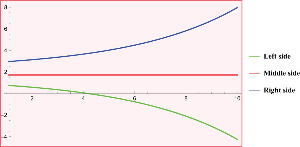
2D graph exhibiting inequality (2) for
In Table 1, a comparative analysis is provided for the functions
Comparison of the results between the double inequality in Example 1
| Functions | 1.1 | 2 | 4 | 6 | 8 | 10 |
|---|---|---|---|---|---|---|
|
|
0.76302 | 0.58126 | 0.06271 |
|
|
|
|
|
1.71828 | 1.71828 | 1.71828 | 1.71828 | 1.71828 | 1.71828 |
|
|
2.95526 | 3.13702 | 3.65557 | 4.48525 | 5.81887 | 7.97154 |
Now, for 3D representation, we choose
Figure 2 indicates the validity of inequality (2) with the choice of the parameters
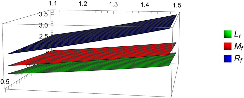
3D graph exhibiting inequality (3) for
Corollary 1
If we apply n-polynomial exponential-type convexity of
Corollary 2
If we specify
Theorem 6
Let the function
is true.
Proof
By utilizing Lemma 1 and then power mean inequality, we obtain
Since
Now, using the facts that
This proves the desired result.□
Example 2
Here, we present the graphical representation to show the validity of Theorem 6. For this purpose, we make substitution
Now, choosing the parameters
Figure 3 shows the validity of inequality (5) for the above functions with
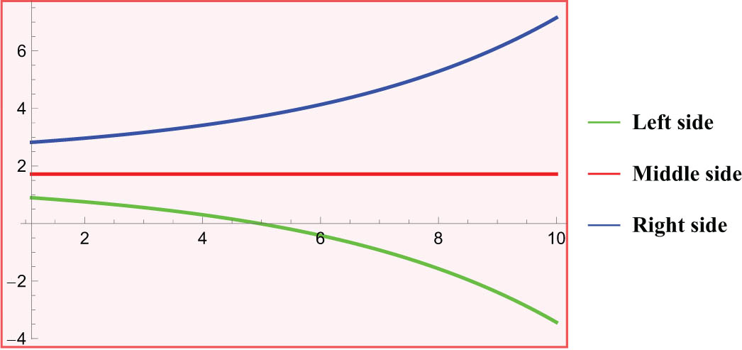
2D graph exhibiting inequality (5) for
In Table 2, a comparative analysis is provided for the functions
Comparison of the results between the double inequality in Example 2
| Functions | 1.1 | 2 | 4 | 6 | 8 | 10 |
|---|---|---|---|---|---|---|
|
|
0.90997 | 0.75257 | 0.30354 |
|
|
|
|
|
1.71828 | 1.71828 | 1.71828 | 1.71828 | 1.71828 | 1.71828 |
|
|
2.80831 | 2.96571 | 3.41474 | 4.13319 | 5.28804 | 7.15212 |
Now, for 3D representation, we chose
Figure 4 indicates the validity of inequality (6) with the choice of the parameters
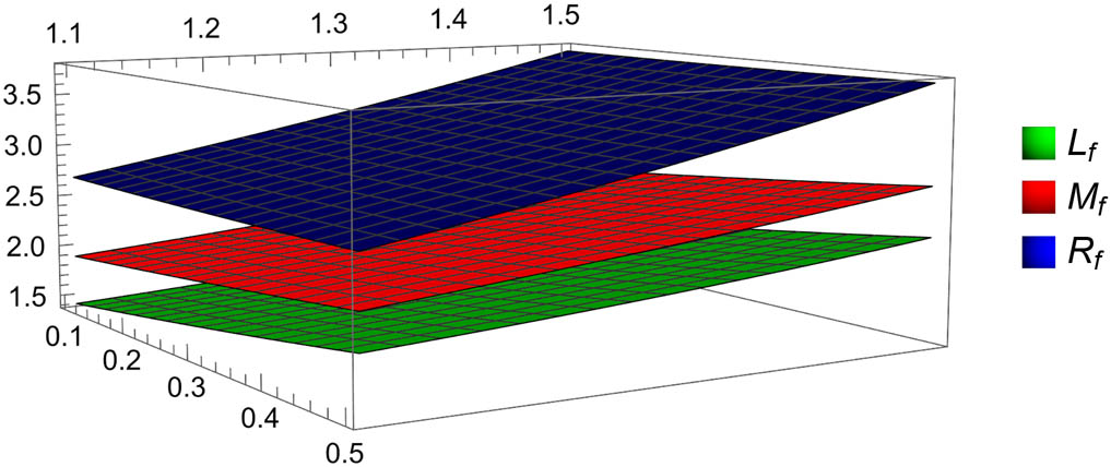
3D graph exhibiting inequality (6) for
Corollary 3
If n-polynomial exponential-type convexity of
Corollary 4
If we specify
Theorem 7
Let the mapping
is satisfied, where
Proof
If we apply the Hölder-İscan inequality upon Lemma 1 and then use the same steps as in Theorem 5, we arrive at inequality (7) which is the same as inequality (1).□
Theorem 8
Let the mapping
is true for
Proof
If we apply the improved power-mean inequality upon Lemma 1 and then use the same steps as in Theorem 6, we arrive at inequality (8) which is the same as inequality (4).□
In the next theorem, we explore a new result for the Fejér-Hermite-Hadamard-type inequality.
Theorem 9
If
where
Proof
Substituting
Now, substituting
Since
Integrating inequality (10) with respect to
Now, we again substitute
This can also be written as
which is the left side of inequality (9). Now, for the right side of inequality (9), we set
Since
Integrating inequality (12) with respect to
By substituting
This can also be written as
which is the right side of inequality (9).
Ultimately, we combine inequalities (11) and (13) to achieve
Thus, the proof is completed.□
3 Applications to generalized average values
Mean is the average value that is used to sum up the statistical data. These are extensively utilized in mathematics, statistics, economics, and other numerical fields. In this section, to gain the relations for the following means, we apply the novel inequalities of Section 2.
Arithmetic mean:
Let
r-Logarithmic mean:
Let
Proposition 1
Let
holds.
Proof
In Corollary 1, if we substitute
Proposition 2
Let
holds.
Proof
In Corollary 3, if we substitute
4 Conclusions
In this article, we have built generalized inequalities of the Hermite-Hadamard type with regard to
Acknowledgments
The authors extend their appreciation to the Deanship of Research and Graduate Studies at King Khalid University for funding this work through Large Research Project under grant number RGP2/43/46.
-
Funding information: The authors state no funding involved.
-
Author contributions: The authors contributed equally and significantly in writing this article. All authors read and approved the final manuscript.
-
Conflict of interest: The authors state no conflict of interest.
-
Data availability statement: Data sharing is not applicable to this research as no datasets were generated or analysed during the current study.
References
[1] M. D. Fajardo, M. A. Goberna, M. M. L. Rodrıguez, and J. Vicente-Pérez, Convexity and Optimization, vol. 2020, Springer, Cham, 2020. 10.1007/978-3-030-53456-1Search in Google Scholar
[2] R. Rebonato and V. Putyatin, The value of convexity: A theoretical and empirical investigation, Quant. Finance 18 (2018), no. 1, 11–30. 10.1080/14697688.2017.1341639Search in Google Scholar
[3] S. Bubeck, Convex Optimization: Algorithms and Complexity, 2015, arXiv: http://arXiv.org/abs/arXiv:1405.4980. 10.1561/9781601988614Search in Google Scholar
[4] T. D. Sears, Generalized Maximum Entropy, Convexity and Machine Learning, The Australian National University, Canberra, Australia, 2008. Search in Google Scholar
[5] S. Roy, Algorithms for Convex Optimization with Applications to Data Science, University of Washington, Seattle, Washington, 2017. Search in Google Scholar
[6] E. C. Chi and S. Steinerberger, Recovering trees with convex clustering, SIAM J. Math. Data Sci. 1 (2019), no. 3, 383–407. 10.1137/18M121099XSearch in Google Scholar
[7] L. Cesari and M. B. Suryanarayana, Convexity and property (Q) in optimal control theory, SIAM J. Control Optim. 12 (1974), no. 4, 705–720. 10.1137/0312055Search in Google Scholar
[8] R. J. Duffin, Convex analysis treated by linear programming, Math. Program. 4 (1973), 125–143. 10.1007/BF01584656Search in Google Scholar
[9] H-H. Bock, Convexity-based clustering criteria: theory, algorithms and applications in statistics, Stat. Methods Appl. 12 (2003), 293–317. 10.1007/s10260-003-0069-8Search in Google Scholar
[10] M. Nouiehed, J-S. Pang, and M. Razaviyayn, On the pervasiveness of difference-convexity in optimization and statistics, Math. Program. 174 (2019), 195–222. 10.1007/s10107-018-1286-0Search in Google Scholar
[11] L. Maligranda, Some remarks on the triangle inequality for norms, Banach J. Math. Anal. 2 (2008), no. 2, 31–41. 10.15352/bjma/1240336290Search in Google Scholar
[12] A. H. Lipkus, A proof of the triangle inequality for the Tanimoto distance, J. Math. Chem. 26 (1999), 263–265. 10.1023/A:1019154432472Search in Google Scholar
[13] R. Bhatia and C. Davis, More matrix forms of the arithmetic-geometric mean inequality, SIAM J. Matrix. Anal. Appl. 14 (1993), no. 1, 132–136. 10.1137/0614012Search in Google Scholar
[14] A. Israel, F. Krahmer, and R. Ward, An arithmetic-geometric mean inequality for products of three matrices, Linear Algebra Appl. 488 (2016), 1–12. 10.1016/j.laa.2015.09.013Search in Google Scholar
[15] J-H. Kim, Further improvement of Jensen inequality and application to stability of time-delayed systems, Automatica. 64 (2016), 121–125. 10.1016/j.automatica.2015.08.025Search in Google Scholar
[16] E. J. McShane, Jensen’s inequality, Bull. Amer. Math. Soc. 43 (1937), no. 8, 521–527. 10.1090/S0002-9904-1937-06588-8Search in Google Scholar
[17] A. Aspect, Bellas inequality test: More ideal than ever, Nature 398 (1999), 189–190. 10.1038/18296Search in Google Scholar
[18] L. Maccone, A simple proof of Bell’s inequality, Amer. J. Phys. 81 (2013), no. 11, 854–859. 10.1119/1.4823600Search in Google Scholar
[19] R. Bhatia and C. Davis, A Cauchy-Schwarz inequality for operators with applications, Linear Algebra Appl. 223 (1995), 119–129. 10.1016/0024-3795(94)00344-DSearch in Google Scholar
[20] H. Alzer, On the Cauchy-Schwarz inequality, J. Math. Anal. Appl. 234 (1999), no. 1, 6–14. 10.1006/jmaa.1998.6252Search in Google Scholar
[21] O. Pons, Inequalities in Analysis and Probability, World Scientific, New Jersey, 2013. 10.1142/8529Search in Google Scholar
[22] W. Beckner, Geometric inequalities in Fourier analysis. In: C. Fefferman, R. Fefferman, and S. Wainger, Essays on Fourier Analysis in Honor of Elias M. Stein, Princeton University Press, Princeton, New Jersey, 2014, pp. 36–68. 10.1515/9781400852949.36Search in Google Scholar
[23] A. Baker and H. M. Stark, On a fundamental inequality in number theory, Ann. Math. 94 (1971), no. 1, 190–199. 10.2307/1970742Search in Google Scholar
[24] M. Todinov, Reverse engineering of algebraic inequalities for system reliability predictions and enhancing processes in engineering, IEEE Trans. Reliab. 72 (2024), 902–911. 10.1109/TR.2023.3315662Search in Google Scholar
[25] A. Jofré, R. T. Rockafellar, and R. J-B. Wets, Variational inequalities and economic equilibrium, Math. Oper. Res. 32 (2007), no. 1, 32–50. 10.1287/moor.1060.0233Search in Google Scholar
[26] G-W. Weber, S. Z. A. Gök, and B. Söyler, A new mathematical approach in environmental and life sciences: Gene-environment networks and their dynamics, Environ. Model. Assess. 14 (2009), no. 2, 267–288. 10.1007/s10666-007-9137-zSearch in Google Scholar
[27] O. Karsu and A. Morton, Inequity averse optimization in operational research, Eur. J. Oper. Res. 245 (2015), no. 2, 343–359. 10.1016/j.ejor.2015.02.035Search in Google Scholar
[28] S. S. Dragomir and C. E. M. Pearce, Selected topics on Hermite-Hadamard inequalities and applications, Science Direct Working Paper, 2003. Search in Google Scholar
[29] A. E. Farissi, Simple proof and refinement of Hermite-Hadamard inequality, J. Math. Inequal. 4 (2010), no. 3, 365–369. 10.7153/jmi-04-33Search in Google Scholar
[30] G. Zabandan, A. Bodaghi, and A. Kılıçman, The Hermite-Hadamard inequality for r-convex functions, J. Inequal. Appl. 2012 (2012), 1–8. 10.1186/1029-242X-2012-215Search in Google Scholar
[31] A. Chandola, R. Agarwal, and R. M. Pandey, Some new Hermite-Hadamard, Hermite-Hadamard Fejer and weighted hardy type inequalities involving (k−p) Riemann-Liouville fractional integral operator, Appl. Math. Inf. Sci. 16 (2022), no 2. 287–297. 10.18576/amis/160216Search in Google Scholar
[32] S-R. Hwang, K-L. Tseng, and K-C. Hsu, Hermite-Hadamard type and Fejér type inequalities for general weights (I), J. Inequal. Appl. 2013 (2013), 1–13. 10.1186/1029-242X-2013-170Search in Google Scholar
[33] M. Samraiz, K. Saeed, S. Naheed, G. Rahman, and K. Nonlaopon, On inequalities of Hermite-Hadamard type via n-polynomial exponential type s-convex functions, AIMS Math. 7 (2022), no. 8, 14282–14298. 10.3934/math.2022787Search in Google Scholar
[34] H. Kadakal, On refinements of some integral inequalities using improved power-mean integral inequalities, Numer. Methods Partial Differential Equations 36 (2020), 1555–1565. 10.1002/num.22491Search in Google Scholar
[35] I. Iscan, New refinements for integral and sum forms of Hölder inequality, J. Inequal. Appl. 2019 (2019), 1–11. 10.1186/s13660-019-2258-5Search in Google Scholar
[36] M. Kadakal, I. Iscan, H. Kadakal, and K. Bekar, On improvements of some integral inequalities, Honam Math. J. 43 (2021), no. 3, 441–452. 10.17776/csj.1110051Search in Google Scholar
[37] I. Iscan, T. Toplu, and F. Yetgin, Some new inequalities on generalization of Hermite-Hadamard and Bullen type inequalities, applications to trapezoidal and midpoint formula, Kragujevac J. Math. 45 (2021), no. 4, 647–657. 10.46793/KgJMat2104.647ISearch in Google Scholar
© 2025 the author(s), published by De Gruyter
This work is licensed under the Creative Commons Attribution 4.0 International License.
Articles in the same Issue
- Research Articles
- On approximation by Stancu variant of Bernstein-Durrmeyer-type operators in movable compact disks
- Circular n,m-rung orthopair fuzzy sets and their applications in multicriteria decision-making
- Grand Triebel-Lizorkin-Morrey spaces
- Coefficient estimates and Fekete-Szegö problem for some classes of univalent functions generalized to a complex order
- Proofs of two conjectures involving sums of normalized Narayana numbers
- On the Laguerre polynomial approximation errors and lower type of entire functions of irregular growth
- New convolutions for the Hartley integral transform imbedded in the Banach algebras and convolution-type integral equations
- Some inequalities for rational function with prescribed poles and restricted zeros
- Lucas difference sequence spaces defined by Orlicz function in 2-normed spaces
- Evaluating the efficacy of fuzzy Bayesian networks for financial risk assessment
- Fixed point results for contractions of polynomial type
- Estimation for spatial semi-functional partial linear regression model with missing response at random
- Investigating the controllability of differential systems with nonlinear fractional delays, characterized by the order 0 < η ≤ 1 < ζ ≤ 2
- New forms of bilateral inequalities for K-g-frames
- Rate of pole detection using Padé approximants to polynomial expansions
- Existence results for nonhomogeneous Choquard equation involving p-biharmonic operator and critical growth
- Note on the shape-preservation of a new class of Kantorovich-type operators via divided differences
- Geršhgorin-type theorems for Z1-eigenvalues of tensors with applications
- New topologies derived from the old one via operators
- Blow up solutions for two-dimensional semilinear elliptic problem of Liouville type with nonlinear gradient terms
- Infinitely many normalized solutions for Schrödinger equations with local sublinear nonlinearity
- Nonparametric expectile shortfall regression for functional data
- Advancing analytical solutions: Novel wave insights and methodologies for beta fractional Kuralay-II equations
- A generalized p-Laplacian problem with parameters
- A study of solutions for several classes of systems of complex nonlinear partial differential difference equations in ℂ2
- Towards finding equalities involving mixed products of the Moore-Penrose and group inverses by matrix rank methodology
-
- Coefficient functionals for Sakaguchi-type-Starlike functions subordinated to the three-leaf function
- Solutions of several general quadratic partial differential-difference equations in ℂ2
- Inequalities for the generalized trigonometric functions with respect to weighted power mean
- Optimization of Lagrange problem with higher-order differential inclusion and special boundary-value conditions
- Hankel determinants for q-starlike functions connected with q-sine function
- System of partial differential hemivariational inequalities involving nonlocal boundary conditions
- A new family of multivalent functions defined by certain forms of the quantum integral operator
- A matrix approach to compare BLUEs under a linear regression model and its two competing restricted models with applications
- Weighted composition operators on bicomplex Lorentz spaces with their characterization and properties
- Behavior of spatial curves under different transformations in Euclidean 4-space
- Commutators for the maximal and sharp functions with weighted Lipschitz functions on weighted Morrey spaces
- A new kind of Durrmeyer-Stancu-type operators
- A study of generalized Mittag-Leffler-type function of arbitrary order
- On the approximation of Kantorovich-type Szàsz-Charlier operators
- Split quaternion Fourier transforms for two-dimensional real invariant field
- Quantum injectivity of G-frames in Hilbert spaces
- Some results on disjointly weakly compact sets
- On Motzkin sequence spaces via q-analog and compact operators
- Existence and multiplicity of nontrivial solutions for Schrödinger-Bopp-Podolsky systems with critical nonlinearity in ℝ3
- Stability analysis of linear time-invariant difference-differential system with constant and distributed delays
- The discriminant of quasi m-boundary singularities
- Norm constrained empirical portfolio optimization with stochastic dominance: Robust optimization non-asymptotics
- Fuzzy stability of multi-additive mappings
- On inequalities involving n-polynomial exponential-type convex functions
- Review Article
- Characterization generalized derivations of tensor products of nonassociative algebras
- Special Issue on Differential Equations and Numerical Analysis - Part II
- Existence and optimal control of Hilfer fractional evolution equations
- Persistence of a unique periodic wave train in convecting shallow water fluid
- Existence results for critical growth Kohn-Laplace equations with jumping nonlinearities
- Monotonicity and oscillation for fractional differential equations with Riemann-Liouville derivatives
- Nontrivial solutions for a generalized poly-Laplacian system on finite graphs
- Stability and bifurcation analysis of a modified chemostat model
- Special Issue on Nonlinear Evolution Equations and Their Applications - Part II
- Analytic solutions of a generalized complex multi-dimensional system with fractional order
- Extraction of soliton solutions and Painlevé test for fractional Peyrard-Bishop DNA model
- Special Issue on Recent Developments in Fixed-Point Theory and Applications - Part II
- Some fixed point results with the vector degree of nondensifiability in generalized Banach spaces and application on coupled Caputo fractional delay differential equations
- On the sum form functional equation related to diversity index
- Special Issue on International E-Conference on Mathematical and Statistical Sciences - Part II
- Simpson, midpoint, and trapezoid-type inequalities for multiplicatively s-convex functions
- Converses of nabla Pachpatte-type dynamic inequalities on arbitrary time scales
- Special Issue on Blow-up Phenomena in Nonlinear Equations of Mathematical Physics - Part II
- Energy decay of a coupled system involving a biharmonic Schrödinger equation with an internal fractional damping
- Special Issue on Some Integral Inequalities, Integral Equations, and Applications - Part II
- Nonlinear heat equation with viscoelastic term: Global existence and blowup in finite time
- New Jensen's bounds for HA-convex mappings with applications to Shannon entropy
- Special Issue on Approximation Theory and Special Functions 2024 conference
- Ulam-type stability for Caputo-type fractional delay differential equations
- Faster approximation to multivariate functions by combined Bernstein-Taylor operators
- (λ, ψ)-Bernstein-Kantorovich operators
- Some special functions and cylindrical diffusion equation on α-time scale
- (q, p)-Mixing Bloch maps
- Orthogonalizing q-Bernoulli polynomials
- On better approximation order for the max-product Meyer-König and Zeller operator
- Moment-based approximation for a renewal reward process with generalized gamma-distributed interference of chance
- A note on linear compositions of the Mellin convolution operators in the weighted Mellin-Lebesgue spaces
- A new perspective on generalized Laguerre polynomials
- Global existence of semilinear system of Klein-Gordon equations in anti-de Sitter spacetime
- Estimates for Durrmeyer-type exponential sampling series in Mellin-Orlicz spaces
- ℐ-αβ-statistical relative uniform convergence for double sequences and its applications
- New developments for the Jacobi polynomials
- Generalization of Sheffer-λ polynomials
- Special Issue on Variational Methods and Nonlinear PDEs
- A note on mean field type equations
- Ground states for fractional Kirchhoff double-phase problem with logarithmic nonlinearity
- Solution of nonlinear Langevin equations involving Hilfer-Hadamard fractional order derivatives and variable coefficients
- Bifurcation, quasi-periodic, and wave solutions to the fractional model of optical fibers in communication systems
- Multiplicity and concentration behavior of solutions for the generalized quasilinear Schrödinger equation with critical growth