A new kind of Durrmeyer-Stancu-type operators

Qing-Bo Cai; Şule Yüksel Güngör; Bayram Çekim

doi:10.1515/dema-2025-0132

Article Open Access

A new kind of Durrmeyer-Stancu-type operators

Qing-Bo Cai , Şule Yüksel Güngör and Bayram Çekim

Published/Copyright: July 31, 2025

Published by

Become an author with De Gruyter Brill

Author Information Explore this Subject

From the journal Demonstratio Mathematica Volume 58 Issue 1

Abstract

The objective of this study is to examine a class of positive linear operators, defined in terms of the b ψ , k λ , μ basis and to analyze their approximation properties. Direct estimates for the ( λ , μ ) -Durrmeyer-Stancu-type operators are obtained using the first modulus of continuity and in a certain Lipschitz-type space. Approximation properties of these operators in Lebesgue spaces are also given. Finally, illustrative graphics are provided to support the results and to compare the rate of convergence.

Keywords: λ-Bernstein operators; Durrmeyer operators; Stancu operators; modulus of continuity; Bézier basis functions; L p approximation

MSC 2010: 41A10; 41A25; 41A35; 41A36

1 Introduction

Bernstein polynomials, a fundamental concept in Korovkin-type approximation theory, were introduced by Bernstein [1] as a means of proving the Weierstrass theorem in 1912, as follows:

B ψ ( h ; ξ ) = ∑ ψ k = 0 b ψ , k ( ξ ) h k ψ , ξ ∈ [ 0 , 1 ] ,

where ψ ∈ N , h ∈ C [ 0 , 1 ] , and b ψ , k ( ξ ) = ψ k ξ k ( 1 − ξ ) ψ − k are Bernstein basis functions.

The theorem proposed by Weierstrass suggests that a continuous function can be uniformly approximated by a sequence of polynomials. Nevertheless, the question of the degree of approximation represents a distinct issue in itself. Consequently, numerous mathematicians have presented sequences of positive linear operators, with the objective of achieving a better degree of approximation over a specified interval.

In 1967, Durrmeyer [2] proposed a modification of Bernstein polynomials, whereby each function that is integrable on the interval [ 0 , 1 ] is associated with a polynomial as follows:

D ψ ( h ; ξ ) = ( ψ + 1 ) ∑ ψ k = 0 b ψ , k ( ξ ) ∫ 1 0 h ( t ) b ψ , k ( t ) d t , ξ ∈ [ 0 , 1 ] .

In 1969, Stancu [3] presented a sequence of positive linear operators as follows:

S ψ α , β ( h ; ξ ) = ∑ ψ k = 0 b ψ , k ( ξ ) h k + α ψ + β , ξ ∈ [ 0 , 1 ] ,

where ψ ∈ N , h ∈ C [ 0 , 1 ] , and 0 ≤ α ≤ β .

Ye et al. [4] devised a novel type of Bézier curve basis functions with a single shape parameter λ . They also constructed a convenient algorithm for curve modeling based on these basis functions:

(1) b ∼ ψ , 0 ( λ ; ξ ) = b ψ , 0 ( ξ ) − λ ψ + 1 b ψ + 1 , 1 ( ξ ) , b ∼ ψ , k ( λ ; ξ ) = b ψ , k ( ξ ) + λ ψ − 2 k + 1 ψ 2 − 1 b ψ + 1 , k ( ξ ) − ψ − 2 k − 1 ψ 2 − 1 b ψ + 1 , k + 1 ( ξ ) , 1 ≤ k ≤ ψ − 1 , b ∼ ψ , ψ ( λ ; ξ ) = b ψ , ψ ( ξ ) − λ ψ + 1 b ψ + 1 , ψ ( ξ ) ,

where λ ∈ [ − 1 , 1 ] .

Later, Cai et al. [5] presented the novel λ -Bernstein operators with shape parameter λ ∈ [ − 1 , 1 ] ,

B ψ , λ ( h ; ξ ) = ∑ ψ k = 0 b ∼ ψ , k ( λ ; ξ ) h k ψ , ξ ∈ [ 0 , 1 ] ,

where b ∼ ψ , k ( λ ; ξ ) ( k = 0 , 1 , … , ψ ) are the Bézier basis functions featuring a single shape parameter λ defined in (1). The approximation properties of various positive linear operators were investigated by different authors with the aid of λ -Bézier basis [6–11].

In [12], the Durrmeyer variant of λ -Bernstein-type operators is defined as

D ψ , λ ( h ; ξ ) = ( ψ + 1 ) ∑ ψ k = 0 b ∼ ψ , k ( λ ; ξ ) ∫ 1 0 b ψ , k ( t ) h ( t ) d t , ξ ∈ [ 0 , 1 ]

for h ∈ C [ 0 , 1 ] .

Subsequently, in a very recent study, Zhou and Cai [13] introduced the concept of a Bézier basis with λ and μ parameters as follows:

(2) b ψ , k λ , μ ( ξ ) = b ψ , k ( ξ ) + Λ k b ψ + 1 , k ( ξ ) − Λ k + 1 b ψ + 1 , k + 1 ( ξ ) , k = 0 , 1 , … , ψ ,

where Λ k is defined by

Λ 0 = Λ ψ + 1 = 0 , Λ k = ( 1 − μ ) ψ − 2 k + 1 2 ( ψ 2 − 1 ) + ( 1 + μ ) λ 2 ( ψ + 1 ) , k = 1 , … , ψ ,

with λ ∈ [ − 1 , 1 ] and 1 ≤ μ ≤ ψ . For μ = 1 and λ = ψ − 2 k + 1 ψ − 1 λ ′ , λ ′ ∈ [ − 1 , 1 ] , k = 1 , … , ψ , these basis reduce to λ ′ -Bézier basis defined in (1). The authors undertook an investigation of the Korovkin-type theorem and introduced a local approximation theorem for the generalized λ -Bernstein operators. They also considered Lipschitz continuous functions and based on their results, derived an asymptotic formula of the Voronovskaja-type. Subsequently, Cai et al. [14] presented the Stancu variant of generalized λ -Bernstein operators via ( λ , μ ) -Bézier basis for 0 ≤ α ≤ β , h ∈ C [0, 1] as follows:

R ψ , α , β λ , μ ( h ; ξ ) = ∑ ψ k = 0 b ψ , k λ , μ ( ξ ) h k + α ψ + β , ξ ∈ [ 0 , 1 ] .

Cai and Guorong [15] defined ( λ , μ ) -Bernstein-Durrmeyer operators for h ∈ C [ 0 , 1 ] as

D ψ λ , μ ( h ; ξ ) = ( ψ + 1 ) ∑ ψ k = 0 b ψ , k λ , μ ( ξ ) ∫ 1 0 b ψ , k ( u ) h ( u ) d u , ξ ∈ [ 0 , 1 ] ,

where b ψ , k λ , μ are ( λ , μ ) -Bézier basis defined in (2). In the present study, we introduce ( λ , μ ) -Durrmeyer-Stancu-type operators as:

(3) ℒ ψ , α , β λ , μ ( h ; ξ ) = ( ψ + 1 ) ∑ ψ k = 0 b ψ , k λ , μ ( ξ ) ∫ 0 1 b ψ , k ( u ) h ψ u + α ψ + β d u ,

where 0 ≤ α ≤ β and b ψ , k λ , μ ( ξ ) are ( λ , μ ) -Bézier basis defined in (2). Note that the case ψ = 1 can only occur if μ = 1 , since 1 ≤ μ ≤ ψ .

2 Auxiliary results

This section gives lemmas for proving the main theorems.

Lemma 1

For the operators ℒ ψ , α , β λ , μ , we have

ℒ ψ , α , β λ , μ ( 1 ; ξ ) = 1 , ℒ ψ , α , β λ , μ ( u ; ξ ) = ψ ψ + β ξ + 1 − 2 ξ ψ + 2 + ( 1 − μ ) 1 − 2 ξ + ξ ψ + 1 − ( 1 − ξ ) ψ + 1 2 ( ψ − 1 ) ( ψ + 2 ) + ( 1 + μ ) λ 1 − ξ ψ + 1 − ( 1 − ξ ) ψ + 1 2 ( ψ + 1 ) ( ψ + 2 ) + α ψ + β , ℒ ψ , α , β λ , μ ( u 2 ; ξ ) = ψ 2 ( ψ + β ) 2 ξ 2 + 4 ξ − 6 ξ 2 ψ + 3 + 6 ξ 2 − 8 ξ + 2 ( ψ + 2 ) ( ψ + 3 ) + ( 1 − μ ) ξ − 2 ξ 2 + ξ ψ + 1 ( ψ + 2 ) ( ψ + 3 ) + 1 − 2 ξ − 2 ξ 2 + 3 ξ ψ + 1 − ( 1 − ξ ) ψ + 1 ( ψ − 1 ) ( ψ + 2 ) ( ψ + 3 ) + ( 1 + μ ) λ ξ − ξ ψ + 1 ( ψ + 2 ) ( ψ + 3 ) + 1 − ξ ψ + 1 − ( 1 − ξ ) ψ + 1 ( ψ + 1 ) ( ψ + 2 ) ( ψ + 3 ) + 2 ψ α ( ψ + β ) 2 ξ + 1 − 2 ξ ψ + 2 + ( 1 − μ ) 1 − 2 ξ + ξ ψ + 1 − ( 1 − ξ ) ψ + 1 2 ( ψ − 1 ) ( ψ + 2 ) + ( 1 + μ ) λ 1 − ξ ψ + 1 − ( 1 − ξ ) ψ + 1 2 ( ψ + 1 ) ( ψ + 2 ) + α 2 ( ψ + β ) 2 .

Proof

The results can be achieved by using the definition of the operators ℒ ψ , α , β λ , μ and the beta function B ( n , k ) = ∫ 0 1 u n − 1 ( 1 − u ) k − 1 d u , where n > 0 , k > 0 .□

Lemma 2

One can obtain the following central moments for ξ ∈ [ 0 , 1 ] :

ℒ ψ , α , β λ , μ ( u − ξ ; ξ ) = ψ ψ + β − 1 ξ + ψ ψ + β 1 − 2 ξ ψ + 2 + ( 1 − μ ) 1 − 2 ξ + ξ ψ + 1 − ( 1 − ξ ) ψ + 1 2 ( ψ − 1 ) ( ψ + 2 ) + ( 1 + μ ) λ 1 − ξ ψ + 1 − ( 1 − ξ ) ψ + 1 2 ( ψ + 1 ) ( ψ + 2 ) + α ψ + β , ℒ ψ , α , β λ , μ ( ( u − ξ ) 2 ; ξ ) = ψ 2 ( ψ + β ) 2 − 2 ψ ψ + β + 1 ξ 2 + ψ 2 ( ψ + β ) 2 4 ξ − 6 ξ 2 ψ + 3 + 6 ξ 2 − 8 ξ + 2 ( ψ + 2 ) ( ψ + 3 ) + ( 1 − μ ) ξ − 2 ξ 2 + ξ ψ + 1 ( ψ + 2 ) ( ψ + 3 ) + 1 − 2 ξ − 2 ξ 2 + 3 ξ ψ + 1 − ( 1 − ξ ) ψ + 1 ( ψ − 1 ) ( ψ + 2 ) ( ψ + 3 ) + ( 1 + μ ) λ ξ − ξ ψ + 1 ( ψ + 2 ) ( ψ + 3 ) + 1 − ξ ψ + 1 − ( 1 − ξ ) ψ + 1 ( ψ + 1 ) ( ψ + 2 ) ( ψ + 3 ) + 2 ψ α ( ψ + β ) 2 − 2 α ψ + β − 2 ψ ψ + β 1 − 2 ξ ψ + 2 + ( 1 − μ ) 1 − 2 ξ + ξ ψ + 1 − ( 1 − ξ ) ψ + 1 2 ( ψ − 1 ) ( ψ + 2 ) + ( 1 + μ ) λ 1 − ξ ψ + 1 − ( 1 − ξ ) ψ + 1 2 ( ψ + 1 ) ( ψ + 2 ) ξ + 2 ψ α ( ψ + β ) 2 1 − 2 ξ ψ + 2 + ( 1 − μ ) 1 − 2 ξ + ξ ψ + 1 − ( 1 − ξ ) ψ + 1 2 ( ψ − 1 ) ( ψ + 2 ) + ( 1 + μ ) λ 1 − ξ ψ + 1 − ( 1 − ξ ) ψ + 1 2 ( ψ + 1 ) ( ψ + 2 ) + α 2 ( ψ + β ) 2 .

Proof

By employing the linearity of the operators ℒ ψ , α , β λ , μ and utilizing the results of Lemma 1, we are able to successfully derive the central moments.□

Let C [ 0 , 1 ] express the space of all continuous functions defined on [ 0 , 1 ] , which has the norm

∥ h ∥ C [ 0 , 1 ] ≔ max ξ ∈ [ 0 , 1 ] ∣ h ( ξ ) ∣ .

Theorem 1

Let h ∈ C [0, 1]. Then, we have

lim ψ → ∞ ∥ ℒ ψ , α , β λ , μ ( h ) − h ∥ C [ 0 , 1 ] = 0 .

Proof

We have lim ψ → ∞ ℒ ψ , α , β λ , μ ( e i ; ξ ) = e i ( ξ ) , i ∈ { 0 , 1 , 2 } , uniformly on [ 0 , 1 ] from Lemma 1, where e i ( ξ ) = ξ i , i ∈ { 0 , 1 , 2 } . By Korovkin theorem [16], we obtain the desired result.□

Lemma 3

For each h ∈ C [ 0 , 1 ] , we have

∣ ℒ ψ , α , β λ , μ ( h ; . ) ∣ ≤ ∥ h ∥ C [ 0 , 1 ]

for the operators ℒ ψ , α , β λ , μ .

Proof

From Lemma 1, we have

∣ ℒ ψ , α , β λ , μ ( h ; ξ ) ∣ = ( ψ + 1 ) ∑ ψ k = 0 b ψ , k λ , μ ( ξ ) ∫ 0 1 b ψ , k ( u ) h ψ u + α ψ + β d u ≤ ( ψ + 1 ) ∑ ψ k = 0 b ψ , k λ , μ ( ξ ) ∫ 0 1 b ψ , k ( u ) h ψ u + α ψ + β d u ≤ ∥ h ∥ C [ 0 , 1 ] ℒ ψ , α , β λ , μ ( 1 ; ξ ) = ∥ h ∥ C [ 0 , 1 ] ,

which completes the proof.□

3 ℒ ψ , α , β λ , μ operators and their fundamental estimates

Direct approximation results are given in this section for the operators ℒ ψ , α , β λ , μ defined in (3).

Theorem 2

For the operators ℒ ψ , α , β λ , μ and h ∈ C [ 0 , 1 ] , we have

∣ ℒ ψ , α , β λ , μ ( h ; ξ ) − h ( ξ ) ∣ ≤ 2 ω ( h , δ ψ 1 ⁄ 2 ) ,

where

δ = δ ψ 1 ⁄ 2 = ( ℒ ψ , α , β λ , μ ( ( u − ξ ) 2 ; ξ ) ) 1 ⁄ 2

given by Lemma 2 and ω ( h , δ ) is the usual modulus of continuity defined by the formula ω ( h , δ ) = sup ∣ u − ξ ∣ ≤ δ u , ξ ∈ [ 0 , 1 ] ∣ h ( u ) − h ( ξ ) ∣ .

Proof

From the definition and the properties of ω ( h , δ ) , we obtain

∣ h ( u ) − h ( ξ ) ∣ ≤ ω ( h , ∣ u − ξ ∣ ) ≤ 1 + ∣ u − ξ ∣ δ ω ( h , δ ) .

By applying ℒ ψ , α , β λ , μ operators, we obtain

∣ ℒ ψ , α , β λ , μ ( h ; ξ ) − h ( ξ ) ∣ ≤ 1 + ℒ ψ , α , β λ , μ ( ∣ u − ξ ∣ ; ξ ) δ ω ( h , δ )

and via Cauchy-Schwarz inequality and Lemma 2, we obtain

∣ ℒ ψ , α , β λ , μ ( h ; ξ ) − h ( ξ ) ∣ ≤ 1 + [ ℒ ψ , α , β λ , μ ( ( u − ξ ) 2 ; ξ ) ] 1 ⁄ 2 δ ω ( h , δ ) ≤ 1 + δ ψ 1 ⁄ 2 δ ω ( h , δ ) ,

where

δ = δ ψ 1 ⁄ 2 = ( ℒ ψ , α , β λ , μ ( ( u − ξ ) 2 ; ξ ) ) 1 ⁄ 2 ,

which completes the proof.□

Now, we can examine an approximation result with the help of the following function space:

Lip M ( ς ) = { h ∈ C [ 0 , 1 ] : ∣ h ( r ) − h ( t ) ∣ ≤ M ∣ r − t ∣ ς ; r , t ∈ [ 0 , 1 ] } ,

where M is any positive number and 0 < ς ≤ 1 .

Theorem 3

For any h ∈ Lip M ( ς ) and ς ∈ ( 0 , 1 ] , we have

∣ ℒ ψ , α , β λ , μ ( h ; ξ ) − h ( ξ ) ∣ ≤ M ( ℒ ψ , α , β λ , μ ( ( u − ξ ) 2 ; ξ ) ) ς 2 .

Proof

Since ℒ ψ , α , β λ , μ are positive linear operators and h ∈ Lip M ( ς ) ,

∣ ℒ ψ , α , β λ , μ ( h ; ξ ) − h ( ξ ) ∣ ≤ ℒ ψ , α , β λ , μ ( ∣ h ( u ) − h ( ξ ) ∣ ; ξ ) ≤ ( ψ + 1 ) ∑ ψ k = 0 b ψ , k λ , μ ( ξ ) ∫ 0 1 b ψ , k ( u ) h ψ u + α ψ + β − h ( ξ ) d u ≤ M ( ψ + 1 ) ∑ ψ k = 0 b ψ , k λ , μ ( ξ ) ∫ 0 1 b ψ , k ( u ) ψ u + α ψ + β − ξ ς d u .

By taking p = 1 ς and q = 1 1 − ς , and employing Hölder’s inequality, we obtain

∣ ℒ ψ , α , β λ , μ ( h ; ξ ) − h ( ξ ) ∣ ≤ M ( ψ + 1 ) ∑ ψ k = 0 b ψ , k λ , μ ( ξ ) ∫ 0 1 b ψ , k ( u ) ψ u + α ψ + β − ξ d u ς ( ψ + 1 ) ∑ ψ k = 0 b ψ , k λ , μ ( ξ ) ∫ 0 1 b ψ , k ( u ) d u 1 − ς = M ( ψ + 1 ) ∑ ψ k = 0 b ψ , k λ , μ ( ξ ) ∫ 0 1 b ψ , k ( u ) ψ u + α ψ + β − ξ d u ς ( ℒ ψ λ , μ ( 1 ; ξ ) ) 1 − ς = M ( ψ + 1 ) ∑ ψ k = 0 b ψ , k λ , μ ( ξ ) ∫ 0 1 b ψ , k ( u ) ψ u + α ψ + β − ξ d u ς .

Finally, by Cauchy-Schwarz inequality, we obtain

∣ ℒ ψ , α , β λ , μ ( h ; ξ ) − h ( ξ ) ∣ ≤ M ( ψ + 1 ) ∑ ψ k = 0 b ψ , k λ , μ ( ξ ) ∫ 0 1 b ψ , k ( u ) ψ u + α ψ + β − ξ 2 d u ς 2 = M ( ℒ ψ , α , β λ , μ ( ( u − ξ ) 2 ; ξ ) ) ς 2 ,

which gives the desired result.□

4 L p approximation

In this section, L p approximation is given, as well as the rate of convergence, by the ℒ ψ , α , β λ , μ operators.

Theorem 4

Let h ∈ L p [ 0 , 1 ] , for 1 ≤ p < ∞ . Then, we have

lim ψ → ∞ ∥ ℒ ψ , α , β λ , μ ( h ) − h ∥ L p [ 0 , 1 ] = 0 .

Here, L p [ 0 , 1 ] , 1 ≤ p < ∞ , denotes the space of measurable real-valued pth power Lebesgue integrable functions h on [ 0 , 1 ] with the norm ∥ h ∥ L p [ 0 , 1 ] = ∫ 0 1 ∣ h ( ξ ) ∣ p d ξ 1 p .

Proof

From Lusin’s theorem, for a given ε > 0 , there exists g ∈ C [ 0 , 1 ] such that ∥ h − g ∥ L p [ 0 , 1 ] < ε . On the other hand, by using Theorem 1, for a given ε > 0 , there exists ψ 0 ∈ N such that

∥ ℒ ψ , α , β λ , μ ( g ) − g ∥ C [ 0 , 1 ] < ε

for ψ > ψ 0 . We also have

(4) ∥ ℒ ψ , α , β λ , μ ( h ) − h ∥ L p [ 0 , 1 ] ≤ ∥ ℒ ψ , α , β λ , μ ( h ) − ℒ ψ , α , β λ , μ ( g ) ∥ L p [ 0 , 1 ] + ∥ ℒ ψ , α , β λ , μ ( g ) − g ∥ C [ 0 , 1 ] + ∥ h − g ∥ L p [ 0 , 1 ] .

Now, we show that there exists a C > 0 such that ∥ ℒ ψ , α , β λ , μ ∥ ≤ C , for any ψ ∈ N . Here ∥ ℒ ψ , α , β λ , μ ∥ denotes the operator norm of ℒ ψ , α , β λ , μ , which are defined from L p [ 0 , 1 ] to L p [ 0 , 1 ] . For this purpose, from Jensen’s inequality [17], we obtain

∣ ℒ ψ , α , β λ , μ ( h ; ξ ) ∣ p = ( ψ + 1 ) ∑ ψ k = 0 b ψ , k λ , μ ( ξ ) ∫ 0 1 b ψ , k ( u ) h ψ u + α ψ + β d u p ≤ ( ψ + 1 ) ∑ ψ k = 0 b ψ , k λ , μ ( ξ ) ∫ 0 1 b ψ , k ( u ) h ψ u + α ψ + β d u p ≤ ∑ ψ k = 0 b ψ , k λ , μ ( ξ ) ( ψ + 1 ) ∫ 0 1 b ψ , k ( u ) h ψ u + α ψ + β d u p ≤ ∑ ψ k = 0 b ψ , k λ , μ ( ξ ) ( ψ + 1 ) ∫ 0 1 b ψ , k ( u ) h ψ u + α ψ + β p d u .

Now, we have

∫ 0 1 ∣ ℒ ψ , α , β λ , μ ( h ; ξ ) ∣ p d ξ ≤ ∫ 0 1 ∑ ψ k = 0 b ψ , k λ , μ ( ξ ) ( ψ + 1 ) ∫ 0 1 b ψ , k ( u ) h ψ u + α ψ + β p d u d ξ ≤ ∑ ψ k = 0 ( ψ + 1 ) ∫ 0 1 b ψ , k λ , μ ( ξ ) d ξ ∫ 0 1 b ψ , k ( u ) h ψ u + α ψ + β p d u .

We can calculate ∫ 0 1 b ψ , k λ , μ ( ξ ) d ξ by using the definition of b ψ , k λ , μ ( ξ ) , k = 0 , 1 , … , ψ , given by (2) and using the beta function as follows:

( ψ + 1 ) ∫ 0 1 b ψ , k λ , μ ( ξ ) d ξ = ( ψ + 1 ) ∫ 0 1 ψ k ξ k ( 1 − ξ ) ψ − k d ξ + ( ψ + 1 ) ∫ 0 1 ( 1 − μ ) ψ − 2 k + 1 2 ( ψ 2 − 1 ) + ( 1 + μ ) λ 2 ( ψ + 1 ) ψ + 1 k ξ k ( 1 − ξ ) ψ + 1 − k d ξ

− ( ψ + 1 ) ∫ 0 1 ( 1 − μ ) ψ − 2 k − 1 2 ( ψ 2 − 1 ) + ( 1 + μ ) λ 2 ( ψ + 1 ) ψ + 1 k + 1 ξ k + 1 ( 1 − ξ ) ψ − k d ξ = 1 + ( 1 − μ ) ψ − 2 k + 1 2 ( ψ 2 − 1 ) + ( 1 + μ ) λ 2 ( ψ + 1 ) ψ + 1 ψ + 2 − ( 1 − μ ) ψ − 2 k − 1 2 ( ψ 2 − 1 ) + ( 1 + μ ) λ 2 ( ψ + 1 ) ψ + 1 ψ + 2 ≤ 1 + ( 1 − μ ) 1 ( ψ + 2 ) ( ψ − 1 ) ≤ 1 .

Thus, we obtain

∫ 0 1 ∣ ℒ ψ , α , β λ , μ ( h ; ξ ) ∣ p d ξ ≤ ∑ ψ k = 0 ∫ 0 1 b ψ , k ( u ) h ψ u + α ψ + β p d u ≤ ∫ 0 1 h ψ u + α ψ + β p d u .

Now, if we use the substitution ψ u + α ψ + β = y , we can write

∫ 0 1 h ψ u + α ψ + β p d u = ψ + β ψ ∫ α ψ + β ψ + α ψ + β ∣ h ( y ) ∣ p d y .

Hence, we have

∫ 0 1 ∣ ℒ ψ , α , β λ , μ ( h ; ξ ) ∣ p d ξ ≤ ψ + β ψ ∥ h ∥ L p [ 0 , 1 ] p .

If we consider the above inequality, we obtain

∫ 0 1 ∣ ℒ ψ , α , β λ , μ ( h ; ξ ) ∣ p d ξ ≤ ( 1 + β ) ∥ h ∥ L p [ 0 , 1 ] p .

In view of this expression, we can write

∥ ℒ ψ , α , β λ , μ ∥ L p [ 0 , 1 ] ≤ ( 1 + β ) 1 p ∥ h ∥ L p [ 0 , 1 ] ≤ M 1 p ∥ h ∥ L p [ 0 , 1 ] = C ∥ h ∥ L p [ 0 , 1 ] .

On the other hand, we obtain

∥ ℒ ψ , α , β λ , μ ( h ) − ℒ ψ , α , β λ , μ ( g ) ∥ L p [ 0 , 1 ] = ∥ ℒ ψ , α , β λ , μ ( h − g ) ∥ L p [ 0 , 1 ] ≤ ∥ ℒ ψ , α , β λ , μ ∥ ∥ h − g ∥ L p [ 0 , 1 ] .

We obtain, taking into account (4)

∥ ℒ ψ , α , β λ , μ ( h ) − h ∥ L p [ 0 , 1 ] ≤ C ∥ h − g ∥ L p [ 0 , 1 ] + ε + ∥ h − g ∥ L p [ 0 , 1 ] ≤ ( C + 2 ) ε ,

with the help of this expression, we find the desired result.□

The integral modulus of continuity, which is given for h ∈ L p ( Ω ) ( 1 ≤ p < ∞ ), is defined by

ω 1 , p ( h , t ) ≔ sup 0 < δ ≤ t ‖ h ( ⋅ + δ ) − h ( ⋅ ) ‖ L p ( Ω δ ) ,

where ‖ ⋅ ‖ L p ( Ω δ ) indicates that the L p norm is to be taken over the interval Ω δ = [ 0 , 1 − δ ] [18]. Consider the space

W p 1 ( Ω ) ≔ { h ∈ L p ( Ω ) : h is absolutely continuous, h ′ ∈ L p ( Ω ) } .

In the following, we will recall the Peetre’s K -functional, which is defined for h ∈ L p ( Ω ) ( 1 ≤ p < ∞ ) [19]:

K p ( h , t ) ≔ inf g ∈ W p 1 ( Ω ) ( ‖ h − g ‖ L p ( Ω ) + t ‖ g ′ ‖ L p ( Ω ) ) .

The relationship between the integral modulus of continuity and the Peetre K -functional is

c 1 ω 1 , p ( h , t ) ≤ K p ( h , t ) ≤ c 2 ω 1 , p ( h , t ) .

Here c 1 > 0 and c 2 > 0 are constants that are independent of h and p [20].

Lemma 4

For each g ∈ W p 1 [ 0 , 1 ] , p > 1 , we have

∥ ℒ ψ , α , β λ , μ ( g ) − g ∥ L p [ 0 , 1 ] ≤ σ ψ , α , β λ , μ B p ‖ g ′ ‖ L p [ 0 , 1 ] ,

where σ ψ , α , β λ , μ = max ξ ∈ [ 0 , 1 ] ℒ ψ , α , β λ , μ ( ( u − ξ ) 2 ; ξ ) and B p is a positive constant independent of g and ψ .

Proof

Using the definition of ℒ ψ , α , β λ , μ and by Lemma 1, we have

∣ ℒ ψ , α , β λ , μ ( g ; ξ ) − g ( ξ ) ∣ = ( ψ + 1 ) ∑ ψ k = 0 b ψ , k λ , μ ( ξ ) ∫ 0 1 b ψ , k ( u ) g ψ u + α ψ + β − g ( ξ ) d u ≤ ( ψ + 1 ) ∑ ψ k = 0 b ψ , k λ , μ ( ξ ) ∫ 0 1 b ψ , k ( u ) ∫ ξ ψ u + α ψ + β ∣ g ′ ( t ) ∣ d t d u ≤ Θ g ′ ( ξ ) ( ψ + 1 ) ∑ ψ k = 0 b ψ , k λ , μ ( ξ ) ∫ 0 1 b ψ , k ( u ) ψ u + α ψ + β − ξ d u ,

where

Θ g ′ ( ξ ) = sup 0 ≤ t ≤ 1 ξ ≠ t 1 t − ξ ∫ ξ t ∣ g ′ ( t ) ∣ d t

is the Hardy-Littlewood majorant of g ′ [21]. Now, by using Cauchy-Schwarz’s inequality, we obtain

∣ ℒ ψ , α , β λ , μ ( g ; ξ ) − g ( ξ ) ∣ ≤ Θ g ′ ( ξ ) ( ψ + 1 ) 1 2 ∑ ψ k = 0 b ψ , k λ , μ ( ξ ) 1 2 ∑ ψ k = 0 b ψ , k λ , μ ( ξ ) ∫ 0 1 b ψ , k ( u ) ψ u + α ψ + β − ξ 2 d u 1 2 ≤ Θ g ′ ( ξ ) max ξ ∈ [ 0 , 1 ] ℒ ψ , α , β λ , μ ( ( u − ξ ) 2 ; ξ ) .

Applying Hardy-Littlewood’s theorem [21], we obtain

∫ 0 1 Θ g ′ p ( ξ ) d ξ ≤ 2 p p − 1 p ∫ 0 1 ∣ g ′ ( ξ ) ∣ p d ξ , p > 1 .

Thus, for p > 1 , we obtain

∥ ℒ ψ , α , β λ , μ ( g ) − g ∥ L p [ 0 , 1 ] ≤ σ ψ , α , β λ , μ 2 1 p p p − 1 ‖ g ′ ‖ L p [ 0 , 1 ] ,

which completes the proof.□

Theorem 5

Let h ∈ L p [ 0 , 1 ] , p > 1 . Then, we have

∥ ℒ ψ , α , β λ , μ ( h ) − h ∥ L p [ 0 , 1 ] ≤ N ω 1 , p ( h , σ ψ , α , β λ , μ ) ,

where σ ψ , α , β λ , μ is defined as in Lemma 4.

Proof

From Theorem 4, we have ∥ ℒ ψ , α , β λ , μ ∥ ≤ C . Together with Lemma 4, we obtain

(5) ∥ ℒ ψ , α , β λ , μ ( f ) − f ∥ L p [ 0 , 1 ] ≤ ( C + 1 ) ‖ f ‖ L p [ 0 , 1 ] if f ∈ L p [ 0 , 1 ] , σ ψ , α , β λ , μ B p ‖ f ′ ‖ L p [ 0 , 1 ] if f ∈ W p 1 [ 0 , 1 ] .

Using (5) and the linearity of the operators ℒ ψ , α , β λ , μ , for g ∈ W p 1 [ 0 , 1 ] , we can write

∥ ℒ ψ , α , β λ , μ ( h ) − h ∥ L p [ 0 , 1 ] ≤ ∥ ℒ ψ , α , β λ , μ ( h − g ) − ( h − g ) ∥ L p [ 0 , 1 ] + ∥ ℒ ψ , α , β λ , μ ( g ) − g ∥ L p [ 0 , 1 ] ≤ ( C + 1 ) ‖ h − g ‖ L p [ 0 , 1 ] + σ ψ , α , β λ , μ B p C + 1 ‖ g ′ ‖ L p [ 0 , 1 ] .

Since the left-hand side of the above inequality does not depend on the function g , the following result holds

∥ ℒ ψ , α , β λ , μ ( h ) − h ∥ L p [ 0 , 1 ] ≤ ( C + 1 ) K p h , σ ψ , α , β λ , μ B p C + 1 .

Using the equivalence between Peetre’s K -functional and the integral modulus of continuity, we obtain

∥ ℒ ψ , α , β λ , μ ( h ) − h ∥ L p [ 0 , 1 ] ≤ ( C + 1 ) c 2 ω 1 , p h , σ ψ , α , β λ , μ B p C + 1 ≤ ( C + 1 ) c 2 1 + B p C + 1 ω 1 , p ( h , σ ψ , α , β λ , μ ) ≤ N ω 1 , p ( h , σ ψ , α , β λ , μ ) ,

where N = ( C + 1 ) c 2 1 + B p C + 1 is a positive constant independent of h and ψ . Hence, we obtain the desired result.□

5 Examples

This section presents a series of illustrative examples, both graphical and numerical, which shows the convergence of operators when applied to certain functions.

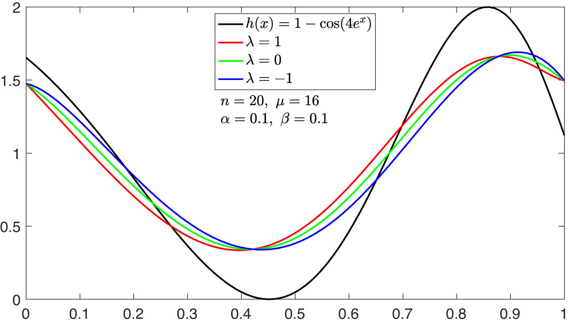
Example 1

The convergence of the ℒ n , α , β λ , μ ( h ; x ) operators to the function h ( x ) = 1 − cos ( 4 e x ) is given in Figure 1 for λ = − 1 , μ = 5 , α = 0.2 , and β = 1 and n = 10 , n = 20 , and n = 50 . The convergence improves for increasing values of n .

$Figure 1 Approximation of the operators ℒ n , α , β λ , μ ( h ; x ) {{\mathcal{ {\mathcal L} }}}_{n,\alpha ,\beta }^{\lambda ,\mu }(h;\hspace{0.33em}x) to h ( x ) = 1 − cos ( 4 e x ) h\left(x)=1-\cos (4{e}^{x}) for n = 10 n=10 , n = 20 n=20 and n = 50 n=50 , and λ = − 1 \lambda =-1 , μ = 5 \mu =5 , α = 0.2 \alpha =0.2 , and β = 1 \beta =1 .$

Figure 1

Approximation of the operators ℒ n , α , β λ , μ ( h ; x ) to h ( x ) = 1 − cos ( 4 e x ) for n = 10 , n = 20 and n = 50 , and λ = − 1 , μ = 5 , α = 0.2 , and β = 1 .

Example 2

The convergence of the ℒ n , α , β λ , μ ( h ; x ) operators to h ( x ) = 1 − cos ( 4 e x ) is given in Figure 2 for n = 20 , μ = 16 , α = 0.1 , and β = 0.1 . Here λ = 1 , λ = 0 , and λ = − 1 . It can be seen how the change in λ affects the approximation in some subintervals of [ 0 , 1 ] .

$Figure 2 Approximation of the operators ℒ n , α , β λ , μ ( h ; x ) {{\mathcal{ {\mathcal L} }}}_{n,\alpha ,\beta }^{\lambda ,\mu }(h;\hspace{0.33em}x) to h ( x ) = 1 − cos ( 4 e x ) h\left(x)=1-\cos (4{e}^{x}) for λ = 1 \lambda =1 , λ = 0 \lambda =0 , and λ = − 1 \lambda =-1 and n = 20 n=20 , μ = 16 \mu =16 , α = 0.1 , \alpha =0.1, and β = 0.1 \beta =0.1 .$

Figure 2

Approximation of the operators ℒ n , α , β λ , μ ( h ; x ) to h ( x ) = 1 − cos ( 4 e x ) for λ = 1 , λ = 0 , and λ = − 1 and n = 20 , μ = 16 , α = 0.1 , and β = 0.1 .

Example 3

The convergence of the ℒ n , α , β λ , μ ( h ; x ) operators to h ( x ) = 1 − cos ( 4 e x ) is given in Figure 3 for n = 20 , λ = 1 , α = 0.1 , and β = 0.1 . Here μ = 1 , μ = 8 , and μ = 16 . It can be seen how the change in μ affects the approximation in some subintervals of [ 0 , 1 ] .

$Figure 3 Approximation of the operators ℒ n , α , β λ , μ ( h ; x ) {{\mathcal{ {\mathcal L} }}}_{n,\alpha ,\beta }^{\lambda ,\mu }(h;\hspace{0.33em}x) to h ( x ) = 1 − cos ( 4 e x ) h\left(x)=1-\cos (4{e}^{x}) for μ = 1 \mu =1 , μ = 8 \mu =8 , and μ = 16 \mu =16 and n = 20 n=20 , λ = 1 \lambda =1 , α = 0.1 \alpha =0.1 , and β = 0.1 \beta =0.1 .$

Figure 3

Approximation of the operators ℒ n , α , β λ , μ ( h ; x ) to h ( x ) = 1 − cos ( 4 e x ) for μ = 1 , μ = 8 , and μ = 16 and n = 20 , λ = 1 , α = 0.1 , and β = 0.1 .

Example 4

Approximation error curves of three different operators ℒ n , α , β λ , μ ( h ; x ) , ℒ n , α , β λ ( h ; x ) , and ℒ n , α , β ( h ; x ) to h ( x ) = 1 − cos ( 4 e x ) is given in Figure 4 for n = 10 , α = 0.2 , β = 1 , λ = 1 , and μ = 8 . It is seen that for some x values, ℒ n , α , β λ , μ ( h ; x ) operators have a better approximation.

$Figure 4 Approximation of the operators ℒ n , α , β λ , μ ( h ; x ) {{\mathcal{ {\mathcal L} }}}_{n,\alpha ,\beta }^{\lambda ,\mu }(h;\hspace{0.33em}x) , ℒ n , α , β λ ( h ; x ) {{\mathcal{ {\mathcal L} }}}_{n,\alpha ,\beta }^{\lambda }(h;\hspace{0.33em}x) , and ℒ n , α , β ( h ; x ) {{\mathcal{ {\mathcal L} }}}_{n,\alpha ,\beta }(h;\hspace{0.33em}x) to the function h ( x ) = 1 − cos ( 4 e x ) h\left(x)=1-\cos (4{e}^{x}) for n = 10 n=10 , α = 0.2 \alpha =0.2 , β = 1 \beta =1 , λ = 1 \lambda =1 , and μ = 8 \mu =8 .$

Figure 4

Approximation of the operators ℒ n , α , β λ , μ ( h ; x ) , ℒ n , α , β λ ( h ; x ) , and ℒ n , α , β ( h ; x ) to the function h ( x ) = 1 − cos ( 4 e x ) for n = 10 , α = 0.2 , β = 1 , λ = 1 , and μ = 8 .

Example 5

Approximation error curves of three different operators ℒ n , α , β λ , μ ( h ; x ) , ℒ n , α , β λ ( h ; x ) , and ℒ n , α , β ( h ; x ) to h ( x ) = ( x − 0.5 ) sin ( π x ) are given in Figure 5 for n = 10 , α = 0.2 , β = 1 , λ = 1 , and μ = 8 . It is seen that for some x values, ℒ n , α , β λ , μ ( h ; x ) operators have a better approximation.

$Figure 5 Approximation of the operators ℒ n , α , β λ , μ ( h ; x ) {{\mathcal{ {\mathcal L} }}}_{n,\alpha ,\beta }^{\lambda ,\mu }(h;\hspace{0.33em}x) , ℒ n , α , β λ ( h ; x ) {{\mathcal{ {\mathcal L} }}}_{n,\alpha ,\beta }^{\lambda }(h;\hspace{0.33em}x) , and ℒ n , α , β ( h ; x ) {{\mathcal{ {\mathcal L} }}}_{n,\alpha ,\beta }(h;\hspace{0.33em}x) to the function h ( x ) = ( x − 0.5 ) s i n ( π x ) h\left(x)=(x-0.5)sin(\pi x) for n = 10 n=10 , α = 0.2 \alpha =0.2 , β = 1 \beta =1 , λ = 1 \lambda =1 , and μ = 8 \mu =8 .$

Figure 5

Approximation of the operators ℒ n , α , β λ , μ ( h ; x ) , ℒ n , α , β λ ( h ; x ) , and ℒ n , α , β ( h ; x ) to the function h ( x ) = ( x − 0.5 ) s i n ( π x ) for n = 10 , α = 0.2 , β = 1 , λ = 1 , and μ = 8 .

Example 6

Let h ( ξ ) = 1 − cos ( 4 e ξ ) . Error tables of the effects of changes in λ , μ , and ψ on the error rate of ℒ ψ , α , β λ , μ operators are shown in Tables 1, 3, and 4; the error rate of ℒ ψ , α , β λ operators is shown in Table 2.

From Table 1, we see that the error estimate decreases for increasing values of λ and ψ for the ℒ ψ , α , β λ , μ operators.

From Table 2, we see that the error estimate decreases for increasing values of ψ and decreasing values of λ . Furthermore, for increasing values of λ , the error degree of ℒ ψ , α , β λ , μ operators is better than the error degree of ℒ ψ , α , β λ operators, as can be seen by comparing Tables 1 and 2.

From Table 3, we see that the error estimate decreases for decreasing values of μ and increasing values of ψ for ℒ ψ , α , β λ , μ operators.

From Table 4, we see that the error estimation for the operators ℒ ψ , α , β λ , μ improves when the values of the μ parameter are held constant and those of the λ parameter are increased.

Table 1

Error estimation of ∣ ℒ ψ , α , β λ , μ ( h ; ξ ) − h ( ξ ) ∣ for μ = 8 , α = 0.1 , β = 0.1 and for different values of ψ and λ

∣ ℒ ψ , α , β λ , μ ( h ; ξ ) − h ( ξ ) ∣
	ψ = 20	ψ = 50	ψ = 100	ψ = 150	ψ = 200
λ = − 1	0.4116736961	0.210008119	0.1160155398	0.08016855484	0.06124902593
λ = − 0.5	0.4010977527	0.2077104664	0.115269711	0.07982265431	0.06105022084
λ = 0	0.3905218092	0.2055142121	0.1145238823	0.07947675379	0.06085141574
λ = 0.5	0.3813966027	0.2033179579	0.1138836775	0.07913085326	0.06065261065
λ = 1	0.383538422	0.2011217036	0.1132698351	0.07878495274	0.06045380556

Table 2

Error estimation of ∣ ℒ ψ , α , β λ ( h ; ξ ) − h ( ξ ) ∣ for α = 0.1 , β = 0.1 and for different values of ψ and λ

∣ ℒ ψ , α , β λ ( h ; ξ ) − h ( ξ ) ∣
	ψ = 20	ψ = 50	ψ = 100	ψ = 150	ψ = 200
λ = − 1	0.3959896167	0.2068348246	0.115004127	0.07970437587	0.06098370424
λ = − 0.5	0.3970831782	0.2070989471	0.1151001759	0.07974990029	0.06101016194
λ = 0	0.3981767397	0.2073630696	0.1151962249	0.07979542471	0.06103661964
λ = 0.5	0.3992703012	0.2076271921	0.1152922738	0.07984094913	0.06106307734
λ = 1	0.4003638627	0.2078913146	0.1153883227	0.07988647355	0.06108953504

Table 3

Error estimation of ∣ ℒ ψ , α , β λ , μ ( h ; ξ ) − h ( ξ ) ∣ for λ = − 1 , α = 0.1 , β = 0.1 and for different values of ψ and μ

∣ ℒ ψ , α , β λ , μ ( h ; ξ ) − h ( ξ ) ∣
	ψ = 20	ψ = 50	ψ = 100	ψ = 150	ψ = 200
μ = 1	0.402877159	0.2083391826	0.1155277043	0.07994915828	0.06112497746
μ = 5	0.4079037516	0.2092349186	0.1158064674	0.08007452774	0.0611958623
μ = 10	0.4141869924	0.210541627	0.1161549214	0.08023123957	0.06128446835
μ = 15	0.4204702332	0.2118753968	0.1165033753	0.0803879514	0.0613730744
μ = 20	0.4270425711	0.2132091667	0.1168518292	0.08054466322	0.06146168045

Table 4

Error estimation of ∣ ℒ ψ , α , β λ , μ ( h ; ξ ) − h ( ξ ) ∣ for ψ = 100 , α = 0.1 , β = 0.1 and for different values of λ and μ

∣ ℒ ψ , α , β λ , μ ( h ; ξ ) − h ( ξ ) ∣
	λ = − 1	λ = − 0.5	λ = 0	λ = 0.5	λ = 1
μ = 1	0.1155277043	0.1153619646	0.1151962249	0.1150304851	0.1148647454
μ = 5	0.1158064674	0.1153092483	0.1148120291	0.1143283093	0.113919081
μ = 10	0.1161549214	0.1152433529	0.1143375081	0.1135872563	0.1128370044
μ = 15	0.1165033753	0.1151774575	0.1139374786	0.1128462032	0.1117549279
μ = 20	0.1168518292	0.1151115621	0.1135374492	0.1121051502	0.1106728513

Acknowledgments

This work is supported by Fujian Provincial Natural Science Foundation of China (Grant No. 2024J01792).

Funding information: This work is supported by Fujian Provincial Natural Science Foundation of China (Grant No. 2024J01792).
Author contributions: All authors contributed to the study conception and design. All authors have read and approved the final version of the manuscript for publication.
Conflict of interest: The authors report having no conflicts of interest.

References

[1] S. N. Bernstein, Démonstration du théorème de Weierstrass fondée sur le calcul des probabilités, Comm. Kharkov Math. Soc. 13 (1912), 1–2. Search in Google Scholar

[2] J. L. Durrmeyer, Une formule dainversion de la transformée de Laplace: Application à la théorie des moments, Thése de 3e cycle, Faculté des Sciences de l'Université de Paris, 1967. Search in Google Scholar

[3] D. D. Stancu, Asupra unei generalizari a polinoamelor lui Bernstein, Stud. Univ. Babeş-Bolyai Ser. Math.-Phys. 14 (1969), 31–45. Search in Google Scholar

[4] Z. Ye, X. Long, and X. M. Zeng, Adjustment algorithms for Bezier curve and surface, in: International Conference on Computer Science and Education, 2010, pp. 1712–1716, DOI: http://dx.doi.org/10.1109/ICCSE.2010.5593563. 10.1109/ICCSE.2010.5593563Search in Google Scholar

[5] Q. B. Cai, B. Y. Lian, and G. Zhou, Approximation properties of λ -Bernstein operators, J. Inequal. Appl. 2018 (2018), no. 1, 61, DOI: https://doi.org/10.1186/s13660-018-1653-7. 10.1186/s13660-018-1653-7Search in Google Scholar PubMed PubMed Central

[6] Q. B. Cai and R. Aslan, On a new construction of generalized q-Bernstein polynomials based on shape parameter λ, Symmetry 13 (2021), 1919, DOI: https://doi.org/10.3390/sym13101919. 10.3390/sym13101919Search in Google Scholar

[7] K. J. Ansari and F. Usta, A generalization of Szász-Mirakyan operators based on α non-negative parameter, Symmetry 14 (2022), 1596, DOI: https://doi.org/10.3390/sym14081596. 10.3390/sym14081596Search in Google Scholar

[8] S. A. Mohiuddine and F. Özger, Approximation of functions by Stancu variant of Bernstein-Kantorovich operators based on shape parameter α, Rev. R. Acad. Cienc. Exactas Fís. Nat. Ser. A Mat. RACSAM 114 (2020), 70, DOI: https://doi.org/10.1007/s13398-020-00802-w. 10.1007/s13398-020-00802-wSearch in Google Scholar

[9] F. Özger, Weighted statistical approximation properties of univariate and bivariate λ-Kantorovich operators, Filomat 33 (2019), 3473–3486, DOI: https://doi.org/10.2298/FIL1911473O. 10.2298/FIL1911473OSearch in Google Scholar

[10] R. Aslan and M. Mursaleen, Some approximation results on a class of new type λ-Bernstein polynomials, J. Math. Inequal. 16 (2022), 445–462, DOI: https://doi.org/10.7153/jmi-2022-16-32. 10.7153/jmi-2022-16-32Search in Google Scholar

[11] Q. B. Cai, The Bézier variant of Kantorovich type λ-Bernstein operators, J. Inequal. Appl. 2018 (2018), 90, DOI: https://doi.org/10.1186/s13660-018-1688-9. 10.1186/s13660-018-1688-9Search in Google Scholar PubMed PubMed Central

[12] V. A. Radu, P. N. Agrawal, and J. K. Singh, Better numerical approximation by λ-Durrmeyer-Bernstein type operators, Filomat 35 (2021), 1405–1419, DOI: https://doi.org/10.2298/FIL2104405R. 10.2298/FIL2104405RSearch in Google Scholar

[13] G. Zhou and Q. B. Cai, Approximation properties of generalized λ-Bernstein operators, Open Math. (In Review). Search in Google Scholar

[14] Q. B. Cai, R. Aslan, F. Özger, and H. M. Srivastava, Approximation by a new Stancu variant of generalized (λ,μ)- Bernstein operators, Alex. Eng. J. 107 (2024), 205–214, DOI: https://doi.org/10.1016/j.aej.2024.07.015. 10.1016/j.aej.2024.07.015Search in Google Scholar

[15] Q. B. Cai and Z. Guorong, Approximation properties of (λ,μ)-Bernstein-Durrmeyer operators, Math. Methods Appl. Sci. 48 (2024), no. 5, 5946–5953, DOI: https://doi.org/10.1002/mma.10647. 10.1002/mma.10647Search in Google Scholar

[16] F. Altomare and M. Campiti, Korovkin-Type Approximation Theory and its Applications, De Gruyter Studies in Mathematics 17, Walter de Gruyter, Berlin-New York, 1994. 10.1515/9783110884586Search in Google Scholar

[17] F. Altomare, Korovkin-type theorems and approximation by positive linear operators, Surv. Approx. Theory 5 (2010), 92–164. Search in Google Scholar

[18] E. Quak, Lp-error estimates for positive linear operators using the second-order τ-modulus, Anal. Math. 14 (1988), 259–272. 10.1007/BF01906850Search in Google Scholar

[19] M. W. Müller, Approximation by Cheney-Sharma-Kantorovich polynomials in the Lp-metric, Rocky Mountain J. Math. 19 (1989), no. 1, 281–291. 10.1216/RMJ-1989-19-1-281Search in Google Scholar

[20] H. Johnen, Inequalities connected with the moduli of smoothness, Mat. Vesnik 9 (1972), no. 24, 289–303. Search in Google Scholar

[21] A. Zygmund, Trigonometric Series I, II, Cambridge University Press, New York, 1959. Search in Google Scholar

Received: 2024-11-08

Revised: 2025-03-29

Accepted: 2025-04-28

Published Online: 2025-07-31

This work is licensed under the Creative Commons Attribution 4.0 International License.

Articles in the same Issue

https://doi.org/10.1515/dema-2025-0132

Keywords for this article

λ-Bernstein operators; Durrmeyer operators; Stancu operators; modulus of continuity; Bézier basis functions; L p approximation

Creative Commons

BY 4.0