
Admissibility conditions for Riemann data in shallow water theory
-
Martin O. Paulsen


Abstract
Consideration is given to the shallow-water equations, a hyperbolic system modeling the propagation of long waves at the surface of an incompressible inviscible fluid of constant depth. It is well known that the solution of the Riemann problem associated to this system may feature dry states for some configurations of the Riemann data. This article will discuss various scenarios in which the Riemann problem for the shallow water system arises in a physically reasonable sense. In particular, it will be shown that if certain physical assumptions on the disposition of the Riemann data are made, then dry states can be avoided in the solution of the Riemann problem.
1 Introduction
Many physical systems can be described by systems of conservation laws. Such systems are first-order quasilinear partial differential equations, and for one-dimensional problems they can be written in the general form
where
Due to the special nonlinear structure of such systems, solutions naturally develop discontinuities in time, even if the original state of the system is given by a smooth function of x. Once a discontinuity has developed, solutions of the system need to be interpreted in a weak sense. If the solution is to include a jump between a left state
The Riemann problem distills the essence of the problem of singularity formation into a simple initial-value problem where the initial data have a prescribed discontinuity. For the system above, the Riemann problem would prescribe initial data of the form
where
In the present work, our focus is on the well-known shallow-water system which appears in the general form (1) when defining the principal unknown vector
In physical terms, the unknown
The solution of the Riemann problem for the shallow-water equations is well known, and can be found in many texts on conservation laws (cf. [2], [12]). One way to normalize the problem is to consider the left state
As can be gleaned from Figure 1, the condition that h be non-negative restricts the analysis to the right half-plane in the
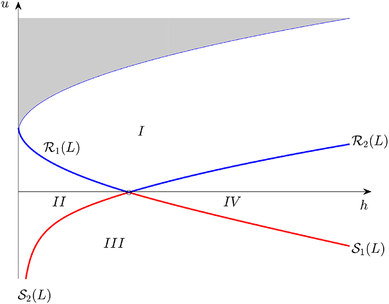
Phase space for a particular left state
Recall that the shallow-water assumption applies to surface waves that are slowly varying, and a shock represents a bore (i. e., a traveling hydraulic jump) where the shock structure which may feature oscillations or turbulent structures) has been neglected [7], [22], [28]. If this physical interpretation is taken as a point of departure, then it appears that a Riemann problem may develop from the collision of two bores, and a natural admissibility condition would be to consider only such Riemann problems. Thus we will study the history of the Riemann problem, or more succinctly the backwards problem for
Note that a Riemann problem could also develop from certain initial data which are arranged in such a way that the solution lines up at some time so as to give a perfect Riemann problem. While this is possible, it would clearly be unstable to even the smallest perturbations. On the other hand, one might also consider the collision of three or more traveling hydraulic jumps, or the collision between rarefaction waves and shocks, but these situations are so unlikely to happen that they would constitute a set of measure zero in the configuration space. In the current work, we focus on the origin of the Riemann problem which can be represented by a set of non-zero measure in the configuration space given by the phase plane.
The outline of this paper is as follows. In sections 2 and 3, a short discussion of the properties of basic admissible waves for the shallow-water system is given, and the standard solution of the Riemann problem is explained in section 4. This is standard fare, but we need various formulas in order to set up the problem to be attacked. In sections 5, 6, and 7, Riemann problems originating from various configurations are investigated. Some ramifications of our results are discussed in the Conclusion.
2 Shock waves and bore properties
As already mentioned above, the shallow-water system can be written in terms of mass and momentum conservation in the form
A derivation of this system from first principles can be found in [25], where it is also shown that the conservation of energy is formulated as
Discontinuous solutions develop naturally in this system even in the case of flat bathymetry which is under study here. In the case when the solution features jumps, the imposition of mass and momentum conservation leads to an energy loss (see [23]) which has been the subject of a number of studies [3], [4], [5], [6], [15], [26]. In the context of the conservation laws, the energy loss means that (6) becomes an inequality, which is then taken as the mathematical entropy in order to pick out physically reasonable discontinuous solutions.
In the context of the shallow-water equations (4) and (5) the Rankine-Hugoniot condition (2) yields the following relations:
Combining these two equations enables us to find an expression for
A useful observation to be used later is that the fluid velocity of u on
where the minus sign refers to the
The Hugoniot loci may also be described in terms of the momentum
Taking the second derivative of these expressions shows that these curves are strictly concave and convex, respectively:
Finally, the speed of the discontinuity may be found from the Rankine-Hugoniot condition as
Next, let us discuss the entropy condition for shock waves. It is well known [12], [24] that it is necessary to impose both the Rankine-Hugoniot and the entropy condition to ensure uniqueness of a solution. In the context of the shallow-water theory, the mechanical energy serves as a mathematical entropy. In fact, it is well known that energy is lost in a shock either due to turbulence or the continuous creation of surface oscillations [3], [6], [11], [13], [14], [25]. Similar considerations can be used in various other applications, such as for example in the context of porous media [1].
In the present case, the expected loss of mechanical energy is enforced by imposing the inequality
for discontinuous solutions. It is also convenient to introduce the relative mass flux m by
Using m, we can express the rate at which energy is lost at the shock by
Note that since we always require
Properties of shock curves
| Hugoniot locus | Fluid velocity
|
Momentum
|
|
|---|---|---|---|
|
|
|
|
|
|
|
|
|
Jump properties on
| Hugoniot locus |
|
|
|---|---|---|
| Increase/decrease in flow depth |
|
|
| Front speed |
|
|
| Relative mass flux |
|
|
| Velocity relation |
|
|
| Velocity relation |
|
|
| Velocity relation |
|
|
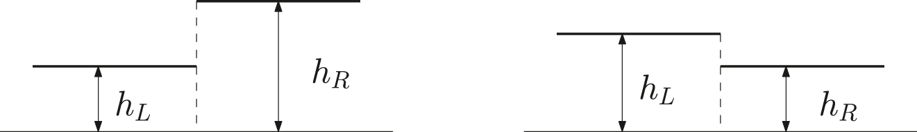
Left panel: bore with flow depth
One should also remark that both
where
A geometrical representation of the Lax entropy condition in the
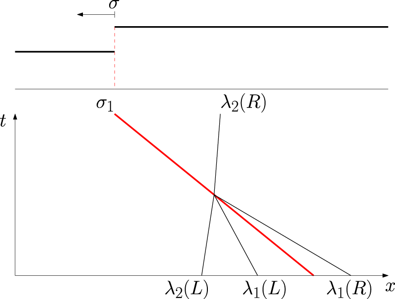
Left moving bore with speed
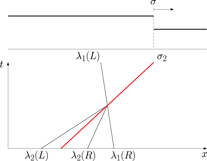
Right moving bore with speed
3 Rarefaction waves
Following the classical theory (presented for example in [10], [28], [12]) we seek traveling wave solutions of the form
The solution is then given by the integral of (16). We may now exploit this insight using the theory of Riemann invariants
Along a Riemann invariant, the solution must therefore satisfy
Hence, for a given left state we may write the rarefaction wave solution as follows
By comparison, one can also show that
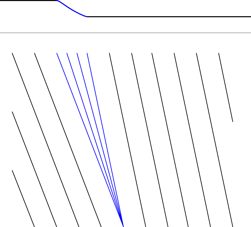
Left moving rarefaction wave smoothly varying between
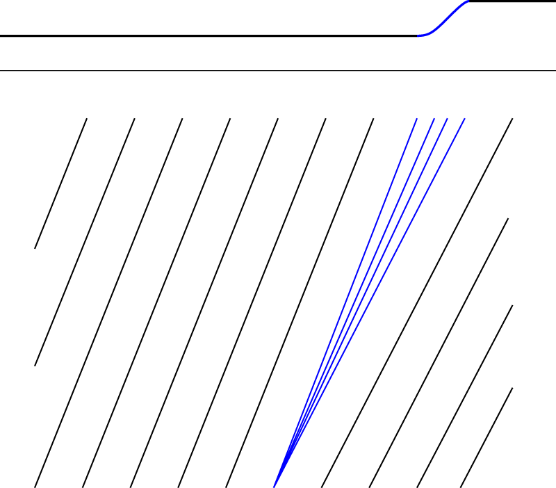
Right moving rarefaction wave providing a smooth transition between
In fluid mechanics, some authors refer to these waves as negative surges resulting from a decrease in flow depth [9]. Interestingly, Peregrine was able to show that a negative surge together with a bore advancing in positive direction originates from the collision of two fast shocks [21]. Therefore, we will discuss the development of the Riemann problem from a collision of two
4 General solution of the Riemann problem
Using the results from sections 3 and 4, the general solution of the Riemann problem can be fond using the rarefaction curves defined by (19) and (20)
and the shock curves (7) and (8)
In the following, it will be convenient to plot the integral curves and shock curves for a particular left state
which is simply the secant line joining the two states. For example, any right state given on the
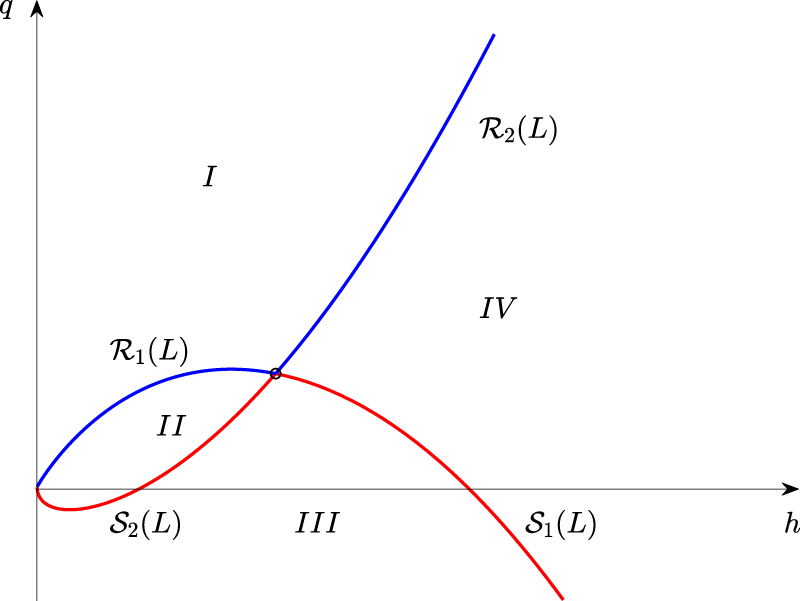
Phase-space in
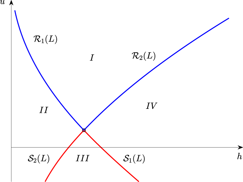
Phase-space in
Solution in region
Solution in region
5 Development of the Riemann problem from a collision of
S
2
and
S
1
shocks
In this section, we will discuss the origin of the Riemann problem from a collision of two bores. It is most convenient to focus the discussion by assuming that a left state is given. With this proviso, we will prove that the Riemann problem associated to certain right states in region
Backwards problem in
In order to understand how a given Riemann problem develops, we consider the backwards problem for
As indicated in Figure 12, the solution of the Riemann problem for a right state in region
Forward problem in
The Riemann problem at
Theorem 1
Suppose that a left state
Proof. Step 1
Existence of a center state: We need to prove there is a center state connecting two colliding shock waves satisfying the bore conditions. Guided by the discussion above, and using an argument similar to one used in [16], we seek a point
As already indicated in Table 1, taking the derivative
Keeping the right state fixed, and varying
Step 2
Head-on collision and overtaking bores: We now analyze whether the center state found in Step 1 actually leads to a collision of shocks. As will be shown presently, the center state will always give rise to a Riemann problem originating from either a head-on collision or an overtaking collision of two shocks. In order to prove this statement, we first note that having
when substituting
In addition, differentiating
Hence we conclude that
Step 3
Inadmissible connections: Regarding the last statement of the theorem, we will now argue that for a right state in region I,
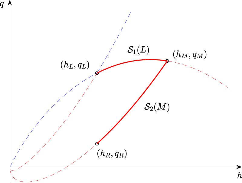
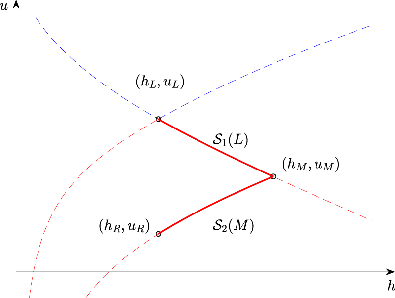
Before proceeding, we will offer some clarifying remarks. For the shallow-water equation, given a left state we can always connect any right state with a middle state as mentioned earlier. Once you know the right state it is then possible go back through a center state. We find it instructive to describe the solution for two particular states in both phase-space and in

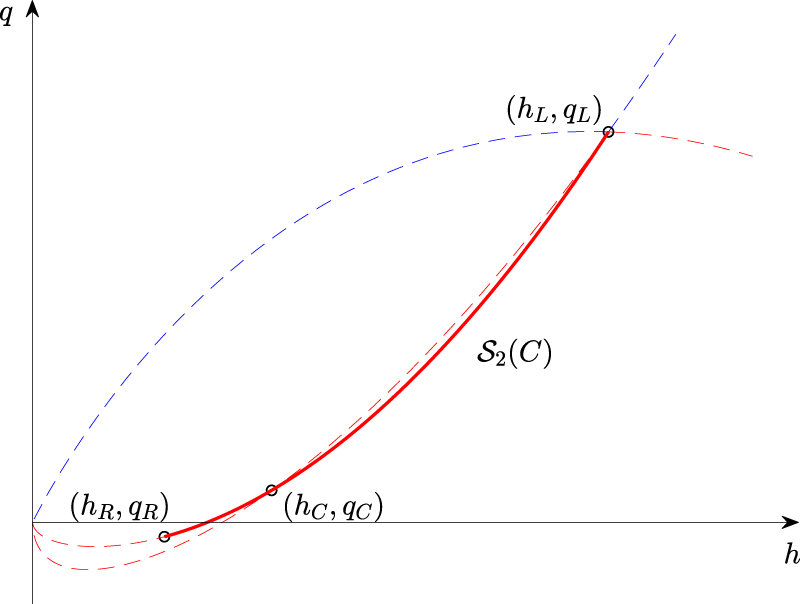
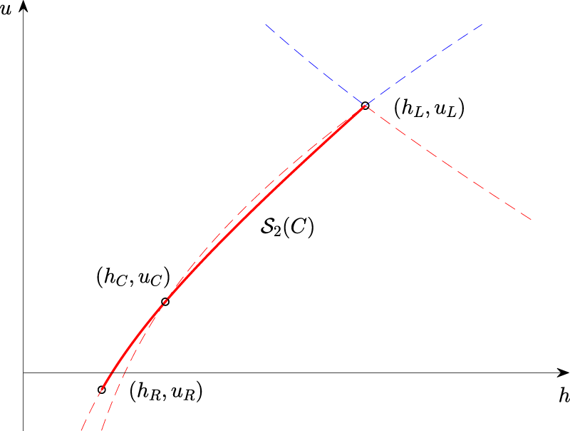
Development of the Riemann problem in phase space.
Development of the Riemann problem in
6 Development of the Riemann problem from a collision of two
S
2
shocks
Consideration will now be given to the Riemann problem arising from a
On the other hand, if the center state is to be connected to the right state by an
Putting these two formulas together defines the region of all possible right states as
We have the following theorem.
Theorem 2
Suppose that a left state
On the other hand, it is not possible for a Riemann problem to develop from a
Proof
First of all, the definition of the set
To see that the state
It needs to be shown that
Evaluating the first and second derivative of
and
By inspection, we see that
Lemma 1
Given
Proof
Evaluating the derivative
Next multiply with the positive number
Letting
Evidently, the proof will be achieved if it can be shown that the function
is positive for all
Note that
Finally, denote the shock speeds of the backwards problem by
and
Now recall that it was proved in Section 3 that the function
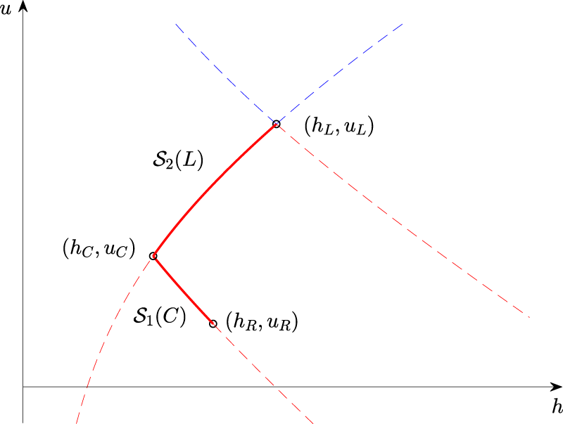
A particular example of the backwards problem is represented in phase space for
In Figure 17, we observe that
Backwards problem in
Backwards problem in
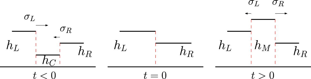
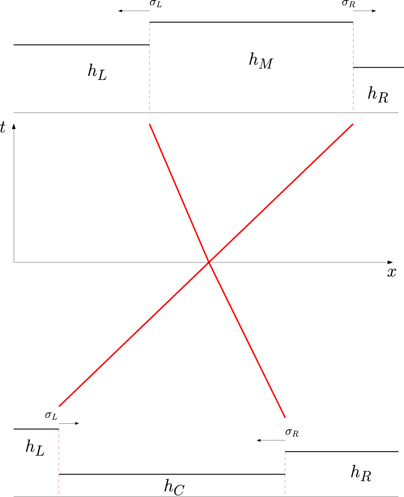
Two colliding bores forming the Riemann Problem.
7 Development of the Riemann problem from a collision of two
S
1
shocks
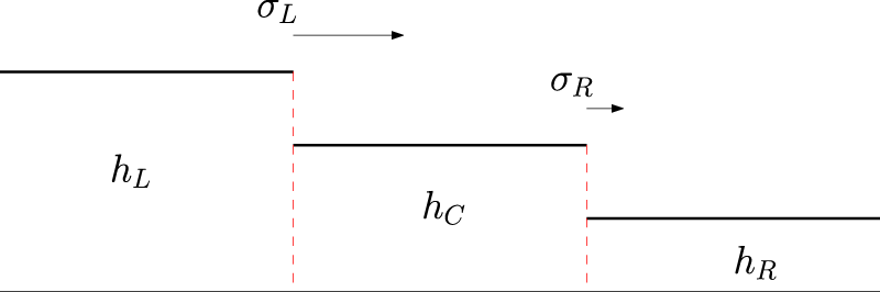
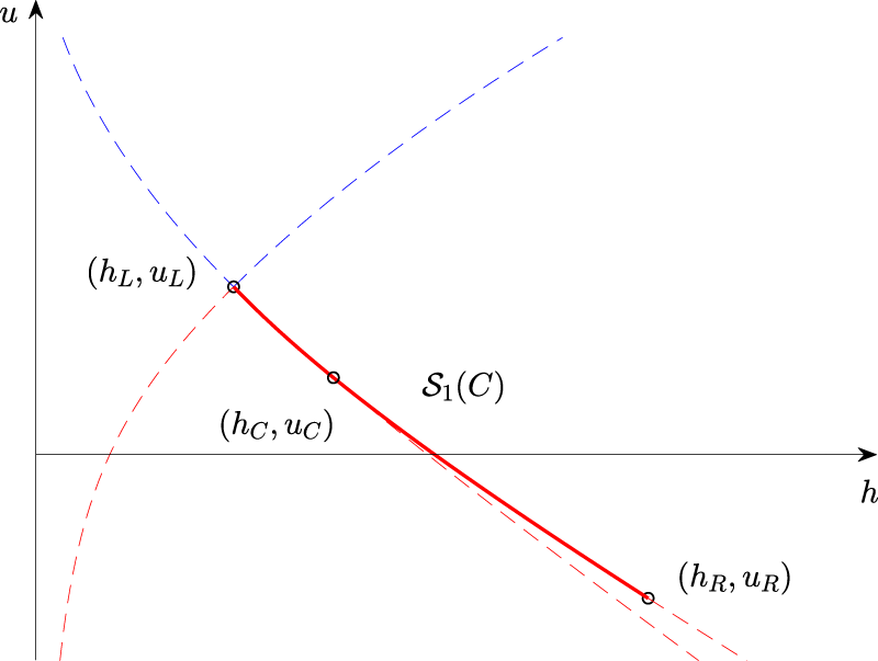
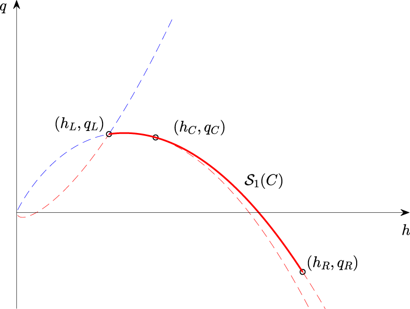
The final case to be considered is when a Riemann problem develops from the collision between two
As before, we consider the left state given. It is then straightforward to see that the center state in the backwards problem must lie in the Rankine-Hugoniot locus
On the other hand, if the center state is to be connected to the right state by an
Putting these two formulas together defines the region of all possible right states as
We have the following theorem.
Theorem 3
Suppose that a left state
On the other hand, it is not possible for a Riemann problem to develop from a
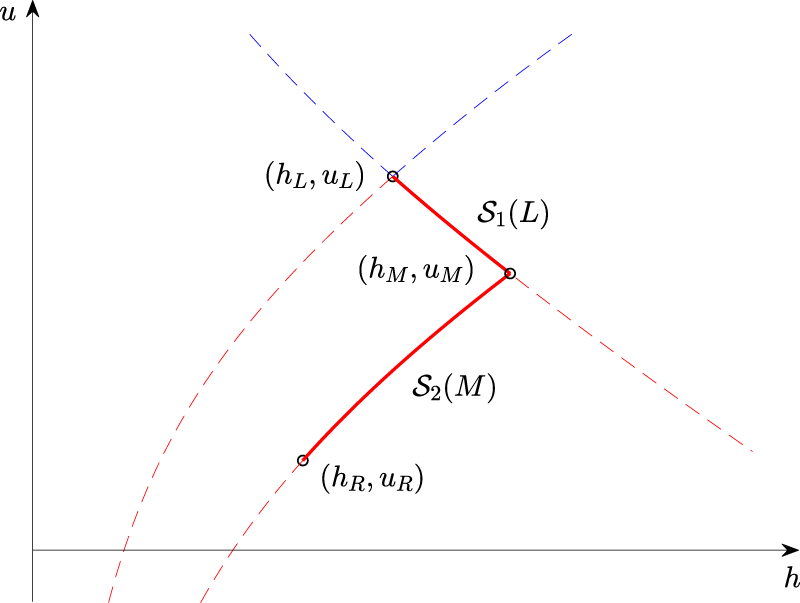
The proof of theorem 3 is virtually the same as that of Theorem 2, except for changing signs in the right places. From Figure 19, we observe that both bores are moving to the left due to a negative slope. However, the right state moves faster than the left. This is also true in general since
Backwards problem in
Backwards problem in
8 Conclusion
In this article, we have considered the Riemann problem associated to the shallow-water equations. The study of the Riemann problem is important when trying to understand the behavior of solutions of a system of conservation laws. For example the Riemann problem can used as a tool in the front-tracking method where general initial data are decomposed into piecewise constant functions which gives rise to a series of Riemann problems [12]. This approach is used in existence proofs and numerical schemes, but one may face difficulties interpreting solutions of the Riemann problem for the shallow-water equations in the case when the solution includes a dry region (
In the present work, we have imposed the condition that the Riemann problem should arise from the collision of two bores. With this condition in place, we were able to show that solutions of the Riemann problem do not feature cavitation. In summary, for a given left state, the collision of an
Funding source: Norges Forskningsråd
References
[1] I. Aavatsmark, “Kapillarenergie als Entropiefunktion,” Z. Angew. Math. Mech., vol. 69, pp. 319–327, 1989, https://doi.org/10.1002/zamm.19890691002.Suche in Google Scholar
[2] I. Aavatsmark, Bevarelsesmetoder for hyperbolske differensialligninger, Lecture Notes, University of Bergen, 2003, p. 140.Suche in Google Scholar
[3] A. Ali and H. Kalisch, “Energy balance for undular bores,” Compt. Rend. Mecanique, vol. 338, pp. 67–70, 2010, https://doi.org/10.1016/j.crme.2010.02.003.Suche in Google Scholar
[4] A. Ali and H. Kalisch, “Mechanical balance laws for Boussinesq models of surface water waves,” J. Nonlinear Sci., vol. 22, pp. 371–398, 2012, https://doi.org/10.1007/s00332-011-9121-2.Suche in Google Scholar
[5] A. Ali and H. Kalisch, “A dispersive model for undular bores,” Anal. Math. Phys., vol. 2, pp. 347–366, 2012, https://doi.org/10.1007/s13324-012-0040-7.Suche in Google Scholar
[6] T. Benjamin and J. Lighthill, “On cnoidal waves and bores,” Proc. R. Soc. A, vol. 224, pp. 448–460, 1954, https://doi.org/10.1098/rspa.1954.0172.Suche in Google Scholar
[7] M. Bjørkavåg and H. Kalisch, “Wave breaking in Boussinesq models for undular bores,” Phys. Lett. A, vol. 375, pp. 1570–1578, 2011, https://doi.org/10.1016/j.physleta.2011.02.060.Suche in Google Scholar
[8] S. Bianchini and A. Bressan, “Vanishing viscosity solutions of nonlinear hyperbolic systems,” Ann. of Math., vol. 161, pp. 223–352, 2005, https://doi.org/10.4007/annals.2005.161.223.Suche in Google Scholar
[9] H. Chanson, Hydraulics of open channel flow, Arnold, 1999.Suche in Google Scholar
[10] L. C. Evans, Partial Differential Equations. 1st ed. Graduate Studies in Mathematics, vol. 19, Providence, RI, American Mathematical Society, 1998.Suche in Google Scholar
[11] H. Favre, Ondes de Translation, Paris, Dunod, 1935.Suche in Google Scholar
[12] H. Holden and N. H. Risebro, Front Tracking for Hyperbolic Conservation Laws, New York, Springer, 2015.10.1007/978-3-662-47507-2Suche in Google Scholar
[13] F. M. Henderson, Open Channel Flow, Prentice Hall, 1996.Suche in Google Scholar
[14] H. G. Hornung, C. Willert and S. Turner, “The flow field downstream of a hydraulic jump,” J. Fluid Mech., vol. 287, pp. 299–316, 1995, https://doi.org/10.1017/s0022112095000966.Suche in Google Scholar
[15] H. Kalisch, Z. Khorsand and D. Mitsotakis, “Mechanical balance laws for fully nonlinear and weakly dispersive water waves,” Physica D, vol. 333, pp. 243–253, 2016, https://doi.org/10.1016/j.physd.2016.03.001.Suche in Google Scholar
[16] H. Kalisch and D. Mitrović, “Singular solutions of a fully nonlinear 2x2 system of conservation laws,” Proc. Edinb. Math. Soc., vol. 55, pp. 711–729, 2012, https://doi.org/10.1017/s0013091512000065.Suche in Google Scholar
[17] P. D. Lax, “Hyperbolic systems of conservation laws II,” Comm. Pure Appl. Math., vol. 10, pp. 537–566, 1957, https://doi.org/10.1002/cpa.3160100406.Suche in Google Scholar
[18] R. J. LeVeque, Finite Volume Methods for Hyperbolic Problems, Cambridge, Cambridge University Press, 2002.10.1017/CBO9780511791253Suche in Google Scholar
[19] T. P. Liu, “Existence and uniqueness theorems for Riemann problems,” Trans. Amer. Math. Soc., vol. 212, pp. 375–382, 1975, https://doi.org/10.1090/s0002-9947-1975-0380135-2.Suche in Google Scholar
[20] T. P. Liu, “The Riemann problem for general systems of conservation laws,” J. Differ. Equ., vol. 18, pp. 218–234, 1975, https://doi.org/10.1016/0022-0396(75)90091-1.Suche in Google Scholar
[21] D. H. Peregrine, “Water-wave interaction in the surf zone,” in Coastal Engineering Proceedings 1974, 1975, pp. 500–517.10.1061/9780872621138.031Suche in Google Scholar
[22] D. H. Peregrine, “Calculations of the development of an undular bore,” J. Fluid Mech., vol. 25, p. 321, 1966, https://doi.org/10.1017/s0022112066001678.Suche in Google Scholar
[23] L. Rayleigh, “Note on Tidal Bores,” Proc. Roy. Soc. London Ser. A, vol. 81, pp. 448–449, 1908, https://doi.org/10.1098/rspa.1908.0102.Suche in Google Scholar
[24] M. Renardy and R. C. Rogers, An Introduction to Partial Differential Equations, Texts in Applied Mathematics, vol. 13, New York, Springer-Verlag, 1993.Suche in Google Scholar
[25] J. J. Stoker, Water Waves: The Mathematical Theory with Applications, New York, Interscience Publishers, 1957.Suche in Google Scholar
[26] B. Sturtevant, “Implications of experiments on the weak undular bore,” Phys. Fluids, vol. 8, pp. 1052–1055, 1965, https://doi.org/10.1063/1.1761354.Suche in Google Scholar
[27] C. Tsikkou, “Hyperbolic conservation laws with large initial data. Is the Cauchy problem well-posed?,” Quart. Appl. Math., vol. 68, pp. 765–781, 2010, https://doi.org/10.1090/s0033-569x-2010-01208-9.Suche in Google Scholar
[28] G. B. Whitham, Linear and Nonlinear Waves, New York, Wiley, 1974.Suche in Google Scholar
© 2020 Walter de Gruyter GmbH, Berlin/Boston
Artikel in diesem Heft
- Frontmatter
- General
- Remote magnetically controlled drug release from electrospun composite nanofibers: design of a smart platform for therapy of psoriasis
- Dynamical Systems & Nonlinear Phenomena
- A modified simple chaotic hyperjerk circuit: coexisting bubbles of bifurcation and mixed-mode bursting oscillations
- Dynamics of a discrete-time system with Z-type control
- Dynamic response of axially loaded end-bearing rectangular closed diaphragm walls
- Hydrodynamics
- Admissibility conditions for Riemann data in shallow water theory
- Numerical study on the rotating electro-osmotic flow of third grade fluid with slip boundary condition
- Solid State Physics & Materials Science
- Ultrasonic study of Si-oil based magneto-rheological fluid
- Electromagnetic propagation characteristics of one-dimensional photonic crystals with metal layers in quasi-parity-time (PT)-symmetric system
- Thermodynamics & Statistical Physics
- Combined influence of axial electron temperature and exponential plasma density ramp on the self-focusing of a chirped laser in plasma