
Dynamics of a discrete-time system with Z-type control
-
Shilpa Garai


Abstract
In community ecology, the stability of a predator–prey system is a considerably desired issue; as a result, population control of a predator–prey system is very important. The dynamics of continuous-time models with Z-type control is studied earlier. But, the effectiveness of the Z-type control mechanism in a discrete-time set-up is lacking. First, we consider a Lotka–Volterra type discrete-time predator–prey model. We observe that without control, the system exhibits rich dynamical behaviors including chaotic oscillations. We apply the Z-control mechanism in both direct and indirect ways to the system and observe that in both cases, controllers have the property to drive the populations of the system to the desired state. We conduct numerical simulation as supporting evidence of our analytical results.
1 Introduction
Ecology is the branch of biology, which addresses the full scale of life of species together with their physical environment that spans the entire planet [1]. The study of ecology provides information about the interactions among living and non-living things and the energy transfer from one trophic level to another trophic level through which the organisms survive in the world. Community ecology studies the interactions between the populations, for example, competition and predation [2]. These relationships may be represented through a food web. A food web consists of several food chains and a food chain shows how the organisms are related to each other by their food [3]. Each level of a food chain represents a different trophic level and food energy is transferred from one trophic level to another trophic level by which the ecological balance is maintained [4]. But recently, the ecological balance is disturbed due to the changing climate, habitat loss, degradation, etc., [5]. For these reasons, animal and plant species are moving in the way of destruction, which changes the ecosystem significantly. So, the preservation of ecological balance is very important and it will be possible if all species remain in the desired state.
To describe and analyze the predator–prey relationships, mathematical model has become a very important tool for its huge applications, where the models are usually framed by a set of relations and variables [6]. In mathematical modeling, there are mainly two alternative frameworks, discrete-time set-up, and continuous-time set-up, within which model variables develop over time. Continuous-time systems are described by differential equations. On the other hand, discrete-time systems are described by difference equations [7]. Difference equations are used to compute the population size at discrete points in time. Discrete-time models are more appropriate in small population size or when the population having no overlapping generation. Many annual plants and insect species (like ants, grasshoppers, budmoths, and cicadidae, etc.,) have no overlap in their successive generations, so their populations obey discrete-time behavior [8], [9]. On the other hand populations with overlapping generations are modeled by continuous-time model [10]. However, we can get rich and complex dynamics in just one-dimensional discrete-time model. For instance, chaos can be exhibited in one-dimensional discrete-time model [9]. Unfortunately, empirical evidence to support this theoretical possibility is scarce. Turchin and Taylor (1992) [11] fitted a minimum of 18 year’s time-series data for 14 insect and 22 vertebrate populations by using single species difference equation model. They observed chaos in only one insect population (Phyllaphis fagi). They concluded that the complete spectrum of dynamical behaviors, ranging from stability to chaos, is likely to be found among natural populations. Costantino et al. (1995) [12] reported a joint theoretical and experimental study to test the hypothesis that changes in demographic parameters may change the predictability of population fluctuations. They predicted by using single species difference equation model (three-dimensional map for larva, pupa, and adult), that changes in adult mortality rate would produce a substantial shift in population dynamic behavior. By experimentally manipulating the adult mortality rate of flour beetle Tribolium, they also observed changes in the dynamics from stable fixed points to periodic cycles and aperiodic oscillations that corresponded to the prediction of the mathematical model. On the other hand, for showing chaotic behavior in a continuous-time autonomous model minimum three species are needed [13], [14]. Discrete-time models are easy to understand, develop, and simulate. For modeling experimental data, which are almost always discrete, it is mostly suitable [15].
Various types of mathematical models have been developed to describe and analyze different types of biological phenomena by which one can predict the future state of a system. Historically, at first, a single species population model was formulated by Malthus [16]. Also, it is well known that many ecological models have been developed by incorporating logistic growth term for the prey species and Holling type-II functional response for the predator species after the pioneering work of Lotka and Volterra [17], [18], [19]. In recent years, the ecological balance is one of the most desirable and widely investigated issue in both continuous-time and discrete-time systems [8], [20]. If the population sizes of interacting species are controlled anyhow, then the ecological balance may be maintained. Different biological phenomena like imposition of a population floor [21], [22], addition of refugia [23], omnivory [24], intraspecific density dependence [25], toxic inhibition [26], spatial effect [27], dispersal [28], [29], [30], predator switching [31], [32], Allee effect [33], additional predator [34], additional food [35], harvesting of predator [36], fear effect [37], [38], etc., may increase the ecological stability. Although a system may be stable by incorporating these phenomena, these are not always capable to achieve desired population abundance. But there is an effective and powerful control strategy named Z-type control mechanism which is capable to achieve ecological balance and to drive the abundance of a species to the desired state. The Z-control mechanism can keep species away from extinction and improve ecosystem stability.
The Z-type control mechanism is a neural dynamic approach. It is an error-based method that can be used to control a system described in the form of a set of equations, which are termed as system equations. In this method, the design formula guarantees that each component of the error function converges to zero. This idea is performed by compelling the difference between the actual output and the desired output of the system to be zero. The Z-type control can be applied through both the direct and indirect ways in a system. In a direct way, control can be applied to all the variables simultaneously for controlling the dynamics of the system. In indirect control, if one variable needs to be controlled, then the control is applied to another variable.
Many researchers have investigated different types of continuous-time models with the Z-type control mechanism. Zhang et al. [39] considered the Lotka–Volterra predator–prey model with the Z-control mechanism in both direct and indirect ways to drive the prey and predator populations to the desired states for preventing species from extinction. Lacitignola et al. [40] studied a generalized predator–prey system with Z-type control. Nadim et al. [41] explored the possible applications of fear in the prey population by changing the density of the predator population and observed that after incorporating the Z-control mechanism the system reaches to a stable steady-state. Alzahrani et al. [42] studied an eco-epidemiological model with Z-type controller on the predator population and observed that the disease, as well as the chaotic oscillations, can be removed from the system. Samanta et al. [43] proposed and analyzed an epidemic model with the Z-control mechanism. Recently, Lacitignola et al. [44] applied the Z-type approach to control backward bifurcation phenomena in a SIR model. Very recently, Senapati et al. [45] studied an SI type disease model employing Z-control approach through the removal of the population.
So many continuous-time predator–prey models equipped with the Z-type controller have been developed successfully, but as far as our knowledge goes, there is no such investigation on the predator–prey model with Z-type control in the discrete-time system. This is the first liberal attempt to investigate the predator–prey model with the Z-type control mechanism in a discrete-time set-up.
Here, we consider a Lotka–Volterra type predator–prey model in discrete-time set-up and apply Z-type control mechanism in both direct and indirect ways for controlling the populations. The rest of the paper is ordered as follows. In Section 2, a direct Z-control mechanism is applied to a predator–prey model. In Section 3, an indirect Z-controller on the predator population is applied to control the prey population density. In Section 4, we come to the end of the paper with final remarks, in which we discuss how the inclusion and/or exclusion of species into or from the system depending on the sign of the update parameter helps to get a desired state of the system.
2 Direct control of populations
In this section, we discuss briefly the general design procedure of direct Z-control laws for a discrete-time system. To do this, a controller group is considered for the simultaneous control of prey and predator populations by taking the exogenous measures for both species and applying the Z-type dynamic method. We also check the convergence performance of the controller group explicitly.
2.1 Controller-group design
Here, we consider a general two-dimensional model in discrete-time set-up as follows:
After introducing two exogenous measures for interacting species, the above model takes the following form:
where the exogenous measures
At first, a vector-valued error function
Secondly, the design formula is defined in such a way that the error function approaches to zero and it is adopted as:
where
Substituting Eq. (2.3) in Eq. (2.4), we get
Now from Eq. (2.2) and (2.5), finally we obtain the analytical expression of the control variables as:
which is the Z-type controller group for the simultaneous control of species-I and species-II.
2.2 Theoretical analysis
In this subsection, the convergence performance of the Z-type controller group for the above generalized two-dimensional model is examined theoretically. Here, it is shown that each component of the tracking error vector for the above model (2.2) converges to zero.
Theorem 1:
For a bounded desired state
Proof: According to the design procedure of Z-type controller group (2.6), we have
where, the design parameter is
Now, we evaluate the Jacobian matrix (J) for the above system of equations (2.7) and it is given as follows:
The eigenvalues of the matrix J are
2.3 Example of direct control
In this subsection, we consider a Lotka–Volterra type predator–prey model in discrete-time set-up as follows:
where,
where, the exogenous measures
which is the controller group for the simultaneous control of prey and predator populations.
Therefore, using the error function and the design formula we can obtain the explicit expressions for inputs
2.4 Numerical simulation
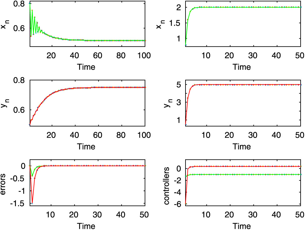
In this subsection, explanatory simulation results are given to show the feasibility of the controller group (2.10) for the simultaneous control of prey and predator populations. Here, our main goal is to show numerically, how the different dynamical behavior of the uncontrolled system (2.8) (chaotic oscillation, periodic oscillation, and stable dynamics) are controlled by the Z-type controller group (2.10) and also to show both prey and predator populations reach to the desired states in each case. Here, we consider the value of the parameters as
with initial condition
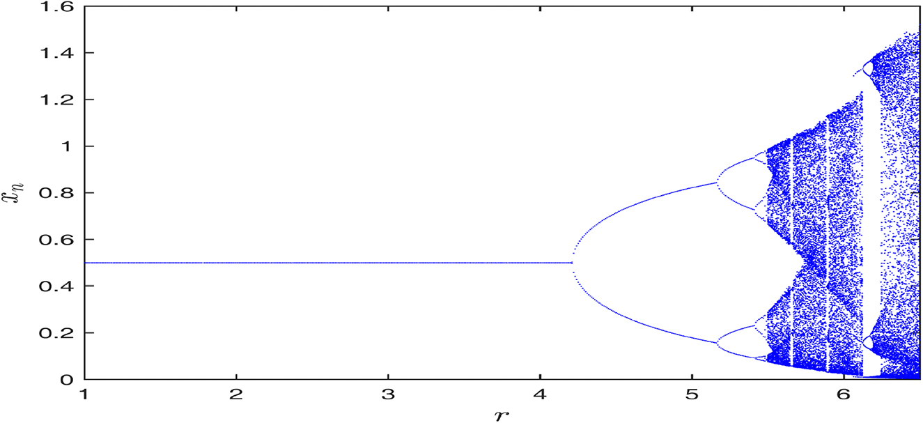
Figure shows the bifurcation diagram for the prey species of the uncontrolled system (2.8). Here bifurcating parameter is r and other parameter values are taken as
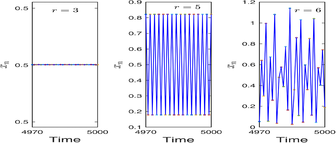
Switching of dynamics of the uncontrolled system (2.8) for different values of r. Left figure shows stable dynamics for
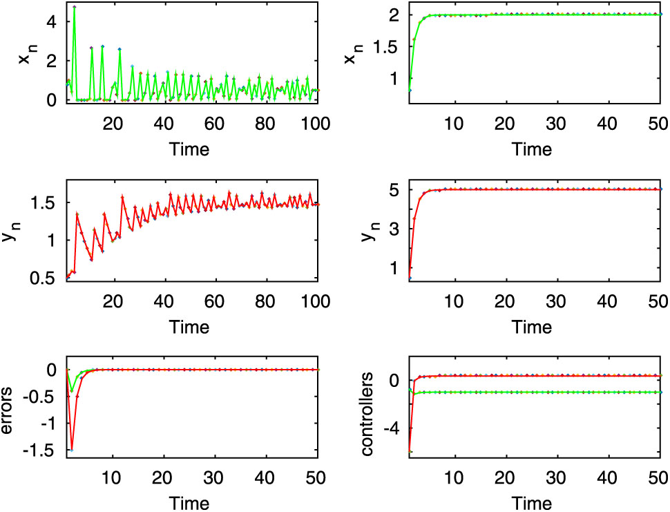
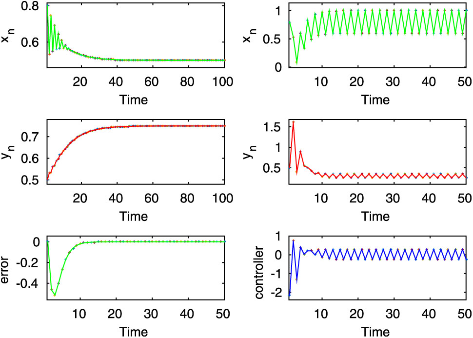
Here, the first two rows of left column show the chaotic oscillation for the uncontrolled system (2.8) when
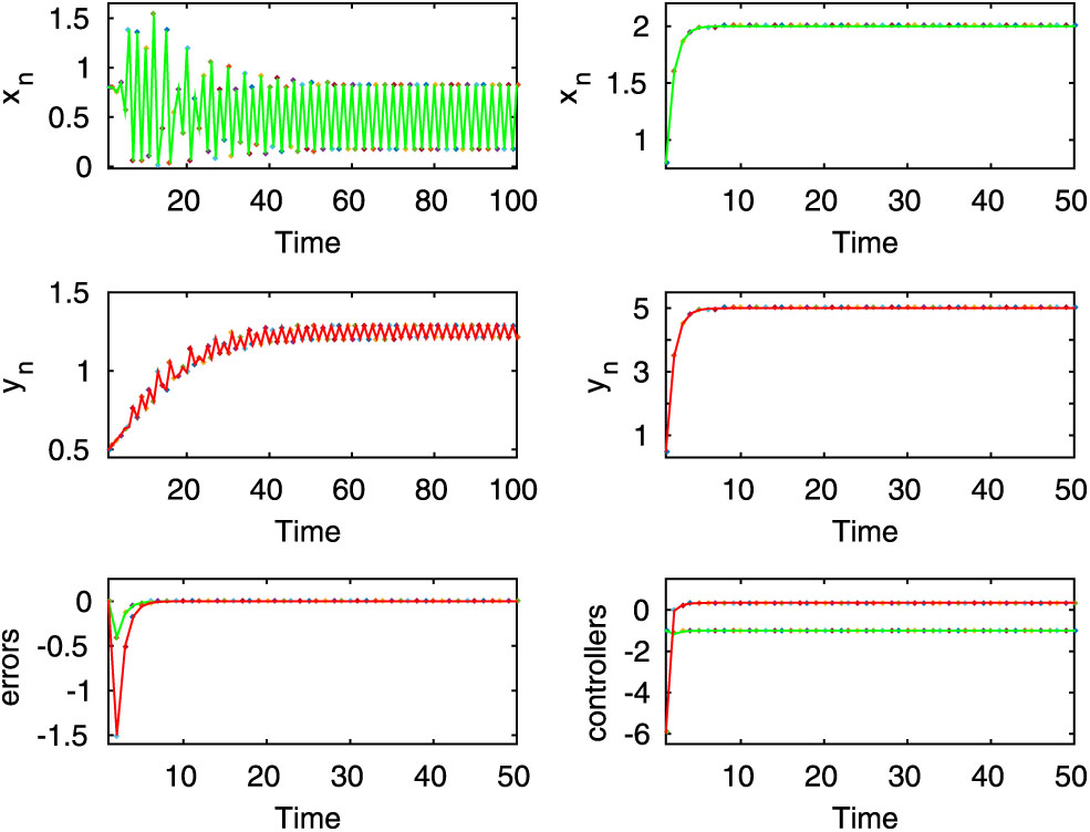
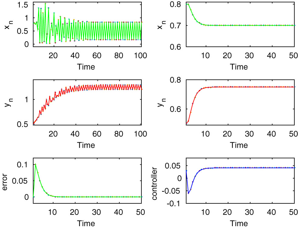
Here, the first two rows of left column exhibit periodic oscillation for the uncontrolled system (2.8), whereas the first two rows of the right column show stable dynamics of the controlled system (2.9). Here,
Here, both uncontrolled and controlled systems exhibit stable dynamics, which are shown in the first two rows for
3 Indirect control of population
In this section, the design procedure of indirect Z-control laws for a discrete-time system is discussed. Here we intend to control the prey population density by taking control measure on the predator population and applying indirect Z-type control mechanism. Also, this section provides theoretical analysis to show the effectiveness of indirect Z-type control law.
3.1 Controller design
Here, we apply indirect Z-type control on the predator–prey model (2.8). For this purpose we introduce an exogenous measure on the predator population and then the model (2.8) takes the following form:
where,
Now, our aim is to find the analytical expression of the indirect control variable
For this, first we define an error function as
Next we consider the design formula as
where,
but equation (3.4) does not contain
and the behavior of
Using
Now putting the value of
After that substituting the value of
and finally we obtain the control variable as
where
Here equation (3.9) gives the indirect controller for the controlled system (3.1).
Therefore, using the error function and the design formula we obtain the analytical expression for input
3.2 Theoretical analysis
In this subsection, the convergence performance of the Z-type controller (3.9) for the model (3.1) is examined theoretically. Here, we show that the error for the model (3.1) equipped with indirect Z-controller converges to zero.
Theorem 2:
For a bounded desired state
Proof: According to the design procedure of Z-type controller (3.9), we obtain that
Now, substituting (3.11) into
Solving the above difference equation (3.12) we get
where
Using the initial condition, we obtain
Therefore, the tracking error
3.3 Numerical simulation
In this subsection, numerical simulations are offered to verify the success of the indirect Z-type controller (3.9). Here, we consider the same parameter values and initial conditions as taken in subsection 2.4. In a similar manner, as described in the direct case, we choose the value of the parameter r in such a way that the system (2.8) without Z-control shows chaotic, periodic and stable dynamics respectively. Then we apply indirect Z-type controller on the predator population for controlling the prey population density. Here we choose the value of the design parameter
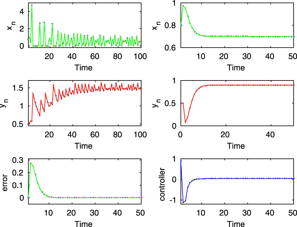
Here, the first two rows of left column show chaotic dynamics of the uncontrolled system (2.8) for
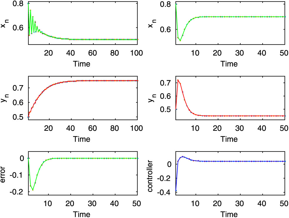
Here, both the controlled and uncontrolled systems show stable dynamics, which are executed in the first two rows of first and second column for
Now we draw the basin of attractions of the controlled system (3.1) for two different values of the design parameter m (2 and 2.5), with desired prey population density
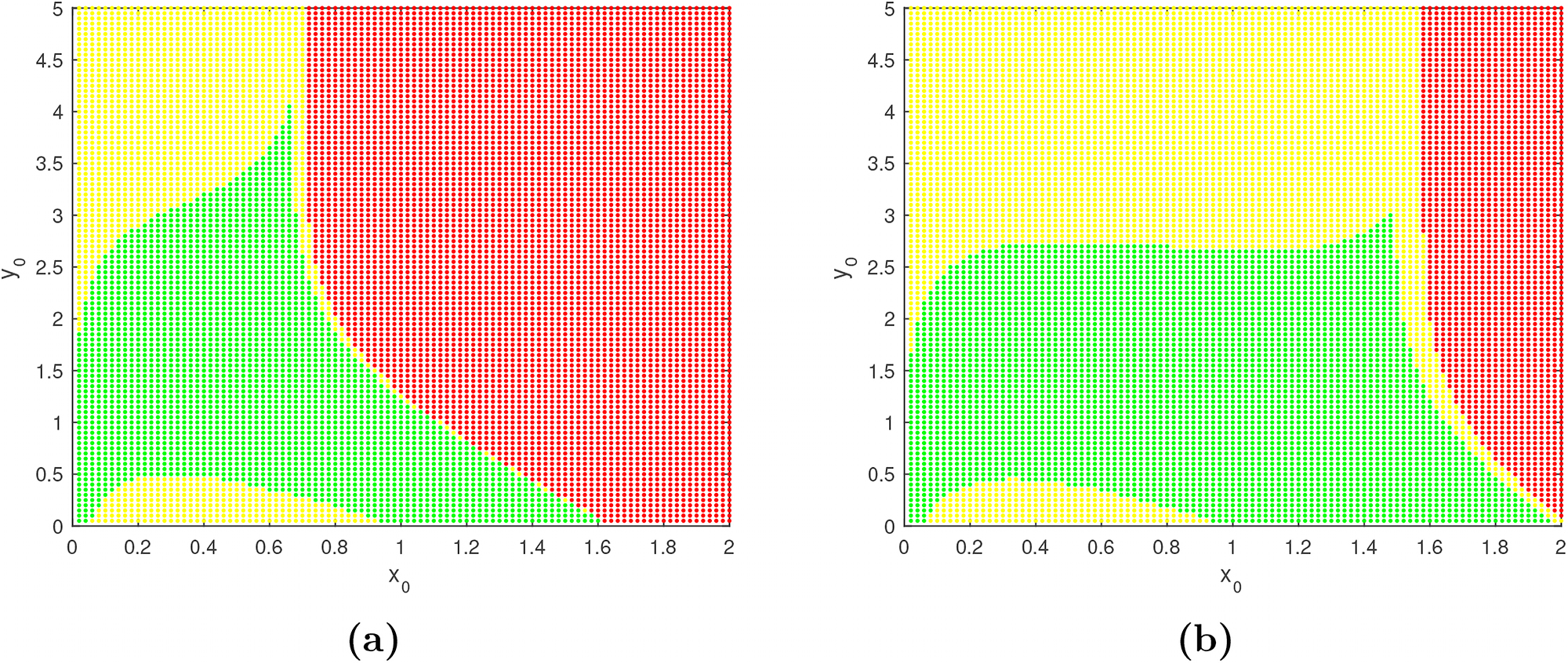
Figure shows the basin of attraction of the Z-controlled system (3.1) for two different values of the design parameter m. Here, in the left figure
For a better interpretation of these phenomena, we select different initial conditions
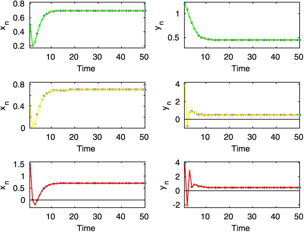
Here, from the first row it is seen that both prey and predator populations remain at positive level for the initial state
3.3.1 Application of indirect Z-controller for a periodic desired state
The controller (3.9) is also capable to drive the prey population to a periodic desired state whereas the uncontrolled system shows chaotic, periodic, and stable dynamics respectively. For the successful execution of these phenomena, we consider the parameter values and the initial state same as subsection 2.4. We also choose the periodic desired states of the prey population as
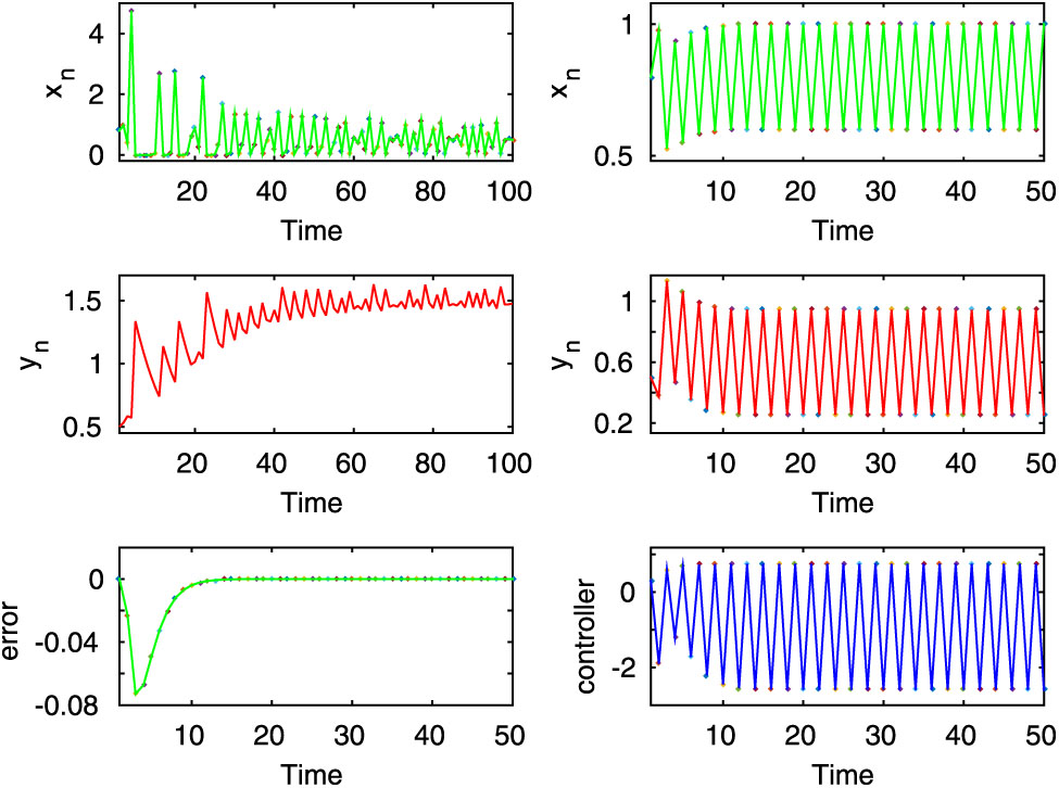
In this figure, the first two rows of left column show the chaotic dynamics for the uncontrolled system (2.8) for
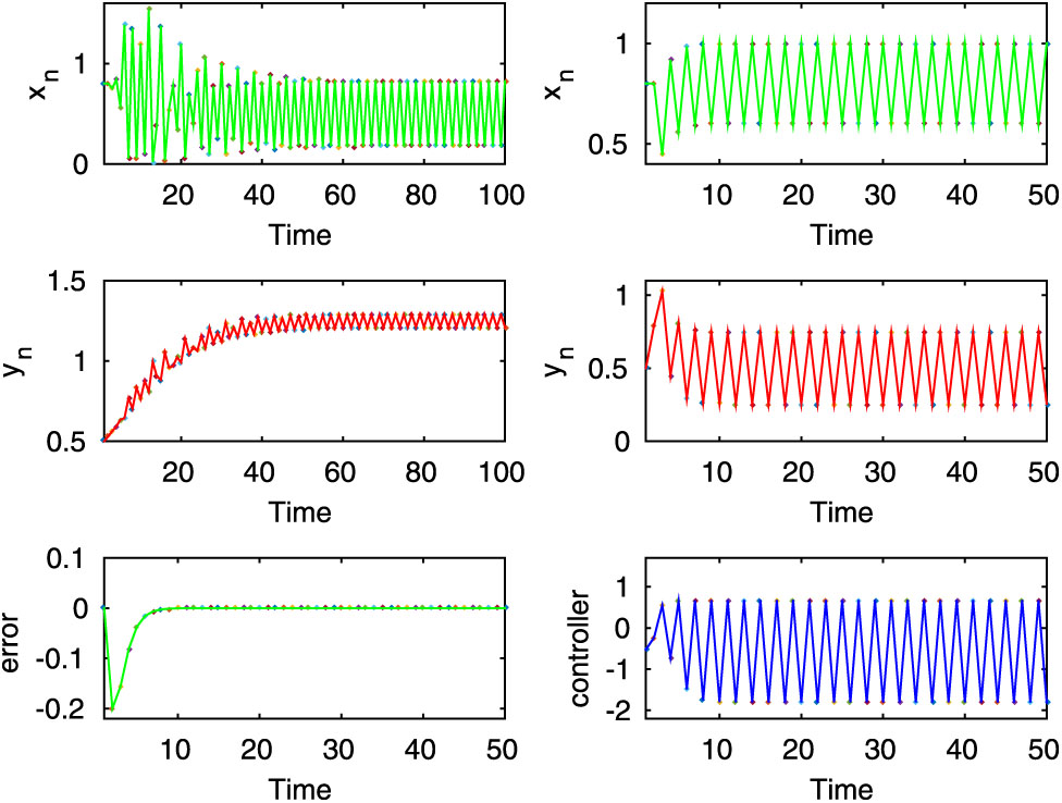
Here, from the first two rows, it is seen that both uncontrolled and controlled systems show periodic oscillations for
Here, the first two rows of left column show stable dynamics of the uncontrolled system (2.8), on the other hand, from the first two rows of right column it is observed that the desired state of prey population of the controlled system (3.1) is periodic for
4 Conclusion
In the real-world, all species are important to maintain the ecological balance, and they interact with each other and also with their environment in an elegantly balanced cycle. But as time goes, ecological imbalance increases due to the excessive growth of some species, sudden death of some species, careless human activities, changing climate, habitat loss, degradation, etc., for which negative consequences occur in the ecosystem. But for the survival of all species in the world, preservation of ecological balance is very important and it will be maintained if all the species are in the desired states. So it is sometimes needed to control the population of a system to a reasonable level, because either this population drives others to become extinct or even itself becomes extinct. According to top-down control, predator plays an important role in controlling the prey population size and community structure in a food web ecology. However, a pre-defined prey population abundance may not be achieved only through top-down control. It can be done successfully by applying Z-type controller, which is a combination of immigration, emigration, culling, and harvesting.
To investigate the effectiveness of Z-type control mechanism in a discrete-time predator–prey system, we have considered a Lotka–Volterra type predator–prey model with direct and indirect Z-control laws in discrete-time set-up. We observed that in both direct and indirect cases the Z-type controller group (2.10) (for prey and predator species) and the controller (3.9) (for the prey species) drive the populations to the respective desired states. It is also investigated that the controller is able to keep species far from the risk of disappearance i.e. the species do not die out from the environment. Here, the time-series evaluation of the update parameters (or parameter) has great importance. We have observed that the update parameters can take both positive and negative values for achieving the desired population density. In both the direct and indirect Z-control mechanisms, the positive value of the update parameter implies the removal of a population from the system through emigration, harvesting, or culling, whereas the negative value of the update parameter implies the addition of population into the system through immigration. In the Z-type control mechanism, we can change the prey and predator population densities or predator population density through emigration, immigration, culling, or harvesting to obtain the desired dynamics. For direct control, addition or removal of a certain amount of prey and predator species (for indirect control, addition, or removal of a certain amount of predator species) stabilize the system. Now it is worthy to note that the rate at which the species should be added into or removed from the system to achieve the desired state and it is quantified by the magnitude of the update parameter. Also, we have observed that for any value of the design parameter
We can conclude that such an error-based dynamic method (Z-type control) plays an important role for maintaining the ecological balance. Riechert et al. [46] experimentally showed that when spiders are added in the vegetable system, then the number of pests significantly decline and the amount of average damage reduced to 31.8% from 93.3%. Therefore, predators limit associated prey populations. The above experimental results can be implemented in an ecosystem most effectively by using Z-control mechanism. This error based Z-control mechanism is very useful for serving ecosystems, via, stabilizing the unstable equilibrium point, originating new stable equilibrium point or shifting the population oscillation away from zero. Therefore, Z-type control mechanism can be considered as a control mechanism that can be applied for conservation biology and strategic management of pest control in an ecological system.
Acknowledgments
The authors are thankful to the two anonymous reviewers and the handling editor for their valuable comments and suggestions, which helped us to improve the paper.
-
Research funding: None declared.
-
Author contribution: All the authors have accepted responsibility for the entire content of this submitted manuscript and approved submission.
-
Conflict of interest statement: The authors declare no conflicts of interest regarding this article.
References
[1] E. J. Kormondy, Concepts of Ecology, Englewood Cliffs, New Jersey, Prentice-Hall, 1969.10.2307/3543229Suche in Google Scholar
[2] P. J. Morin, Community Ecology, Oxford, Blackwell Science, 1999.Suche in Google Scholar
[3] T. M. Smith, R. L. Smith, and I. Waters, Elements of Ecology, San Francisco, Benjamin-Cummings, 2012.Suche in Google Scholar
[4] M. L. Cain, W. D. Bowman, and S. D. Hacker, Ecology, ed, Sunderland, Mass, Sinauer, 2008.Suche in Google Scholar
[5] M. R. Evans, “Modelling ecological systems in a changing world,” Phil. Trans. Biol. Sci., vol. 367, no. 1586, pp. 181–190, 2012, https://doi.org/10.1098/rstb.2011.0172.Suche in Google Scholar PubMed PubMed Central
[6] R. K. Upadhyay and S. R. Iyengar, Introduction to Mathematical Modeling and Chaotic Dynamics, New York, CRC Press, 2013.10.1201/b15317Suche in Google Scholar
[7] G. C. Layek, An Introduction to Dynamical Systems and Chaos, New Delhi, Springer, 2015.10.1007/978-81-322-2556-0Suche in Google Scholar
[8] S. Pal, N. Pal, and J. Chattopadhyay, “Hunting cooperation in a discrete-time predator–prey system,” Int. J. Bifurcat. Chaos, vol. 28, p. 1850083, 2018, https://doi.org/10.1142/S0218127418500839.Suche in Google Scholar
[9] R. M. May, “Biological populations with nonoverlapping generations: stable points, stable cycles, and chaos,” Science, vol. 186, no. 4164, pp. 645–647, 1974, https://doi.org/10.1126/science.186.4164.645.10.1126/science.186.4164.645Suche in Google Scholar PubMed
[10] J. D. Murray, Mathematical biology: I. An introduction, Berlin, Germany, Springer Science & Business Media, 2007.Suche in Google Scholar
[11] T. Peter and A. D. Taylor, “Complex dynamics in ecological time series,” Ecology, vol. 73, pp. 289–305, 1992, https://doi.org/10.2307/1938740.Suche in Google Scholar
[12] R. F. Costantino, J. M. Cushing, B. Dennis, and R. A. Desharnais. Experimentally induced transitions in the dynamic behaviour of insect populations,” Nature, vol. 375, pp. 227–230, 1995, https://doi.org/10.1038/375227a0.Suche in Google Scholar
[13] A. Hastings and T. Powell, “Chaos in a three-species food chain,” Ecology, vol. 72, no. 3, pp. 896–903, 1991, https://doi.org/10.2307/1940591.Suche in Google Scholar
[14] J. M. Ginoux, R. Naeck, Y. B. Ruhomally, M. Z Dauhoo, and M. Perc, “Chaos in a predator–prey-based mathematical model for illicit drug consumption,” Appl. Comput. Math., vol. 347, pp. 502–513, 2019, https://doi.org/10.1016/j.amc.2018.10.089.Suche in Google Scholar
[15] H. Sayama, Introduction to the Modeling and Analysis of Complex Systems. Open SUNY Textbooks, Geneseo, Milne Library, State University of New York, 2015.Suche in Google Scholar
[16] T. R. Malthus, An Essay on the Principle of Population, New York, Dover Publications, 2007.Suche in Google Scholar
[17] A. J. Lotka, “Elements of physical biology,” Sci. Prog. Twent. Century (1919–1933), vol. 21, no. 82, pp. 341–343, 1926.Suche in Google Scholar
[18] V. Volterra, “Variations and fluctuations of the number of individuals in animal species living together,” ICES J. Mar. Sci., vol. 3, no. 1, pp. 3–51, 1928, https://doi.org/10.1093/icesjms/3.1.3.Suche in Google Scholar
[19] C. S. Holling, “The components of predation as revealed by a study of small-mammal predation of the european pine sawfly,” Can. Entomol., vol. 91, pp. 293–320, 1959, https://doi.org/10.4039/Ent91293-5.Suche in Google Scholar
[20] S. Pal, N. Pal, S. Samanta, and J. Chattopadhyay, “Effect of hunting cooperation and fear in a predator-prey model,” Ecol. Complex., vol. 39, p. 100770, 2019, https://doi.org/10.1016/j.ecocom.2019.100770.Suche in Google Scholar
[21] G. D. Ruxton, “Low levels of immigration between chaotic populations can reduce system extinctions by inducing asynchronous regular cycles,” Proc. R. Soc. Lond. B Biol. Sci., vol. 256, pp. 189–193, 1994, https://doi.org/10.1098/rspb.1994.0069.Suche in Google Scholar
[22] G. D. Ruxton, “Chaos in a three-species food chain with a lower bound on the bottom population,” Ecology, vol. 77, no. 1, pp. 317–319, 1996, https://doi.org/10.2307/2265680.Suche in Google Scholar
[23] J. N. Eisenberg and D. R. Maszle, “The structural stability of a three-species food chain model,” J. Theor. Biol., vol. 176, no. 4, pp. 501–510, 1995, https://doi.org/10.1006/jtbi.1995.0216.Suche in Google Scholar
[24] K. McCann and A. Hastings, “Re–evaluating the omnivory–stability relationship in food webs,” Proc. R. Soc. Lond. B Biol. Sci., vol. 264, pp. 1249–1254, 1997, https://doi.org/10.1098/rspb.1997.0172.Suche in Google Scholar
[25] C. L. Xu and Z. Z. Li, “Influence of intraspecific density dependence on a three-species food chain with and without external stochastic disturbances,” Ecol. Model., vol. 155, no. 1, pp. 71–83, 2002, https://doi.org/10.1016/S0304-3800(02)00067-4.Suche in Google Scholar
[26] J. Chattopadhyay and R. R. Sarkar, “Chaos to order: preliminary experiments with a population dynamics models of three trophic levels,” Ecol. Model., vol. 163, no. 1–2, pp. 45–50, 2003, https://doi.org/10.1016/S0304-3800(02)00381-2.Suche in Google Scholar
[27] D. O. Maionchi, S. F. Dos Reis, and A. M. De Aguiar, “Chaos and pattern formation in a spatial tritrophic food chain,” Ecol. Model., vol. 191, no. 2, pp. 291–303, 2006, https://doi.org/10.1016/j.ecolmodel.2005.04.028.Suche in Google Scholar
[28] V. A. Jansen and A. L. Lloyd, “Local stability analysis of spatially homogeneous solutions of multi-patch systems,” J. Math. Biol., vol. 41, no. 3, pp. 232–252, 2000, https://doi.org/10.1007/s002850000048.Suche in Google Scholar PubMed
[29] N. Pal, S. Samanta, and J. Chattopadhyay, “The impact of diffusive migration on ecosystem stability,” Chaos, Solit. Fractals, vol. 78, pp. 317–328, 2015, https://doi.org/10.1016/j.chaos.2015.08.011.Suche in Google Scholar
[30] N. Pal, S. Samanta, and S. Rana, “The impact of constant immigration on a tri-trophic food chain model,” Int. J. Appl. Comput. Math., vol. 3, no. 4, pp. 3615–3644, 2017, https://doi.org/10.1007/s40819-017-0317-5.Suche in Google Scholar
[31] N. Pal, S. Samanta, and J. Chattopadhyay, “Revisited hastings and powell model with omnivory and predator switching. Chaos,” Solit. Fractals, vol. 66, pp. 58–73, 2014, https://doi.org/10.1016/j.chaos.2014.05.003.Suche in Google Scholar
[32] J. Chattopadhyay, N. Pal, S. Samanta, E. Venturino, and Q. J. A. Khan, “Chaos control via feeding switching in an omnivory system,” Biosystems, vol. 138, pp. 18–24, 2015, https://doi.org/10.1016/j.biosystems.2015.10.006.Suche in Google Scholar PubMed
[33] S. Pal, S. K. Sasmal, and N. Pal, “Chaos control in a discrete-time predator–prey model with weak allee effect,” Int. J. Biomath., vol. 11, no. 7, p. 1850089, 2018, https://doi.org/10.1142/S1793524518500894.Suche in Google Scholar
[34] S. Gakkhar and A. Singh, “Control of chaos due to additional predator in the Hastings–Powell food chain model,” J. Math. Anal. Appl., vol. 385, no. 1, pp. 423–438, 2012, https://doi.org/10.1016/j.jmaa.2011.06.047.Suche in Google Scholar
[35] B. Sahoo and S. Poria, “The chaos and control of a food chain model supplying additional food to top-predator,” Chaos, Solit. Fractals, vol. 58, pp. 52–64, 2014, https://doi.org/10.1016/j.chaos.2013.11.008.Suche in Google Scholar
[36] B. Sahoo and S. Poria, “Effects of supplying alternative food in a predator–prey model with harvesting,” Appl. Math. Comput., vol. 234, pp. 150–166, 2014, https://doi.org/10.1016/j.amc.2014.02.039.Suche in Google Scholar
[37] P. Panday, N. Pal, S. Samanta, and J. Chattopadhyay, “Stability and bifurcation analysis of a three-species food chain model with fear,” Int. J. Bifurcat. Chaos, vol. 28, no. 1, p. 1850009, 2018.10.1142/S0218127418500098Suche in Google Scholar
[38] P. Panday, N. Pal, S. Samanta, and J. Chattopadhyay, “A three species food chain model with fear induced trophic cascade,” Int. J. Appl. Comput. Math., vol. 5, no. 4, 2019. https://doi.org/10.1007/s40819-019-0688-x.Suche in Google Scholar
[39] Y. Zhang, X. Yan, B. Liao, Y. Zhang, and Y. Ding, “Z-type control of populations for Lotka–Volterra model with exponential convergence,” Math. Biosci., vol. 272, pp. 15–23, 2016. https://doi.org/10.1016/j.mbs.2015.11.009.Suche in Google Scholar PubMed
[40] D. Lacitignola, F. Diele, C. Marangi, and A. Provenzale, “On the dynamics of a generalized predator–prey system with Z-type control,” Math. Biosci., vol. 280, pp. 10–23, 2016. https://doi.org/10.1016/j.mbs.2016.07.011.Suche in Google Scholar PubMed
[41] S. K. Shahid Nadim, S. Samanta, N. Pal, I. M. ELmojtaba, I. Mukhopadhyay, and J. Chattopadhyay, “Impact of predator signals on the stability of a predator–prey system: a Z-control approach,” Differ. Equ. Dyn. Syst., 2018, In press.Suche in Google Scholar
[42] A. K. Alzahrani, A. S. Alshomrani, N. Pal, and S. Samanta, “Study of an eco-epidemiological model with Z-type control,” Chaos, Solit. Fractals, vol. 113, pp. 197–208, 2018.10.1016/j.chaos.2018.06.012Suche in Google Scholar
[43] S. Samanta, “Study of an epidemic model with Z-type control,” Int. J. Biomath., vol. 11, no. 07, p. 1850084, 2018. https://doi.org/10.1142/S1793524518500845.Suche in Google Scholar
[44] D. Lacitignola and F. Diele, “On the Z-type control of backward bifurcations in epidemic models,” Math. Biosci., vol. 315, p. 108215, 2019. https://doi.org/10.1016/j.mbs.2019.108215.Suche in Google Scholar PubMed
[45] A. Senapati, P. Panday, S. Samanta, and J. Chattopadhyay, “Disease control through removal of population using z-control approach,” Physica A: Stat. Mechan. Appl., 2019. https://doi.org/10.1016/j.physa.2019.123846.Suche in Google Scholar PubMed PubMed Central
[46] S. E. Riechert and L. Bishop, “Prey control by an assemblage of generalist predators: spiders in garden test systems,” Ecology, vol. 71, no. 4, pp. 1441–1450, 1990. https://doi.org/10.2307/1938281.Suche in Google Scholar
© 2020 Shilpa Garai et al., published by De Gruyter, Berlin/Boston
This work is licensed under the Creative Commons Attribution-NonCommercial-NoDerivatives 4.0 International License.
Artikel in diesem Heft
- Frontmatter
- General
- Remote magnetically controlled drug release from electrospun composite nanofibers: design of a smart platform for therapy of psoriasis
- Dynamical Systems & Nonlinear Phenomena
- A modified simple chaotic hyperjerk circuit: coexisting bubbles of bifurcation and mixed-mode bursting oscillations
- Dynamics of a discrete-time system with Z-type control
- Dynamic response of axially loaded end-bearing rectangular closed diaphragm walls
- Hydrodynamics
- Admissibility conditions for Riemann data in shallow water theory
- Numerical study on the rotating electro-osmotic flow of third grade fluid with slip boundary condition
- Solid State Physics & Materials Science
- Ultrasonic study of Si-oil based magneto-rheological fluid
- Electromagnetic propagation characteristics of one-dimensional photonic crystals with metal layers in quasi-parity-time (PT)-symmetric system
- Thermodynamics & Statistical Physics
- Combined influence of axial electron temperature and exponential plasma density ramp on the self-focusing of a chirped laser in plasma