Solving Fractional Partial Differential Equations with Variable Coefficients by the Reconstruction of Variational Iteration Method
-
Esmail Hesameddini
 und
Azam Rahimi
und
Azam Rahimi

Abstract
In this article, we propose a new approach for solving fractional partial differential equations with variable coefficients, which is very effective and can also be applied to other types of differential equations. The main advantage of the method lies in its flexibility for obtaining the approximate solutions of time fractional and space fractional equations. The fractional derivatives are described based on the Caputo sense. Our method contains an iterative formula that can provide rapidly convergent successive approximations of the exact solution if such a closed form solution exists. Several examples are given, and the numerical results are shown to demonstrate the efficiency of the newly proposed method.
1 Introduction
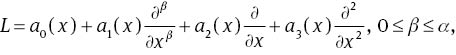
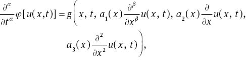
Fractional differential equations are generalised form of integer order ones, which are achieved by replacing the integer order derivatives by fractional ones. Compared with integer order differential equations, fractional differential equations are more capable for simulating natural physical process and dynamic system [1, 2]. Fractional calculus has become the focus of interest for many researchers in different fields of science and engineering. A lot of research has shown the advantages of using the fractional calculus in the modelling and control of many dynamical systems [3, 4]. Many physics and engineering systems can be elegantly modeled with the help of the fractional derivative, such as dielectric polarisation [5], electrolyte–electrolyte polarisation [6] and viscoelastic systems [7]. Owing to the increasing applications, there has been important interest in developing numerical methods for the solution of fractional differential equations. These methods include Adomian decomposition method (ADM) [8], generalised differential transform method [9], variational iteration method (VIM) [10], finite difference method [11], homotopy analysis method [12] and wavelet method [13]. In this article, our study focuses are on the fractional partial differential equations (FPDEs). FPDEs are generalisations of classical partial differential equations, and they can be classified into three principal kinds: space-time fractional differential equation, space-fractional differential equation and time-fractional differential equation. One of the simplest examples of the former is fractional order diffusion equations, which are generalisations of classical diffusion equations. In the present article, we consider the following FPDE with variable coefficients:
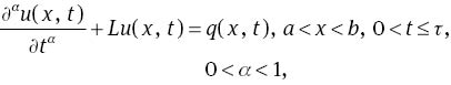
where L is the linear operator
subject to the initial condition

where ∂α/∂tα and ∂β/∂xβ are fractional derivatives of the Caputo sense, ai(x) for i=0, …, 3 and q(x, t) are known continuous functions and u(x, t) is the unknown function. The analytic results on existence and uniqueness of solutions to fractional differential equations have been investigated by many authors, see, say for example [14]. Uddin and Haq [15] used radial basis functions for the solution of (1) with constant coefficients. Also, Garrappa and Popolizio [16] used the matrix functions for solving this problem. We construct the solution of problem (1–3) using the reconstruction of variational iteration method (RVIM). The RVIM was first suggested by Hesameddini and Latifizadeh for solving ordinary differential equations (ODE) [17]. In this work, we extend this method to solve FPDEs. It does not only simplify the problem but also speeds up the computation. Our method contains an iterative formula that can provide rapidly convergent successive approximations of the exact solution if such a closed-form solution exists. The rest of this article is as follows. In Section 2, some preliminaries are presented that will be used in later sections. In Section 3, the method is discussed. In Section 4, study on the convergence of this method is illustrated. Section 5 is devoted to numerical experiments, and the results are compared with the exact solutions and some previous works. Section 6 is the conclusion.
2 Preliminaries
For the reader’s convenience, we present some necessary definitions that are used further in this article.
Definition 1 A real function f(t), t>0, is said to be in the space Cμ, μ∈R if there exists a real number p(>μ), such that f(t)=tpv(t), where v(t)∈C[0, ∞), and it is said to be in the space
Definition 2 The Riemann–Liouville fractional integral operator of order α ≥ 0, of a function f(t)∈Cμ, μ ≥ −1, is defined as
such that J0f(t)=f(t). Note that Γ is the gamma function [14].
Definition 3 For a continuous function f(t), the Caputo fractional partial derivative of order α, where n − 1<α<n, is defined as [18]
Definition 4 The Laplace transform of the Caputo fractional derivative ∂αu(x, t)/∂tα is given by
where U(x, s)=ℓ{u(x, t); s}, n − 1 ≤ α<n.
3 Implementation of the Method
To illustrate the basic idea of our technique, we rewrite the general problem (1–3) as follows:
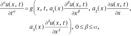
where
with the initial conditions

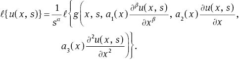
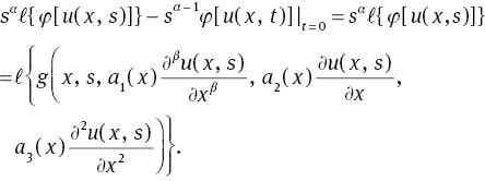
By taking the Laplace transform on both sides of (4), in the usual way and using the zero artificial initial conditions, the following result is obtained:
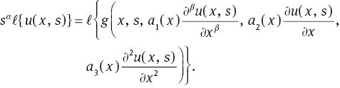
Therefore, we can conclude that
Suppose that 1/sα=H(s), then by using the convolution theorem, one obtains
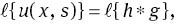
where ℓ−1{H(s)}=h(t). Taking the inverse Laplace transform to both sides of (7), the result is as follows:
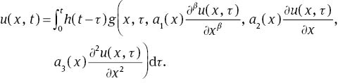
Now, we must impose the actual initial conditions to obtain the solution of (4). Thus, the following iteration formulation is resulted:
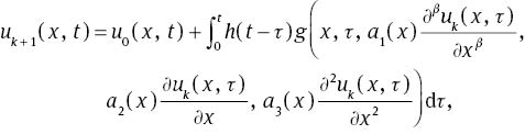
where the value of u0(x, t) is obtained by the actual initial conditions (5) and satisfied in
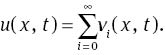
The RVIM assumes a series solution for u(x, t) by an infinite sum of components u(x, t)=limk→∞uk(x, t).
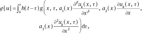
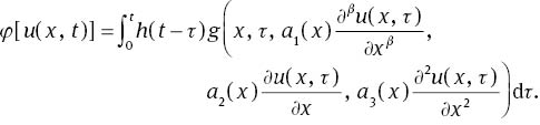
Now, define the operator φ[u] as
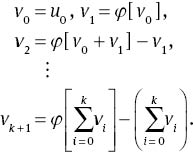
and also the components vk, k=0, 1, … as the following:
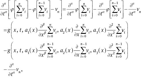
Using the relations of (10), (12) and (13), result in
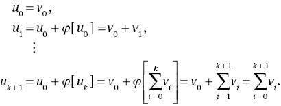
Then, consequently, we have
Corollary 1If 0<α<1, then
where the operatorφ[u] is defined in (12).
Proof. For clarifying the corollary, it is sufficient to take the Laplace transform of both sides of (16), then we have
Suppose that 1/sα=H(s) and ℓ−1{H(s)}=h(t), then by taking the inverse Laplace transform from both sides of (17), one obtains
Therefore, according to the definition of the operator φ[u], the proof is complete.
4 Study on the Convergence of Method
In this section, according to the approach that is proposed in the pervious section, the sufficient conditions for convergence of the method and the error estimate are presented. The main results are proposed in the following theorems.
Theorem 1Let φ, defined in (12), be an operator from a Hilbert space H to H. The series solution
Proof. Define a sequence
We show that

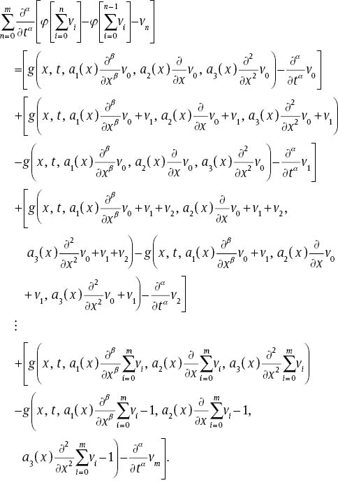
For every n, m∈N, n ≥ m, we have
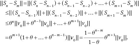
Since 0<θ<1, we get limm,n→||Sn − Sm||=0. Therefore,
Theorem 2If the series solution given by (15) converges, then it is an exact solution of the FPDE with variable coefficients (4).
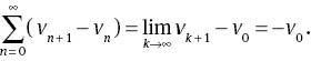
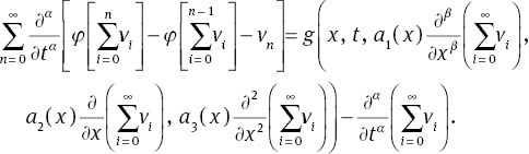
Proof. Suppose that the series solution (15) converges, then we have
Also,
Applying the linear operator ∂α/∂tα to both sides of (21) and according to relations (11) and (13), we obtain
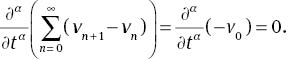
On the other hand, definition (12) implies
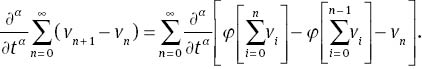
For n>1, using Corollary 1, one obtains
also for n=0, we have
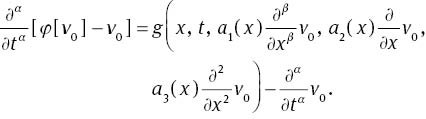
Now substituting relations (24) and (25) in (23), result in
Therefore,
From (22), (23) and (27), we can observe that
Theorem 3If the series solution
Proof. Theorem 1 and inequality (20) imply that
Now, if n→∞, we have Sn→u(x, t). So,
Also, since 0<θ<1, we have (1 − θ(n–m)) ≤ 1. Therefore, the preceding inequality becomes
In summary, Theorems 1 and 2 indicate that the solution of the problem (4) is obtained by using the iteration formula (10). This approximate formula converges to its exact solution under the condition of existing 0<θ<1 such that
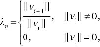
then the series solution
where λ=max{λi, i=0, 1, …, m}.
5.1 Numerical Examples
In this section, we apply the proposed approach of RVIM to solve some FPDEs with variable coefficients. We also examine the conditions for convergent RVIM solution of these problems to their exact solutions.
Example 1Consider the following fractional heat-like equation
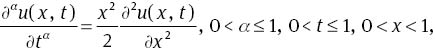
subject to the initial condition
The exact solution is
To obtain the RVIM solution, we apply the Laplace transform on both sides of (31)
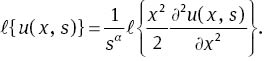
Applying the inverse Laplace transform to both sides of (33), result in
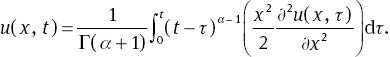
Considering the initial condition (32), the following iterative relation is obtained
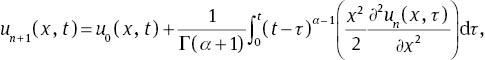
where u0(x, t)=x2 and un(x, t) indicate the nth approximation of u(x, t). So, φ[u] is defined as
According to (36) and (13), after some simplification and substitution, the following relations are resulted:
therefore, the solution of (31) will be obtained as

For the approximation purpose, we approximate the solution u(x, t) by the nth-order truncated series
that leads to its exact solution, where Eα(z) is the one parameter Mittag–Leffler function defined by [19]
By using this method, the exact solution of the problem is obtained. To illustrate the effectiveness of our method, we compare it to other numerical methods. For α=0.75, 0.9 and α=1, a comparison between our method and the other methods such as VIM, ADM and Sinc–Legendre collocation method [20] is demonstrated in Tables 1–3. Also, Figure 1 shows the comparison between the absolute error function |u(x, t)|−un(x, t)|, which is obtained by the presented method with n=10, α=1 and Sinc–Legendre collocation method. This figure shows that our method can provide more accurate solution than the Sinc–Legendre collocation method [20]. Also, Table 3 shows that our method is clearly reliable if it is compared with the other mentioned methods. In addition, the λi for this problem will be obtained as
Comparison of the RVIM solution with other methods for α=0.75 in Example 1.
| t | x | VIM | ADM | Sinc–Legendre (m=15) | Presented method |
|---|---|---|---|---|---|
| 0.25 | 0.3 | 1.293e-01 | 1.346e-01 | 1.312e-01 | 1.349e-01 |
| 0.6 | 5.175e-01 | 5.385e-01 | 4.957e-01 | 5.396e-01 | |
| 0.9 | 1.164e-00 | 1.211e-00 | 1.055e-01 | 1.214e-00 | |
| 0.50 | 0.3 | 1.695e-01 | 1.795e-01 | 1.685e-01 | 1.819e-01 |
| 0.6 | 6.780e-01 | 7.183e-01 | 6.303e-01 | 7.278e-01 | |
| 0.9 | 1.525e-00 | 1.616e-00 | 1.352e-00 | 1.638e-00 | |
| 0.75 | 0.3 | 2.154e-01 | 2.313e-01 | 2.118e-01 | 2.402e-01 |
| 0.6 | 8.618e-01 | 9.255e-01 | 7.962e-01 | 9.606e-01 | |
| 0.9 | 1.939e-00 | 2.082e-00 | 1.733e-00 | 2.161e-00 | |
| 1.00 | 0.3 | 2.687e-01 | 2.909e-01 | 2.645e-01 | 3.137e-01 |
| 0.6 | 1.075e-00 | 1.163e-00 | 9.745e-01 | 1.255e-00 | |
| 0.9 | 2.419e-00 | 2.618e-00 | 2.014e-00 | 2.823e-00 |
Comparison of the RVIM solution with other methods for α=0.9 in Example 1.
| t | x | VIM | ADM | Sinc–Legendre (m=15) | Presented method |
|---|---|---|---|---|---|
| 0.25 | 0.3 | 1.210e-01 | 1.218e-01 | 1.212e-01 | 1.219e-01 |
| 0.6 | 4.841e-01 | 4.872e-01 | 4.762e-01 | 4.874e-01 | |
| 0.9 | 1.089e-00 | 1.096e-00 | 1.046e-00 | 1.097e-00 | |
| 0.50 | 0.3 | 1.567e-01 | 1.588e-01 | 1.564e-01 | 1.595e-01 |
| 0.6 | 6.268e-01 | 6.355e-01 | 6.086e-01 | 6.381e-01 | |
| 0.9 | 1.410e-00 | 1.429e-00 | 1.342e-00 | 1.436e-00 | |
| 0.75 | 0.3 | 1.998e-01 | 2.041e-01 | 1.994e-01 | 2.071e-01 |
| 0.6 | 7.992e-01 | 8.165e-01 | 7.761e-01 | 8.284e-01 | |
| 0.9 | 1.798e-00 | 1.837e-00 | 1.722e-00 | 1.864e-00 | |
| 1.00 | 0.3 | 2.517e-01 | 2.588e-01 | 2.529e-01 | 2.677e-01 |
| 0.6 | 1.007e-00 | 1.035e-00 | 9.938e-01 | 1.071e-00 | |
| 0.9 | 2.265e-00 | 2.329e-00 | 2.144e-00 | 2.410e-00 |
Comparison of the absolute error for α=1 in Example 1.
| t | x | VIM and ADM | Sinc–Legendre (m=25) | Presented method |
|---|---|---|---|---|
| 0.25 | 0.3 | 1.54e-05 | 9.92e-08 | 0 |
| 0.6 | 6.16e-05 | 2.70e-06 | 0 | |
| 0.9 | 1.38e-04 | 1.02e-05 | 0 | |
| 0.50 | 0.3 | 2.60e-04 | 5.56e-07 | 0 |
| 0.6 | 1.03e-03 | 4.87e-06 | 1.00e-10 | |
| 0.9 | 2.34e-03 | 1.30e-05 | 0 | |
| 0.75 | 0.3 | 1.39e-03 | 1.14e-06 | 1.00e-10 |
| 0.6 | 5.56e-03 | 6.90e-06 | 4.00e-10 | |
| 0.9 | 1.25e-02 | 1.59e-05 | 0 | |
| 1.00 | 0.3 | 4.64e-03 | 9.83e-07 | 2.50e-9 |
| 0.6 | 1.85e-02 | 6.40e-06 | 9.8e-9 | |
| 0.9 | 4.18e-02 | 2.58e-05 | 2.2e-8 |
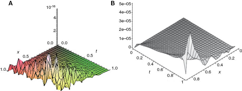
Graphs of the resulting absolute error, left (RVIM) and right (Sinc–Legendre), for α=1, in Example 1.
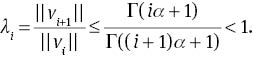
Figure 2 shows that the relation (39) is correct for i ≥ 10. This confirms that the reconstruction of variational approach for problem (31) converges to its exact solution.
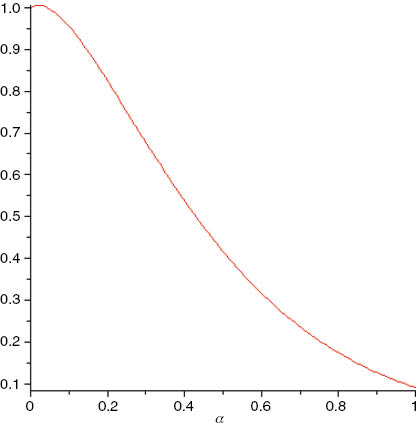
Plot of the function Γ(iα + 1)/Γ((i + 1)α + 1) with i=10.
Example 2Consider the following FPDE of order 0<α<1
subject to the initial condition

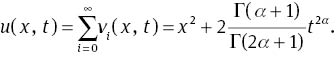
The exact solution of this problem is u(x, t) = x2 + 2(Γ(α + 1)/Γ(2α+1))t2α [21, 22].
According to RVIM, the recursive relation is given by
Thus, φ[u] is defined as
Using (13) and (43), the components vi can be obtained as follows:
Therefore, the exact solutions is
Furthermore, λi=||vi+ 1||/||vi||=0<1 for i ≥ 1. This confirms that the reconstruction of variational approach for FPDE (40) converges to its exact solution.
Figure 3 shows that the solution of this problem for α=0.6, which is obtained by the presented method, is the same as its exact solution.
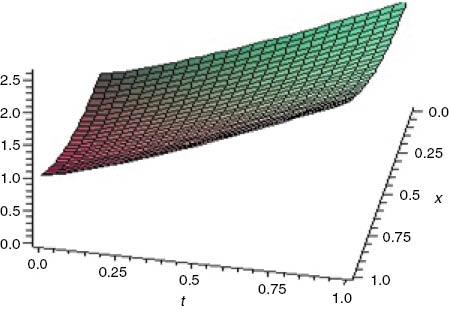
Plot of the RVIM solution for α=0.6 in Example 2.
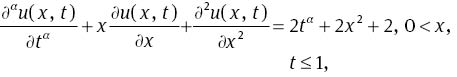
Example 3 Finally, consider the following FPDE
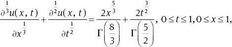
subject to the initial condition u(x, 0)=x2.
The exact solution of this problem is u(x, t)=x2 + t2 [23].
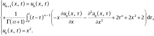
According to the RVIM, the recursive relation is given by
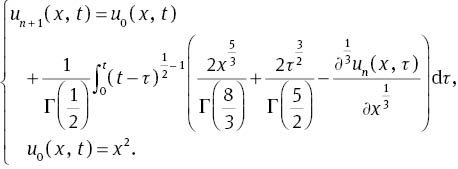
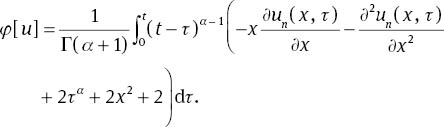
Thus, φ[u] is defined as
Using (13) and (47), the components vi can be obtained as follows:
Therefore, the exact solutions is
Furthermore, λi=||vi+ 1||/||vi||=0<1 for i ≥ 1 for i ≥ 2. This implies that the results of reconstruction of variational method for FPDE (45) converge to its exact solution and they confirm the efficiency of our method for solving these types of differential equations.
6 Conclusion
In this work, FPDEs with variable coefficients are handled by the RVIM. The convergence of the proposed method is proved through some theorems. Some examples are presented to show the validity and efficiency of our method. Also, we have examined the conditions for convergence of RVIM for these problems. From the computational point of view, the solutions obtained by our method are in excellent agreement with those obtained via previous works and also it is in very good coincidence with the exact solution. The results revealed that the RVIM method is an effective and powerful mathematical tool for solving FPDEs.
References
[1] S. A. EI-Wakil, A. Elhanbaly, and M. A. Abdou, Appl. Math. Comput. 182, 313 (2006).Suche in Google Scholar
[2] S. Chen and F. Liu, Appl. Math. Model. 33, 256 (2009).Suche in Google Scholar
[3] A. Calderon and B. Vinagre, Signal Process. 86, 2803 (2006).Suche in Google Scholar
[4] M. Tavazoei and M. Haeri, Phys. Lett. A 372, 798 (2008).10.1016/j.physleta.2007.08.040Suche in Google Scholar
[5] H. H. Sun, A. A. Abdelwahad, and B. Onaral, IEEE T. Automat. Contr. 29, 441 (1984).Suche in Google Scholar
[6] M. Ichise, Y. Nagayanagi, and T. Kojima, J. Electroanal. Chem. 33, 253 (1971).Suche in Google Scholar
[7] R. C. Koeller, J. Appl. Mech. 51, 299 (1984).Suche in Google Scholar
[8] I. L. EI-Kalla, Appl. Math. Comput. 21, 372 (2008).Suche in Google Scholar
[9] M. Dehghan, S. A. Yousefi, and A. Lotfi, Int. J. Numer. Meth. Biomed. Eng. 27, 467 (2011).Suche in Google Scholar
[10] Z. Odibat, Math. Comput. Model. 51, 1181 (2010).Suche in Google Scholar
[11] H. Sun, W. Chen, C. Li, Y. Chen, Int. J. Bifurcat. Chaos. 4, 22 (2012).Suche in Google Scholar
[12] I. Hashim and O. Abdulaziz, Commun. Nonlinear Sci. 3, 14 (2009).Suche in Google Scholar
[13] Y. M. Chen, M. X. Yi, and C. X. Yu, J. Comput. Sci. 3, 5 (2012).10.1016/j.jocs.2012.04.008Suche in Google Scholar
[14] A. A. Kilbas, H. M. Srivastava, and J. J. Trujillo, Theory and Applications of Fractional Differential Equations, Elsevier, San Diego 2006.Suche in Google Scholar
[15] M. Uddin and S. Haq, Commun. Nonlinear Sci. 21, 4208 (2011).Suche in Google Scholar
[16] R. Garrappa and M. Popolizio, Math. Comput. Simulat. 81, 1045 (2011).Suche in Google Scholar
[17] E. Hesameddini and H. Latifizadeh, Int. J. Nonlin. Sci. Num. 10, 1365 (2009).Suche in Google Scholar
[18] K. B. Oldham and J. Spanier, The Fractional Calculus: Theory and Application of Differentiation and Integration to Arbitrary Order, Academic Press, New York 1974.Suche in Google Scholar
[19] I. Podlubny, Fractional Differential Equations, Academic Press, New York 1999.Suche in Google Scholar
[20] A. Saadatmandi, M. Dehghan, and M. R. Azizi, Commun. Nonlinear Sci. 17, 4125 (2012).Suche in Google Scholar
[21] Z. Odibat and S. Momani, Appl. Math. Lett. 21, 194 (2008).Suche in Google Scholar
[22] Y. Chen, Y. Wu, Y. Cui, Z. Wang, and D. Jin, J. Comput. Sci. 1, 194 (2010).Suche in Google Scholar
[23] L. Wang, Y. Ma, and Z. Meng, Appl. Math. Comput. 227, 66 (2014).Suche in Google Scholar
©2015 by De Gruyter
Artikel in diesem Heft
- Frontmatter
- Spectrum and Green’s Function of a Many-Interval Sturm–Liouville Problem
- On a (3+1)-dimensional Boiti–Leon–Manna–Pempinelli Equation
- Inclined Magnetic Field Effect in Stratified Stagnation Point Flow Over an Inclined Cylinder
- Interaction between Barium Oxide and Barium Containing Chloride Melt
- Boundary-Layer Flow of Walters’ B Fluid with Newtonian Heating
- A Class of Boundary Value Problems Arising in Mathematical Physics: A Green’s Function Fixed-point Iteration Method
- Flow and Heat Transfer of Nanofluids Over a Rotating Porous Disk with Velocity Slip and Temperature Jump
- Soliton Solutions, Bäcklund Transformation and Lax Pair for Coupled Burgers System via Bell Polynomials
- Higher-Order Rogue Waves for a Fifth-Order Dispersive Nonlinear Schrödinger Equation in an Optical Fibre
- Solving Fractional Partial Differential Equations with Variable Coefficients by the Reconstruction of Variational Iteration Method
- A Direct Comparison between the Negative and Positive Effects of Throughflow on the Thermal Convection in an Anisotropy and Symmetry Porous Medium
- Corrigendum
- Corrigendum to: Kaluza-Klein Cosmological Model, Strange Quark Matter, and Time-Varying Lambda