A Direct Comparison between the Negative and Positive Effects of Throughflow on the Thermal Convection in an Anisotropy and Symmetry Porous Medium
-
Akil J. Harfash
 and
Ahmed K. Alshara
and
Ahmed K. Alshara

Abstract
The linear and nonlinear stability analysis of the motionless state (conduction solution) and of a vertical throughflow in an anisotropic porous medium are tested. In particular, the effect of a nonhomogeneous porosity and a constant anisotropic thermal diffusivity have been taken into account. Then, the accuracy of the linear instability thresholds are tested using a three dimensional simulation. It is shown that the strong stabilising effect of gravity field. Moreover, the results support the assertion that the linear theory, in general, is accurate in predicting the onset of convective motion, and thus, regions of stability.
1 Introduction
Penetrative convection refers to convective motion beginning in an unstable layer and penetrating into an otherwise stable layer or layers. Penetrative convection can be described in several ways, at least five of which are discussed in detail by Straughan [1]. One of the most widely employed models is internal heating, whereby an internal heat source (or sink) can cause a situation in which one part of a layer convects naturally while the other remains stable; so, penetrative convection can take place. Many references can be found describing convection via internal heating. One of the most significant of these has contributed greatly to progress in the research, that by Roberts [2], who developed a model of convection in a horizontal layer of fluid cooled from above, thermally insulated from below, and uniformly heated by an internal source. Matthews [3] reviewed Roberts’ work and developed a model for the onset of penetrative convection in a layer of fluid. A similar model of penetrative convection in a porous layer has been produced (see [4]). Mathematical models of penetrative convection, based on either an internal heat source or sink or using a nonlinear density–temperature relationship in the buoyancy term have been produced and rigorously analysed. Especially noteworthy are recent studies of linear instability and of nonlinear stability which are developed in other studies [5–8]. Further applications for some convection models have been developed and analysed [9–15].
Thermal convection in porous media has received considerable interest owing to many real-life applications ([16] and the references therein). Therefore, many studies have been developed to study the solution of convection in porous media analytically and numerically. Abbasbandy et al. [17] give a series solution for a steady flow of a third-grade fluid between two porous walls by the homotopy analysis method (HAM). Hayata et al. [18] introduce an analysis for model of flow and heat transfer characteristics in a third-grade fluid between two porous plates. In this study, the electrically conducting fluid fills the porous medium, and the solutions have been developed for small porosity and magnetic fields.
The literature on the study of the effect of vertical throughflow on convective instability in a porous medium is much less widespread, although recent studies include Harfash and Hill [19], Shivakumara and Khalili [20], Shivakumara and Sureshkumar [21], Nield and Kuznetsov [22], Hill et al. [23] and Hill et al. [24].
Hill et al. [24] analysed the effect of anisotropic constant diffusivity for a fluid saturated porous medium between two horizontal impermeable heat conducting walls, with z-dependent porosity. The model used is given by the Darcy-Boussinesq equations. They studied this problem with constant gravity. Although the gravity field of the Earth is varying in height from its surface, we usually neglect this variation for laboratory purposes and treat the field as constant. However, this may not the case for large-scale convection phenomena occurring in the atmosphere, the ocean, or the mantle of the Earth.
When the difference between the linear (which predicts instability) and nonlinear (which predicts stability) thresholds is very large, the validity of the linear instability threshold to capture the onset of the instability is unclear. Thus, we utilise the stability analysis of Hill et al. [24] but with variable gravity effect. In our stability analysis, we discover situations with large subcritical instabilities and then develop a three-dimensional simulation for the problem to test the validity of these thresholds. To achieve this, we transform the problem into velocity-vorticity-potential formulation and utilise second-order finite difference schemes. Recently, [25, 26] the accuracy of the linear instability thresholds are tested using three-dimensional simulations. Our results show that the linear threshold accurately predicts the onset of instability in the basic steady state. However, the required time to arrive at the steady state increases significantly as the Rayleigh number tends to the linear threshold.
In the next section, we present the governing equations of motion and derive the associated perturbation equations. In Section 3, we introduce the linear and nonlinear analysis of our system. In Section 4, we introduce the numerical technique to solve the eigenvalue systems. In Section 5, the numerical results for the linear theory and a direct comparison with those of the global nonlinear theories are presented. In Section 6, we transform our system to velocity-vorticity-potential formulation and introduce the numerical solution of the problem in three dimensions. The three dimensions results of our numerical model are then compiled and discussed in the final section of this article.
2 Governing Equations
Let us consider a layer of a porous medium bounded by two horizontal planes and saturated by a binary fluid mixture. Let d> 0, Ωd=R2×(0, d) and Oxyz be a Cartesian frame of reference with unit vectors i, j, k, respectively. We assume that the Oberbeck-Boussinesq approximation is valid and that the flow in the porous medium is governed by Darcy’s law of variable permeability k(z)=k0s(z), s(z)∈C([0, d])⋂C1(0, d); allowing the gravity H(z)=1 + εh(z) to depend on the vertical coordinate z, the basic equations are
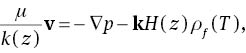

where ρf(T)=ρ0[1 – α(T – T0)],
Let us now consider the basic steady state solution of (1)–(3) as follows:
To investigate the stability of these solutions, we introduce perturbations
Then, the perturbation equations are nondimensionalized according to the scales (stars denote dimensionless quantities):
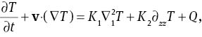
where β=(TL – TU)/d and R2 is the Rayleigh numbers. The dimensionless perturbation equations are (after omitting all stars)
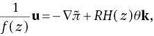

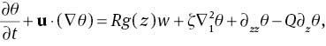
where ζ=K1/K2, u=(u,v,w) and g(z)=QeQz/(eQ – 1). These equations hold on the region {z∈(0, 1)}×{(x,y)∈ℝ2}, and the boundary conditions to be satisfied are

3 Linear and Nonlinear Energy Stability Theories
Linear instability results for stationary convection are obtained via the application of standard procedures to the linearized version of (4)–(6). The critical linear instability thresholds are located through the following eigenvalue problem for growth rate σ:


on z∈(0, 1). Here D= d/dz, w= Wei(mx+ny), θ= Θei(mx+ ny) and a2=m2 + n2 is a horizontal wave number. These equations are subject to the boundary conditions
Linearized instability theory certainly shows where instability occurs. It does not, however, a priori yield any information on stability, nor does it necessarily predict the smallest instability threshold. It is possible that nonlinear terms will make a system become unstable long before the threshold predicted by linear theory is reached. Such instabilities are called subcritical. If we have a threshold below which we know all nonlinear perturbations decay in a precise mathematical way, then this will yield a nonlinear stability boundary. When this threshold is relatively close to the analogous threshold of linear theory, we may have some confidence that the linear results are actually predicting the physical picture correctly.
The eigenvalue system of nonlinear energy stability theory for system (4)–(6) can be derive using standard approach, [27]. Let V be a period cell for a disturbance to (4)– (6), and let ||·|| and 〈·,·〉 be the norm and inner product on L2(V). We derive energy identities by multiplying (4) by u, (8) by θ and integrating on V, we obtain

where
where ϒ(z)=λH(z) + g(z) with λ a positive parameter to be chosen suitably later. We define
where H is the space of admissible functions, namely
From (12), on taking into account (13) and applying the Poincaré inequality, we find
Thus, letting γ=ϖ(RE – 1)/RE and integrating we have
If RE>1, then as t → ∞, E(t) tends to zero at least exponentially, so we have shown the decay of θ and the decay of u then clearly follows. Now, to solve the maximisation problem (13), we introduce the Euler Lagrange equations. The Euler Lagrange equations are found from
Thus, the Euler Lagrange equations which arise from the variational problem 1/RE=maxH(I/D) can be written as:

where ς is a Lagrange multiplier. To remove the Lagrange multiplier we take the third component of the double curl of (16), then, we introduce the normal mode representation, to arrive


To (19) and (20) we add the boundary conditions
4 Numerical Technique
In this section, we use the Chebyshev collocation method to solve the eigenvalue systems (9)–(10) and (19) and (20). Firstly, the systems (9)–(10) is transformed onto the Chebyshev domain (–1,1) and the solutions W and θ treated as independent variables and expanded in a series of Chebyshev polynomials
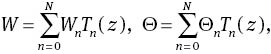
then, we insert (22) into the equations (13)–(14), and then substitute the Gauss–Labatto points which are defined by
Thus, we obtain 3N – 3 algebraic equations for 3N + 3 unknowns W0, …, WN, Θ0, …, ΘN, Φ0, …, ΦN. Now, we can add six rows using the boundary conditions (11) as follows
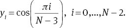
The inner product of each equation is taken with some Tk and the orthogonality of the Chebyshev polynomials exploited to obtain the following generalised eigenvalue problem:
where X=(W0, …, WN, Θ0, …, ΘN), O is the zeros matrix,
We have solved (24) for eigenvalues σj by using the QZ algorithm from Matlab routines. Once the eigenvalues σj are found we use the secant method to locate where
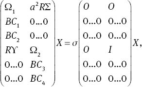
Returning to the nonlinear eigenvalue system (19) and (20), the Chebyshev collocation method yields
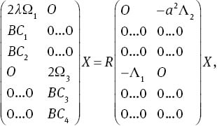
where
and
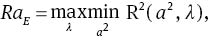
Then, we can determine the critical Rayleigh RaE for fixed a2 and λ. Next, we employ golden section search to minimise in a2 and then maximise in λ to determine RaE for nonlinear energy stability,
where for all R2<RaE we have stability. In fact, the optimization problem (26) turns out to be very tricky. Numerically, it was found that there are local maxima, and one has to be very careful when searching to locate a maximum which is useful. Numerical results are reported in the next section and compared to those of linear instability theory.
5 Stability Analysis Results
The numerical results are presented for the gravity field g(z)=1 – εz and f(z)=1 + λ1z, whereeas the numerical routine is applicable to a wide variety of other fields. To investigate the possibility of a very widely varying gravity field (one which even changes sign) we choose ε to vary from 0 to 1.
Figure 1 shows the effect of increasing ε on the critical Rayleigh number for Q= 2, λ1=0.5 and ζ=1. It is noteworthy that the nonlinear stability curves are close to those of linear theory. This shows that possible subcritical instabilities may only arise in a very small range of Rayleigh numbers, and it also demonstrates that linear instability theory is correctly capturing the physics of the onset of convection. Figure 1 demonstrates that Ra increases with increasing ε which shows the stabilizing effect of ε.
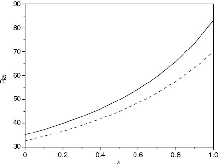
Visual representation of linear instability (solid line) and nonlinear stability (dashed line) thresholds, with critical Rayleigh number plotted against ε, where Q= 12, λ1=0.5 and ζ=1.
Figure 2 shows the effect of increasing ζ on the critical Rayleigh where Q=2, λ1=1, and ε=0.5. It is clear from this figure that Ra increases with increasing ζ which refers to the stabilizing effect of ζ. When ζ is small, it should be observed that the nonlinear Ra values are very close to the linear ones. Thus, the linear theory predicts the onset of convection accurately. However, the difference between the critical Rayleigh numbers for linear instability and nonlinear energy stability increases with increasing ζ values.
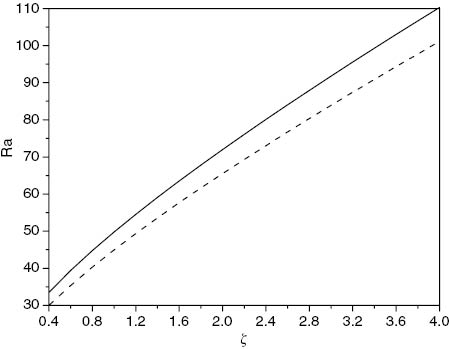
Visual representation of linear instability (solid line) and nonlinear stability (dashed line) thresholds, with critical Rayleigh number plotted against ζ, where Q= 12, λ1=0.5 and ε=0.5.
Figure 3 shows how increasing λ1 corresponds in general to greater destabilization. Again, it is very noticeable that the nonlinear energy stability curves are close to those of linear instability. This is reinforcing the fact that the linear curves are a true representation that the physics of the onset of convection is being correctly reflected. The gap between the curves represents the small band where subcritical bifurcation may possibly occur.
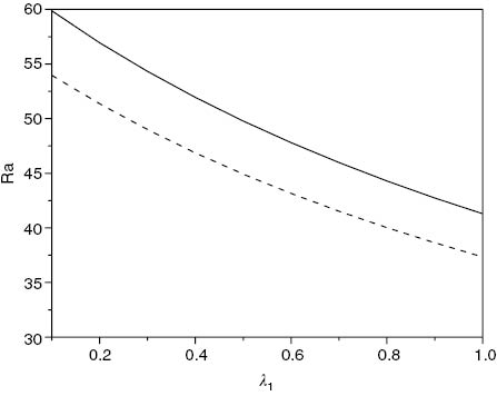
Visual representation of linear instability (solid line) and nonlinear stability (dashed line) thresholds, with critical Rayleigh number plotted against λ1, where Q=12, ζ=1 and ε=0.5.
A visual representation of the linear instability and global nonlinear stability thresholds is given in Figures 4 and 5. To assist in the interpretation of the results, we recall that ascending and descending throughflow are represented by the positivity and negativity of the value of Q, respectively. Figures 4 and 5 clearly demonstrate that the linear and unconditional nonlinear thresholds have excellent agreement for 0 ≤ Q ≤ 4. When Q is negative, the thresholds demonstrate less substantial agreement.
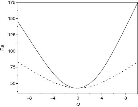
Visual representation of linear instability (solid line) and nonlinear stability (dashed line) thresholds, with critical Rayleigh number plotted against Q, where λ1=0.5, ζ=1 and ε=0.5.
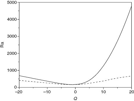
Visual representation of linear instability (solid line) and nonlinear stability (dashed line) thresholds, with critical Rayleigh number plotted against Q, where λ1=0.5, ζ=5 and ε=1.
6 Three-Dimensional Simulations
In this article, we present an efficient, stable, and accurate finite difference schemes in the vorticity-vector-potential formulation for computing the convective motion of an incompressible fluid in a porous solid. The emphasis is on three dimensions and nonstaggered grids. We introduce a second-order accurate method based on the vorticity-vector-potential formulation on the nonstaggered grid whose performance on uniform grids is comparable with the finite scheme. We pay special attention to how accurately the divergence-free conditions for vorticity, velocity, and vector potential are satisfied. We derive the three-dimensional analog of the local vorticity boundary conditions.
By using the curl operator to (4), one gets the following dimensionless form of the vorticity transport equation:
where the vorticity vector ω=(ξ1, ξ2, ξ3) is defined as

To calculate velocity from vorticity, it is convenient to introduce a vector potential ψ=(ψ1, ψ2, ψ3), which may be looked upon as the three-dimensional counterpart of two-dimensional stream function. The vector potential is defined by

It easy to show the existence of such a vector potential for a solenoidal vector field (∇·u=0). Such a vector potential can be required to be solenoidal, i.e.,

Substituting (29) in (28) and using (30) yields

The set of equations (6), (27), (29) and (31) with appropriate boundary conditions were found to be a convenient form for numerical computations. The discretised form of these equations using second-order finite difference scheme can be written as
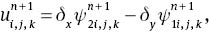
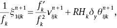
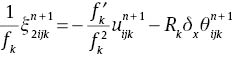

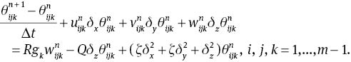
where
To solve (32)–(39) using Gauss–Seidel iteration method, in the first time level we give an initial values to the solutions. Then, we use these initial values to compute new values of solution, and the programme will continue in this process until satisfying the convergence criteria which is
where the indices k and k+ 1 refer to the solutions in iteration steps k and k+ 1, respectively. The values of the solutions in the last time level n will be the initial values to the next time level n+ 1.
Here, we should mention that our scheme is flexible for various R values and, thus, the grid resolution has been selected according to the Ra values. We decrease the values of Δx, Δy, and Δz as the value of R increases. For our problem, we find that Δx= Δy=Δz= 0.02 is enough to give us accurate results.
7 Numerical Results
In this section, RaL, is the critical Rayleigh number for linear instability theory and RaE is the critical Rayleigh number for the global nonlinear stability theory. The corresponding critical wave numbers of the linear instability and the global nonlinear stability will be denoted by aL and aE, respectively. In Table 1, we present numerical results of the linear instability and nonlinear stability analyses. The dimensions of the box, which are calculated according to the critical wave number, are shown in Table 1. We assume that the perturbation fields (u, θ, H) are periodic in the x and y directions and denoted by
Critical Rayleigh and wavenumbers
| Q | RaL | RaE | λ | ||
|---|---|---|---|---|---|
| –12 | 430.7346813 | 33.16928351 | 288.6563395 | 12.73121491 | 1.680574242 |
| 12 | 1778.657379 | 18.58281978 | 452.4411301 | 24.72135955 | 1.701997193 |
For numerical solutions of three dimensions problems, we used Δt= 5×10⁻⁵ and Δx= Δy= Δz= 0.02. The convergence criteria has been selected to make sure that the solutions arrive to a steady state. The convergence criteria are
and we select η2=10–6. The programme will continue in computing the results of the temperature, velocity, vorticity, and potential vector for new time levels until the results stratify the convergence criteria, otherwise, we stop the programme after 80,000 time levels, i.e., at the time τ=4.
In order to display the numerical results clearly, the temperature, velocity, and vorticity contours are plotted in Figures 6–9 at Ra=421 and Ra=1688. In these figures, the temperature, velocity, and vorticity contours are presented at the time level τ=4 as the possibility of arriving the solution to any steady state impossible. Figures 6–9 show the contours of u, v, w, and θ, respectively, at z=0.05, z=0.5 and z=0.95 in a, b and c for Q=– 12, λ1=0.5, ζ=5 and ε=1 and Ra=421. Also, Figures 6–9 show the contours of u, v, w, and θ, respectively, at z=0.05, z=0.5 and z=0.95 in c, d and e for Q=12, λ1=0.5, ζ=5 and ε=1 and Ra=1688.
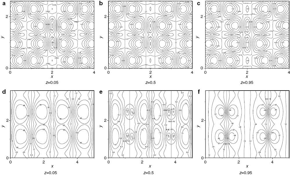
Contour plot of u for λ1=0.5, ζ=5 and ε=1. In (a), (b), (c) Q=– 12, τ=4 and Ra=421. In (d), (e), (f) Q=12, τ=1.159 and Ra=1688.
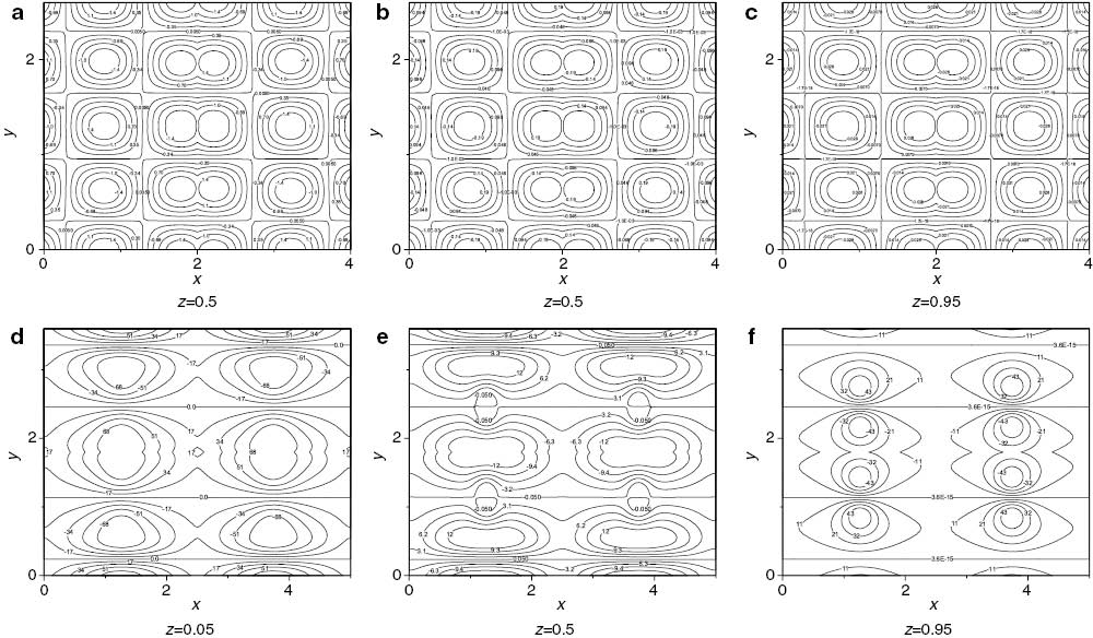
Contour plot of v for λ1=0.5, ζ=5 and ε=1. In (a), (b), (c) Q=– 12, τ=4 and Ra=421. In (d), (e), (f) Q=12, τ=1.159 and Ra=1688.
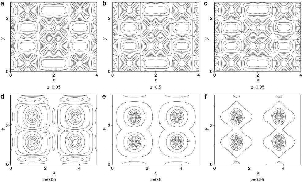
Contour plot of w for λ1=0.5, ζ=5 and ε=1. In (a), (b), (c) Q=– 12, τ=4 and Ra=421. In (d), (e), (f) Q=12, τ=1.159 and Ra=1688.
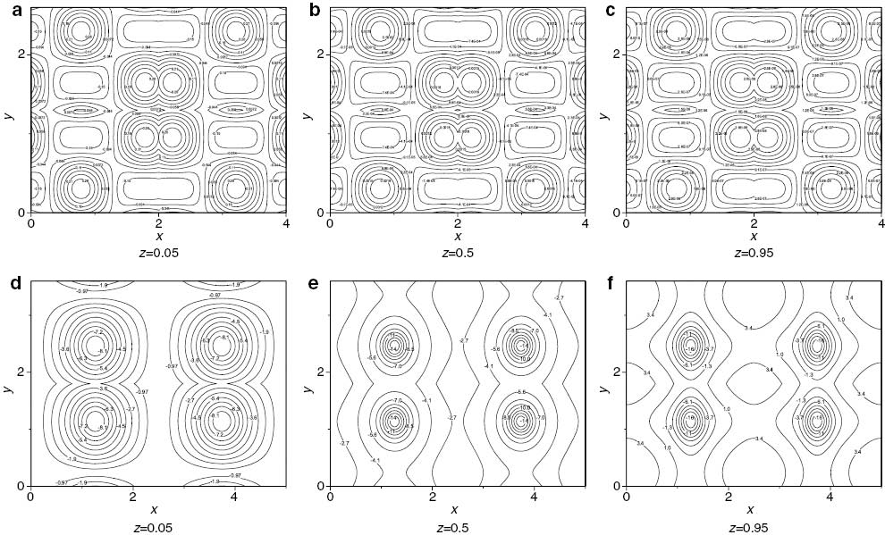
Contour plot of θ for λ1=0.5, ζ=5 and ε=1. In (a), (b), (c) Q=– 12, τ=4 and Ra=421. In (d), (e), (f) Q=12, τ=1.159 and Ra=1688.
Figures 6–9 plot the contours of u, v, w and θ respectively, at λ1=0.5, ζ=5 and ε=1 for two cases: Case1 Q=– 12, τ=4 and Ra=421, case2 Q=12, τ=1.159 and Ra=1688. Figure 6 plots the contour of perturbation velocity u for three positions z=0.05, z=0.95, and z=0.95. For negative throughflow Q=– 12, the effect of negative direction flow from permeability surface (bottom surface) is clearly in Figure 6a–c, where the flow direction inverse the buoyancy effect (the buoyancy flow is up where the negative throughflow is down), this effect represents by multi-rotating cells have lower intensity than the positive direction of throughflow (Fig. 6d–f). These cells in a, b, and c are a sequence in sign of rotating (counter clockwise CCW-positive sign and clockwise CW-negative sign), where the maximum values of intensity u at the positions z=0.05, 0.5 and 0.95 are 1.1,0.15 and 0.021, respectively. The cells in d, e, and f are more restricted and have value greater than a, b, and c, because the effect of the throughflow add to the effect of buoyancy (same direction to up). The maximum values of intensity u at Q=12 and the positions z=0.05, 0.5 and 0.95 are 66,13 and 49, respectively.
Figure 7 indicates the contours of perturbation velocity v at Q=– 12 (Fig. 7a–c) and Q=12 (Fig. 7d–f). It can be seen that the behaviour of velocity v is similar to velocity u except the cells are extended horizontally, and the sequence of the sign becomes row of cells. Also, the intensity of velocity v for Q=12 (d, e, and f) is greater than Q=– 12 a, b, and c, and the reason as mentioned in the previous section. The maximum magnitudes of v are 1.4,0.19 and 0.028 for a, b, and c, respectively, and 68, 12 and 43 for d, e, and f, respectively.
The distribution of velocity w is presented in Figure 8 for Q=– 12 (Fig. 8a–c) and Q=12 (Fig. 8d–f). This figure shows there are multiple cells for Q=– 12 and approximately four cells for Q=12. The size of cells for Q=12 (Fig. 8d–f) are reduced towards the upper plane, where the cell at z=0.95 is smallest. The magnitude of velocity w becomes maximum (wmax=58) at z=0.95 for Q=12, because the effect of density difference (TL>TU) to up and the throughflow to up (the permeability effect to up) which make the velocity maximum.
Finally, the contour of perturbation temperature θ is cleared at Figure 9 at z=0.05,0.5 and 0.95. The value of exact temperature is equal to mean temperature and perturbation temperature θ; therefore, the minus sign of θ means reduced in exact temperature. The number of cells approximately four cells for Q=12 whereas for Q=– 12 there are many cells with different signs. The value θ is reduced towards the upper surface (θ=– 8.1,– 14 and – 16 at z=0.05, 0.5 and 0.95 respectively), this is returned to boundary conditions where T=TL at z=0 and T=TU at z=d (TL>TU).
In Figures 10 and 11, we show a summary of the numerical results where we introduce the maximum and minimum values of velocities vs. time. The solid, dash, dot, dash dot, dash dot dot, and short dash lines represent umax, umin, vmax, vmin, wmax, and wmin, respectively. In Figure 10, we select Q=– 12, λ1=0.5, ζ=5, and ε=1, then according to the stability analysis, we have RaL=430.7346813 and RaE=288.6563395. Here, it clear that we have very large subcritical stability region, as there is a big difference between the critical Rayleigh numbers of linear and nonlinear theories. From Figure 10, for Ra=400, we can see that the solutions satisfy the convergence criterion at τ=0.8068 and, thus, the solution arrives to the basic steady state within a short time. However, for Ra=410, the program needs τ=1.32115, to arrive to the basic steady state, which is expected, as the required time to arrive at a steady state increases with increasing Ra values until the solution does not arrive at any steady state. Moreover, for Ra=420, the solutions do not satisfy the convergence criterion, and the program stops at τ=4, but it is very clear that the solutions can achieve the convergence criterion the next times. For Ra=421 and Ra=422, the solutions could not arrive at any steady state and the program did not progress beyond τ=4 and we let the programme run for a significant period to test the convection’s long-time behaviour. We see that the values of the velocities increase at τ=8, and then decrease at τ=12 and continue in this oscillation. For Ra=421 and Ra=422, the convection behaviour oscillated and access to a stable state was impossible. Finally, for Ra=424, the solutions arrive at a steady state early at τ=2.9461, but this steady state is completely different from the basic one. For Ra=424, here, according to the numerical results, the linear instability threshold is very close to the actual threshold, i.e., the solutions arrive to the basic steady state before the linear instability threshold.
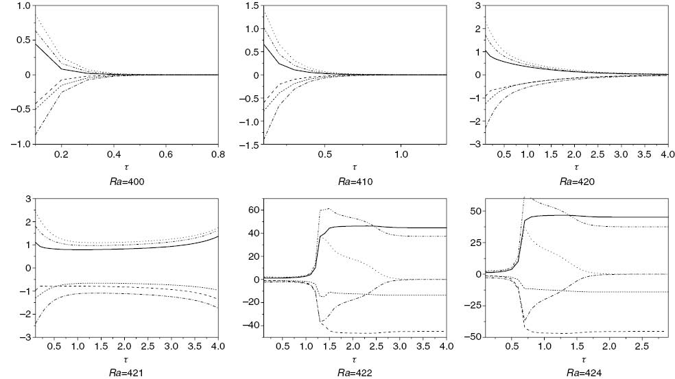
The numerical results for different Ra. We present the results for the maximum and minimum values of velocities vs. time for Q=– 12, λ1=0.5, ζ=5 and ε=1, RaL=430.7346813, RaE=288.6563395.
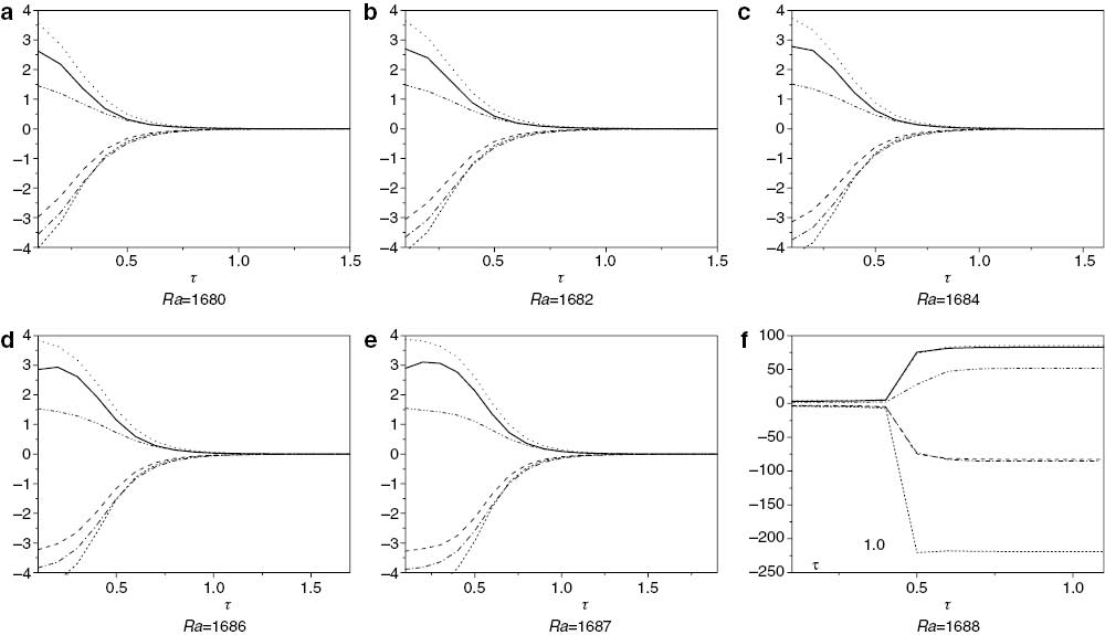
The numerical results for different Ra. We present the results for the maximum and minimum values of velocities vs. time for Q=12, λ1=0.5, ζ=5 and ε=1, RaL=1778.657379, RaE=452.4411301.
In Figure 11, critical Rayleigh numbers for Q=12, λ1=0.5, ζ=5 and ε=1 were computed, (9)–(10) and (19)–(20) were solved, leading to the following stability results: RaL=1778.657379, RaE=452.4411301. In this case, the difference between the critical Rayleigh numbers of linear and nonlinear theories is very large. Figure 11 shows that for Ra=1680, Ra=1682, Ra=1684, Ra=1686, and Ra=1887, the solutions quickly go to the basic steady state and satisfy the convergence criteria at τ=1.53815, τ=1.59605, τ=1.6704, τ=1.7892, and τ=1.93085, respectively. Moreover, for Ra=1888, the solutions arrive at a steady state and the program stops at τ=1.159. For Ra=the convection behaviour was very oscillated, and the access to the basic steady state was impossible. The results of Figure 11 explains that the stability behaviour is similar to the stability behaviour of Figure 10, as we found that the linear instability threshold is close to the actual threshold. However, when Q is negative, it is clear that the actual threshold is very close to the linear instability threshold, whereas, for positive Q the actual threshold moves slightly from linear instability threshold. This pattern of results is similar to the behaviour of throughflow in a fluid layer (see [26]).
8 Conclusions
In this article we have explored a convection in an anisotropy and symmetry in porous media with a constant throughflow. Regions of very large subcritical instabilities, i.e., where agreement between the linear instability thresholds and nonlinear stability thresholds is poor, are studied by solving for the full three-dimensional system. Numerically, we find that the convection has three different patterns. The first picture, where Ra between RaL, and RaE, is that the solutions perturbations vanish, sending the solution back to the steady state, before the linear thresholds are reached. The required time to arrive at the steady state increases as the value of Ra increases. The second picture, where Ra is close to RaL is that solutions can tend to a steady state which is different to the basic steady state v̅= (0, 0, Tf). In the third picture, where Ra is very close or Ra>RaL, the solutions do not arrive at any steady state and oscillate.
Acknowledgments
This work was supported by the Iraqi ministry of higher education and scientific research. The author would like to thank two anonymous referees for their pointed remarks that led to improvements in the original manuscript.
References
[1] B. Straughan, Mathematical Aspects of Penetrative Convection, Longman, New York 1993.Search in Google Scholar
[2] P. H. Roberts, J. Fluid Mech. 30, 33 (1967).Search in Google Scholar
[3] P. C. Matthews, J. Fluid Mech. 188, 571 (1988).Search in Google Scholar
[4] B. Straughan and D. W. Walker, Proc. R. Soc. Lond. A 452, 97 (1996).10.1098/rspa.1996.0006Search in Google Scholar
[5] A. J. Harfash, Transp. Porous Med. 101, 281 (2014).Search in Google Scholar
[6] A. J. Harfash, Transp. Porous Med. 102, 43 (2014).Search in Google Scholar
[7] A. J. Harfash, Transp. Porous Med. 103, 361 (2014).Search in Google Scholar
[8] M. C. Kim, Korean J. Chem. Eng. 30, 1207 (2013).Search in Google Scholar
[9] M. M. Rashidi, S. Abelman, and N. Freidooni Mehr, Int. J. Heat Mass Trans. 62, 515 (2013).Search in Google Scholar
[10] S. Noreen, Z. Naturforsch. A 70, 3 (2015).10.1515/zna-2014-0221Search in Google Scholar
[11] N. S. Akbar and A. W. Butt, Z. Naturforsch. A 70, 23 (2015).10.1515/zna-2014-0164Search in Google Scholar
[12] M. Sheikholeslami, R. Ellahi, M. Hassan, and S. Soleimani, Int. J. Numer. Meth. Heat Fluid Flow 24, 1906 (2014).10.1108/HFF-07-2013-0225Search in Google Scholar
[13] M. Sheikholeslami, M. G. Bandpy, R. Ellahi, and A. Zeeshan, J Magn. Magn. Mater. 369, 69 (2014).Search in Google Scholar
[14] A. Zeeshan, R. Ellahi, and M. Hassan, Eur. Phys. J. Plus 129, 261 (2014).10.1140/epjp/i2014-14261-5Search in Google Scholar
[15] R. Ellahi, A. Riaz, S. Abbasbandy. T. Hayat, and K. Vafai, Therm. Sci. J. 18, 1247 (2014).Search in Google Scholar
[16] D. A. Nield and A. Bejan, Convection in Porous Media. 4th Ed., Springer-Verlag, New York 2013.10.1007/978-1-4614-5541-7Search in Google Scholar
[17] S. Abbasbandy, T. Hayat, R. Ellahi, and S. Asghard, Z. Naturforsch. A 64, 59 (2009).10.1515/zna-2009-1-210Search in Google Scholar
[18] T. Hayat, R. Ellahi, and F. M. Mahomed, Z. Naturforsch. A 64, 531 (2009).10.1515/zna-2009-9-1001Search in Google Scholar
[19] A. J. Harfash and A. A. Hill, Int. J. Heat Mass Trans. 72, 609 (2014).Search in Google Scholar
[20] I. S. Shivakumara and A. Khalili, Transp. Porous Med. 53, 245 (2003).Search in Google Scholar
[21] I. S. Shivakumara and S. Sureshkumar, J. Geophys. Eng. 4, 104 (2007).Search in Google Scholar
[22] D. A. Nield and A. V. Kuznetsov, Transp. Porous Med. 87, 765 (2011).Search in Google Scholar
[23] A. A. Hill, S. Rionero, and B. Straughan, IMA J. App. Math. 72, 635 (2007).Search in Google Scholar
[24] F. Capone, M. Gentile, and A. A. Hill, Acta Mech. 208, 205 (2009).Search in Google Scholar
[25] A. J. Harfash, J. Non-Equilib. Thermodyn 139, 123 (2014).Search in Google Scholar
[26] A. J. Harfash, Transp. Porous Media, 106, 163 (2015).10.1007/s11242-014-0394-4Search in Google Scholar
[27] B. Straughan, The Energy Method, Stability, and Nonlinear Convection. Springer, Series in Applied Mathematical Sciences, Vol. 91, 2nd Ed. (2004).10.1007/978-0-387-21740-6Search in Google Scholar
©2015 by De Gruyter
Articles in the same Issue
- Frontmatter
- Spectrum and Green’s Function of a Many-Interval Sturm–Liouville Problem
- On a (3+1)-dimensional Boiti–Leon–Manna–Pempinelli Equation
- Inclined Magnetic Field Effect in Stratified Stagnation Point Flow Over an Inclined Cylinder
- Interaction between Barium Oxide and Barium Containing Chloride Melt
- Boundary-Layer Flow of Walters’ B Fluid with Newtonian Heating
- A Class of Boundary Value Problems Arising in Mathematical Physics: A Green’s Function Fixed-point Iteration Method
- Flow and Heat Transfer of Nanofluids Over a Rotating Porous Disk with Velocity Slip and Temperature Jump
- Soliton Solutions, Bäcklund Transformation and Lax Pair for Coupled Burgers System via Bell Polynomials
- Higher-Order Rogue Waves for a Fifth-Order Dispersive Nonlinear Schrödinger Equation in an Optical Fibre
- Solving Fractional Partial Differential Equations with Variable Coefficients by the Reconstruction of Variational Iteration Method
- A Direct Comparison between the Negative and Positive Effects of Throughflow on the Thermal Convection in an Anisotropy and Symmetry Porous Medium
- Corrigendum
- Corrigendum to: Kaluza-Klein Cosmological Model, Strange Quark Matter, and Time-Varying Lambda