Inclined Magnetic Field Effect in Stratified Stagnation Point Flow Over an Inclined Cylinder

1 Introduction

Analysis of flow past a permeable and impermeable stretching surface has gained considerable interest from researchers and scientists owing to its large number of applications in industrial and technological processes. Such flow analysis with heat transfer becomes more significant because the properties of the final product depend on two aspects: (i) the cooling liquid that is utilised and (ii) the stretching rate. Applications of such phenomenon include food-stuff processing, wire and fibre coating, chemical processing equipment, textile and paper industries, design of heat exchangers, and crystalline materials. Mukhopadhyay [1] analyzed the boundary layer flow and heat transfer over a stretching cylinder under the influence of uniform magnetic field and slip condition. Turkyilmazoglu [2] investigated the three-dimensional flow of electrically conducting viscous fluid induced by a stretching rotating disk. Bhattacharyya [3] examined the unsteady stagnation point flow caused by shrinking/stretching sheet. Rashidi et al. [4] analyzed the magnetohydrodynamic (MHD) and heat and mass transfer effects in flow over a permeable stretching sheet with radiation. Shehzad et al. [5] reported the axisymmetric flow of third-grade fluid by a radially stretching sheet.

The phenomenon of stagnation point has considerable interest due to its large number of applications in engineering and industries. Hiemenz [6] was the first to investigate the stagnation point flow of an incompressible viscous fluid. After that, Chiam [7] examined the flow analysis of Hiemenz [6] over a stretching surface for the case when free stream velocity is equal to the stretching velocity. He concluded that, in such a case, there exists no boundary layer. Bhattacharyya and Vajravelu [8] presented the boundary layer stagnation point flow over an exponentially shrinking sheet. Turkyilmazoglu and Pop [9] analyzed the stagnation point flow of Jeffrey fluid induced by a stretching/shrinking sheet. Mustafa et al. [10] reported the stagnation point flow of nanofluid past an exponentially stretching sheet. Hayat et al. [11] investigated the melting heat transfer effect on stagnation point flow of Maxwell fluid. Hsiao [12] explored the mixed convection flow of Maxwell fluid in the region of stagnation point with Newtonian heating. Furthermore, the analysis of stagnation point flow becomes more important with magnetohydrodynamic effect due to its widespread applications in engineering and industries. Some applications of MHD flow include the design of cooling systems with liquid metals and the manufacture of MHD generators, accelators, nuclear reactors, blood flow measurements, and pumps. Also, magnetohydrodynamic flow has applications in the physiological processes. Mukhopadhyay [13] analyzed the radiative MHD flow past an exponential permeable stretching sheet with slip condition. Hsiao [14] investigated the magnetohydrodynamic mixed convection flow of viscoelastic fluid past a permeable wedge. MHD entropy-generated flow over a porous disc with slip condition and variable properties was studied by Rashidi et al. [15]. The boundary layer flow of magnetohydrodynamic stagnation point flow of viscoelastic fluid over a stretching sheet with viscous dissipation was studied by Hsiao [16]. Hayat et al. [17] examined unsteady magnetohydrodynamic squeezing flow past a stretching plate. Sheikholeslami et al. [18] studied the MHD flow of nanofluid with thermophoresis and Brownian motion effects. Hsiao [19] examined the heat and mass transfer effects in mixed convection flow of viscoelastic fluid due to a stretching sheet with magnetic field and ohmic dissipation.

The phenomenon of stratification has an important role in many natural and industrial processes. Such phenomenon arises due to temperature and concentration variations or to mixing of fluids with different densities. Examples of stratification include thermal stratification of reservoirs and oceans, ground water reservoirs, heterogeneous mixtures in atmosphere, etc. It plays a key role in controlling the temperature and concentration differences between oxygen and hydrogen in the environments, which may affect the growth rate of various species as discussed by Ibrahim and Makinde [20]. Shehzad et al. [21] presented the thermally stratified flow of thixotropic fluid past a stretching sheet with thermal radiation. Srinivasacharya and Surender [22] studied the double stratified mixed convection flow of nanofluid over a vertical plate with porous medium. The magnetohydrodynamic flow of viscous fluid over an exponentially stretching sheet in thermally stratified medium was examined by Mukhopadhyay [23]. Hayat et al. [24] analyzed the stagnation point flow of an Oldroyd-B fluid with thermal stratification.

The aforementioned investigations show that no attempt has been made to study the double stratified flow over an inclined stretching cylinder and inclined magnetic field. Therefore our main objective was to explore the stagnation point flow with viscous dissipation in this direction. Combined heat and mass transfer effects were considered. Variable temperature and concentration were assumed at and away from the surface of the cylinder. Series solutions were obtained using the homotopy analysis method [25–32]. Numerical values of skin friction coefficient and Nusselt number were computed, and analysis of the physical interpretation of the involved parameters is given.

2 Mathematical Formulation

Consider the steady MHD mixed convection flow over an inclined stretching cylinder with double stratification. The flow behaviour was investigated in the region of the stagnation point. Here it is assumed that the cylinder makes an angle β₁, with the horizontal and magnetic field making an angle β₂ with the cylinder. Viscous dissipation was also analyzed in the temperature analysis. Variable temperature and concentration at the surface and away from the cylinder were assumed (Fig. 1). Using the boundary layer approximations, we have the governing equations as follows:

(1)∂(rv)∂r + ∂(ru)∂x = 0, (1)

(2)v∂u∂r + u∂u∂x = ueduedx + ν(∂2u∂r2 + 1r∂u∂r) + (βT(T − T∞) + βC(C − C∞))g Si nβ1 − σB02Si n2β2ρ(u − ue), (2)

(3)u∂T∂x + v∂T∂r = kρcp(∂2T∂r2 + 1r∂T∂r) + μρcp(∂u∂r)2, (3)

(4)u∂C∂x + v∂C∂r = D(∂2C∂r2 + 1r∂C∂r), (4)

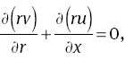
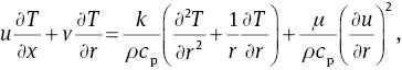
subjected to the boundary conditions

(5)u = uw = U0xl, v = 0, T = Tw(x) = T0 + a(xl), C = Cw(x) = C0 + b(xl) at r = Ru→ue = U∞xl, T = T∞ = T0 + d(xl), C = C∞ = C0 + e(xl) at r→∞. (5)

In the aforementioned expressions, u and v denote the velocity components in the axial and radial directions, respectively; U₀, U_w, and U_e are the reference, stretching and free stream velocities, respectively; g is the gravitational acceleration; β_T is the thermal expansion coefficient; β_C is the concentration expansion coefficient; T and C are the temperature and concentration of the fluid, respectively; l is the characteristic length; ν is the kinematic viscosity; ρ is the density; σ is the electrical conductivity; B₀ is the applied magnetic field; c_p is the specific heat; k is the thermal conductivity; T_w and C_w are the temperatures and concentrations at the surface, respectively; T_∞ and C_∞ are the temperatures and concentrations away from the surface, respectively; D is the mass diffusivity; a, b,d, and e are the dimensional constants; and T₀ and C₀ are the reference temperature and concentration, respectively.

Figure 1:

Physical flow model.

Using

(6)η = U0νl(r2 − R22R), ψ = UwνxRf(η)u = U0xlf′(η), v = −νU0lRrf(η), θ(η)=T − T∞Tw − T0, ϕ(η) = C − C∞Cw − C0, (6)

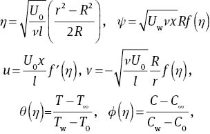
incompressibility condition is satisfied automatically and (2)–(5) are reduced to

(7)(1 + 2γη)f‴ + ff″ − (f′)2 + 2γf″ + A2+ λ(θ + Nϕ)    Si nβ1 − M2(f′ − A)Si n2β2 = 0, (7)

(8)(1 + 2γη)θ″ + 2γθ′ + Pr(fθ′ − f′θ) − Prϵ1f′    + PrEc(1 + 2γη)f″2 = 0, (8)

(9)(1 + 2γη)ϕ″ + 2γϕ′ + Sc(fϕ′ − f′ϕ − ϵ2f′) = 0 (9)

(10)f(0) = 0, f′(0) = 1, θ(0) = 1 − ϵ1, ϕ(0) = 1−ϵ2f′(∞) = A, θ(∞) = 0, ϕ(∞) = 0, (10)

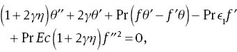
where γ is the curvature parameter, A is the ratio of the velocities, λ is the thermal buoyancy parameter, N is the ratio of concentration to thermal buoyancy, M is the Hartman number, ϵ₁ is the thermal stratified parameter, ϵ₂ is the concentration stratified parameter, Pr is the Prandtl number, Ec is the Eckert number, and Sc is the Schmidt number, which are expressed as follows:

(11)γ = (νlU0R2)1/2, λ = GrxRex2, N = Grx∗Grx, ϵ1 = da, ϵ2 = eb,Pr = μcpk,  A = U∞U0,  Sc = νD,  Ec = uw2cp(Tw − T0), M = σlρU0B0,Grx = gβT(Tw − T0)x3ν2, Grx∗ = gβC(Cw − C0)x3ν2 (11)

Skin friction, local Nusselt, and Sherwood numbers are respectively represented as follows:

(12)Cf = τwρUw2, Nux = xqwk(Tw − T0), Sh = xjwD(Cw − C0), (12)

(13)τw = μ(∂u∂r)r = R, qw = −κ(∂T∂r)r = R, jw = −D(∂C∂r)r = R. (13)

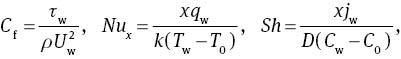
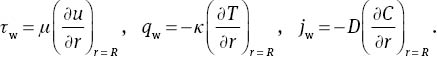
Skin friction, local Nusselt number, and Sherwood number in dimensionless forms are respectively given as

(14)CfRex1/2 = f″(0), NuxRex−1/2 = −θ′(0), ShRex−1/2 = −ϕ′(0) (14)

where Re_x=U_wl/ν.

3 Homotopic Solutions

Series solutions by homotopic technique require the initial guesses (f₀, θ₀, φ₀) and linear operators (𝓛_f, 𝓛_θ, 𝓛_φ), which are expressed in the forms

(15)f0(η) = Aη + (1 − A)(1 − exp(−η)), θ0(η)  = (1 − ϵ1)exp(−η), ϕ0(η) = (1 − ϵ2)exp(−η) (15)

(16)ℒf(f) = d3fdη3 − dfdη, ℒθ(θ) = d2θdη2−θ, ℒϕ(ϕ) = d2ϕdη2 − ϕ (16)

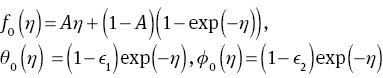
with

(17)ℒf[A1 + A2exp(η) + A3exp(−η)] = 0, (17)

(18)ℒθ[A4exp(η) + A5exp(−η)] = 0, (18)

(19)ℒϕ[A6exp(η) + A7exp(−η)] = 0, (19)

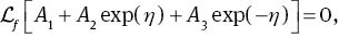
where A_i (i=1–7) are the arbitrary constants.

3.1 Convergence Analysis

Homotopy analysis technique was used for the series solutions of highly nonlinear problems, which was proposed by Liao [25]. It provides great freedom to adjust and control the convergence region of the series solutions. Therefore, we plotted the ℏ curves in Figure 2. The admissible ranges of the auxiliary parameters ℏ_f, ℏ_θ, and ℏ_ϕ are −1.25 ≤ ℏ_f ≤ −0.5, −1.3 ≤ ℏ_θ ≤ −0.6, and −1.3 ≤ ℏ_ϕ ≤ −0.6, respectively, when γ=0.2, A=0.1, λ=0.1, N=0.1, Pr=1.2, ϵ₁=0.1, ϵ₂=0.1, Sc=1.2, β₁=π/4, β₂=π/3, Ec=0.1, and M=0.1.

Figure 2:

ℏ curves for f, θ, and φ.

3.2 Discussion

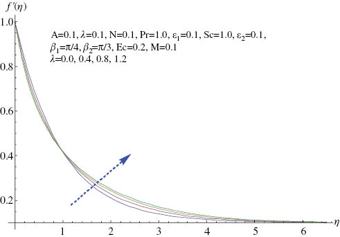
The aim of this section is to analyze the behaviour of various parameters on the velocity, temperature, and concentration distributions. The influence of A on velocity profile is presented in Figure 3. It is reported that velocity profile increases for A>1 and A<1, whereas boundary layer thickness has an opposite effect. For A=1, it was also observed that there was no boundary layer because fluid and cylinder moved with the same velocity. Figure 4. shows the variation of angle β₁ on velocity profile. It was observed that velocity and boundary layer thickness increased for larger values of angle. In fact, for higher values of angle, the buoyancy effects dominate, which increases the velocity distribution. Figure 5 shows the variation of the angle of inclination β₂ on velocity profile. It was analyzed that the velocity profile decreases for higher values of the angle. The reason for this is that, with an increase in angle, the effect of magnetic field on fluid particles increases, which consequently enhances the Lorentz force. As a result, the velocity profile decreases. It was also noted that, for β₂=0, the magnetic field has no effect on the velocity distribution, whereas maximum resistance is offered for the fluid particles when β₂=π/2. Analysis of the effect of the mixed convection parameter λ on velocity profile is shown in Figure 6. It was observed that velocity profile was higher for larger values of the mixed convection parameter because buoyancy force increases for higher values of the mixed convection parameter, which results in the enhancement of the velocity profile. Variation of the Hartman number on velocity distribution is shown in Figure 7. Velocity and boundary layer thickness decrease when the Hartman number increases. Physically, with an increase in Hartman number, the Lorentz force increases, which is a resistive force, and thus the velocity of the fluid decreases. Figure 8 shows the behaviour of the curvature parameter γ on velocity profile. It was found that velocity profile decreased near the surface of the cylinder and increased away from the surface. As the curvature parameter increases, the radius of the cylinder decreases, which results in the reduction of the cylinder area with the fluid particles. Thus the resistance offered to fluid particles decreases and, consequently, velocity profile increases. The behaviour of Eckert number Ec on temperature profile is shown in Figure 9. It was observed that temperature and thermal boundary layer thickness increase when Ec increases because more heat is generated owing to the friction caused by the increase in Ec and, as a result, the temperature profile increases. Variation of the thermally stratified parameter ϵ₁ on temperature profile is shown in Figure 10. It was noted that both temperature and thermal boundary layer thickness decrease when the thermally stratified parameter increases. The reason is that the convective flow between the heated cylinder and the ambient fluid decreases for higher values of the thermal stratification parameter; as a result, the temperature profile decreases. The behaviour of the solutal stratified parameter ϵ₂ on concentration profile is shown in Figure 11. For higher values of the solutal stratified parameter, the concentration profile decreases. It was found that the increase in ϵ₂ decreases the concentration difference between the cylinder and the ambient fluid. As a result, the concentration profile decreases.

Figure 3:

Effect of A on f′.

Figure 4:

Effect of β₁ on f′.

Figure 5:

Effect of β₂ on f′.

Figure 6:

Effect of λ on f′.

Figure 7:

Effect of M on f′.

Figure 8:

Effect of γ on f′.

Figure 9:

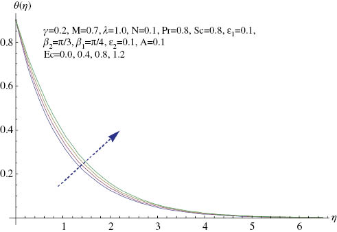
Effect of Ec on θ.

Figure 10:

Effect of ϵ₁ on θ.

Figure 11:

Effect of ϵ₂ on φ.

Table 1 shows the convergence analysis for the series solutions of governing equations. It was noted that the 26^th order of approximations is sufficient for the convergence of momentum, energy, and concentration equations. Table 2 shows the behaviour of the skin friction coefficient for various parameters. It was observed that the skin friction coefficient increases for larger values of γ, β₂, and M, whereas it decreases when A, λ, N, and β₁ are increased. Table 3 shows the effect of pertinent parameters on the Nusselt number. It was observed that the Nusselt number increases for higher values of A, λ, β₁, and M. However ϵ₁, Ec, and β₂ decrease the Nusselt number. Variations of the different parameters on the Sherwood number are shown in Table 4. Higher values of γ, λ, A, and Sc resulted in the enhancement of the Sherwood number, but it decreased with ϵ₂. Table 5 shows the comparison of f″(0) with previous existing data in the limiting case. It was observed that all the results are in good agreement with these data.

Table 1

Convergence of the series solutions for different orders of approximations when γ=0.2, A=0.1, λ=0.1, N=0.1, Pr=1.2, ϵ₁=0.1, ϵ₂=0.1, Sc=1.2, β₁=π/4, β₂=π/3, Ec=0.1, and M=0.1.

Order of approximations	−f″(0)	−θ′(0)	−ϕ′(0)
1	0.98811	1.0654	1.0911
5	1.0144	1.1440	1.1852
10	1.0168	1.1556	1.1971
15	1.0188	1.1606	1.2025
20	1.0204	1.1632	1.2053
26	1.0215	1.1645	1.2068
30	1.0215	1.1645	1.2068
35	1.0215	1.1645	1.2068

Table 2

Numerical values of the skin friction coefficient for different parameters when Pr=0.8, ϵ₁=ϵ₂=0.1, Sc=0.8, and Ec=0.2.

γ	A	λ	N	β1	β2	M	−f″(0)
0	0.1	0.2	0.1	π/4	π/3	0.3	0.9248
0.2							1.009
0.5							1.134
0.5	0						1.203
	0.2						1.052
	0.5						0.7313
	0.1	0.0					1.195
		0.2					1.134
		0.4					1.074
		0.2	0.0				1.139
			0.2				1.128
			0.5				1.112
			0.1	0.0			1.195
				π/6			1.152
				π/3			1.120
				π/4	0.0		1.084
					π/6		1.092
					π/3		1.114
					π/4	0.0	1.095
						0.3	1.134
						0.5	1.137

Table 3

Numerical values of the Nusselt number for different parameters when A=0.1, N=0.2, Sc=0.8, ϵ₂=0.2, and M=0.1.

γ	ϵ1	λ	Ec	β1	β2	Pr	−θ′(0)
0.0	0.2	0.1	0.2	π/4	π/3	0.8	0.7716
0.3							0.8737
0.5							0.9357
	0.0						1.065
	0.2						0.9357
	0.5						0.7406
	0.2	0.0					0.9293
		0.2					0.9425
		0.5					0.9622
		0.1	0.0				1.006
			0.2				0.9357
			0.5				0.8365
			0.2	0.0			0.9292
				π/4			0.9357
				π/3			0.9470
				π /4	0.0		0.9465
					π/4		0.9453
					π/3		0.9357
						0.8	0.9357
						1.0	1.027
						1.3	1.151

Table 4

Numerical values of the Nusselt number for different parameters when N=0.2, Pr=1.3, ϵ₁=0.2, β₁=β₁=π/4, Ec=0.2, and M=0.1.

γ	ϵ2	λ	A	Sc	−ϕ′(0)
0.0	0.2	0.2	0.1	0.8	0.8249
0.3					0.9384
0.5					1.011
	0.0				1.161
	0.2				1.011
	0.5				0.8754
	0.2	0.0			1.006
		0.2			1.011
		0.4			1.016
		0.2	0.0		0.9936
			0.1		1.011
			0.4		1.073
			0.1	0.8	1.011
				1.0	1.114
				1.2	1.211

Table 5

Comparison of f″(0) with those of Mahapatra and Gupta [33], Pop et al. [34] and Sharma and Singh [35] for different values of A when γ=0, λ=0, N=0, β₁=0, β₂=0, and M=0.

A	Mahapatra and Gupta [33]	Pop et al. [34]	Sharma and Singh [35]	Present results
0.1	−0.9694	−0.9694	−0.969386	−0.96939
0.2	−0.9181	−0.9181	−0.9181069	−0.91811
0.5	−0.6673	−0.6673	−0.667263	−0.66726
0.7				−0.43346
0.8				−0.29929
0.9				−0.15458
1.0				0.00000

4 Conclusion

• Velocity and temperature distributions are higher for smaller values of stratified parameters due to temperature.

• Velocity profile increases with β₁, but it decreases with β₂.

• Mixed convection parameter enhances the velocity, but it decreases the temperature distribution.

• Eckert number results in the enhancement of temperature distribution.

• Solutal stratified parameter results in the reduction of the concentration profile.

References

[1] S. Mukhopadhyay, Ain Shams Eng. J. 4, 317 (2013).Search in Google Scholar
[2] M. Turkyilmazoglu, Acta Mech. Sin. 28, 335 (2012).Search in Google Scholar
[3] K. Bhattacharyya, Ain Shams Eng. J. 4, 259 (2013).Search in Google Scholar
[4] M. M. Rashidi, B. Rostami, N. Freidoonimehr, and S. Abbasbandy, Ain Shams Eng. J. 5, 901 (2014).Search in Google Scholar
[5] S. A. Shehzad, A. Alsaedi, and T. Hayat, PLos One 8, e68139 (2013).10.1371/journal.pone.0068139Search in Google Scholar PubMed PubMed Central
[6] K. Hiemenz, Dinglers Polytechn. J. 326, 321 (1911).Search in Google Scholar
[7] T. C. Chiam, J. Phys. Soc. Jpn. 63, 2443 (1994).Search in Google Scholar
[8] K. Bhattacharyya and K. Vajravelu, Commun. Nonlinear Sci. Numer. Simul. 17, 2728 (2012).Search in Google Scholar
[9] M. Turkyilmazoglu and I. Pop, Int. J. Heat Mass Transfer 57, 82 (2013).10.1016/j.ijheatmasstransfer.2012.10.006Search in Google Scholar
[10] M. Mustafa, M. A. Farooq, T. Hayat, and A. Alsaedi, PLos One 8, e61859 (2013).10.1371/journal.pone.0061859Search in Google Scholar PubMed PubMed Central
[11] T. Hayat, M. Farooq, and A. Alsaedi, Int. J. Numer. Methods Heat Fluid Flow 24, 760 (2014).10.1108/HFF-09-2012-0219Search in Google Scholar
[12] K. L. Hsiao, Arab. J. Sci. Eng. 39, 4325 (2014).Search in Google Scholar
[13] S. Mukhopadhyay, Ain Shams Eng. J. 4, 485 (2013).Search in Google Scholar
[14] K. L. Hsiao, Int. J. Nonlinear Mech. 46, 1 (2011).10.1016/j.ijnonlinmec.2010.06.005Search in Google Scholar
[15] M. M. Rashidi, N. Kavyani, and S. Abelman, Int. J. Heat Mass Transfer 70, 892 (2014).10.1016/j.ijheatmasstransfer.2013.11.058Search in Google Scholar
[16] K. L. Hsiao, Can. J. Chem. Eng. 89, 1228 (2011).Search in Google Scholar
[17] T. Hayat, A. Qayyum, and A. Alsaedi, Eur. Phys. J. Plus 128, 157 (2013).10.1140/epjp/i2013-13157-2Search in Google Scholar
[18] M. Sheikholeslami, M. G. Bandpy, D. D. Ganji, P. Rana, and S. Soleimani, Comput. Fluids 94, 147 (2014).10.1016/j.compfluid.2014.01.036Search in Google Scholar
[19] K. L. Hsiao, Commun. Nonlinear Sci. Numer. Simul. 15, 1803 (2010).Search in Google Scholar
[20] W. Ibrahim and O. D. Makinde, Comput. Fluids. 86, 433 (2013).Search in Google Scholar
[21] S. A. Shehzad, M. Qasim, A. Alsaedi, T. Hayat, and M. S. Alhothuali, Eur. Phys. J. Plus 128, 7 (2013).10.1140/epjp/i2013-13007-3Search in Google Scholar
[22] D. Srinivasacharya and O. Surender, Appl. Nanosci. 5, 29–38 (2015).Search in Google Scholar
[23] S. Mukhopadhyay, Alexandria Eng. J. 52, 259 (2013).Search in Google Scholar
[24] T. Hayat, Z. Hussain, M. Farooq, A. Alsaedi, and M. Obaid, Int. J. Nonlinear Sci. Numer. Simul. 15, 77 (2014).Search in Google Scholar
[25] S. J. Liao, Homotopy Analysis Method in Non-linear Differential Equations, Springer and Higher Education Press, Heidelberg 2012.10.1007/978-3-642-25132-0Search in Google Scholar
[26] M. Turkyilmazoglu, Commun. Nonlinear Sci. Numer. Simul. 17, 4097 (2012).Search in Google Scholar
[27] O. A. Beg, M. M. Rashidi, T. A. Beg and M. Asadi, J. Mech. Med. Biol. 12, 1250051 (2012).Search in Google Scholar
[28] M. M. Rashidi, S. C. Rajvanshi, and M. Keimanesh, Int. J. Numer. Methods Heat Fluid Flow 22, 971 (2012).10.1108/09615531211271817Search in Google Scholar
[29] S. A. Shehzad, A. Alsaedi, and T. Hayat, Br. J. Chem. Eng. 30, 897 (2013).Search in Google Scholar
[30] S. Abbasbandy and M. Jalili, Numer. Algor. 64, 593 (2013).Search in Google Scholar
[31] T. Hayat, A. Shafiq, and A. Alsaedi, PLos One 9, e83153 (2014).10.1371/journal.pone.0083153Search in Google Scholar PubMed PubMed Central
[32] S. Abbasbandy, T. Hayat, A. Alsaedi, and M. M. Rashidi, Int. J. Numer. Methods Heat Fluid Flow 24, 390 (2014).10.1108/HFF-05-2012-0096Search in Google Scholar
[33] T. R. Mahapatra and A. Gupta, Heat Mass Transfer 38, 517 (2002).10.1007/s002310100215Search in Google Scholar
[34] S. Pop, T. Grosan, and I. Pop, Techn. Mech. 25, 100 (2004).Search in Google Scholar
[35] P. Sharma and G. Singh, J. Appl. Fluid Mech. 2, 13 (2009).Search in Google Scholar
©2015 by De Gruyter
Articles in the same Issue
- Frontmatter
- Spectrum and Green’s Function of a Many-Interval Sturm–Liouville Problem
- On a (3+1)-dimensional Boiti–Leon–Manna–Pempinelli Equation