Incorporation of phase information for improved time-dependent instrument recognition
-
Markus Schwabe
 ,
Omar Elaiashy
,
Omar Elaiashy

Abstract
Time-dependent estimation of playing instruments in music recordings is an important preprocessing for several music signal processing algorithms. In this approach, instrument recognition is realized by neural networks with a two-dimensional input of short-time Fourier transform (STFT) magnitudes and a time-frequency representation based on phase information. The modified group delay (MODGD) function and the product spectrum (PS), which is based on MODGD, are analysed as phase representations. Training and evaluation processes are executed based on the MusicNet dataset. By the incorporation of PS in the input, instrument recognition can be improved about 2% in F1-score.
Zusammenfassung
Die zeitabhängige Schätzung von in Musikaufnahmen spielenden Instrumenten ist eine wichtige Vorverarbeitung für mehrere Musikverarbeitungsalgorithmen. In diesem Ansatz wird die Instrumentenerkennung mithilfe eines neuronalen Netzes umgesetzt, das einen zweidimensionalen Eingang aus Beträgen der Kurzzeit-Fourier-Transformation (STFT) und einer auf Phaseninformation basierender Zeit-Frequenz-Darstellung besitzt. Die modifizierte Gruppenlaufzeit (MODGD) und das Produktspektrum (PS), welches auf der MODGD basiert, werden als Phasendarstellungen analysiert. Trainings- und Evaluationsprozess werden auf Basis des MusicNet-Datensatzes durchgeführt. Durch die Einbeziehung des PS im Eingang kann die Instrumentenerkennung um etwa 2% im F1-Score verbessert werden.
1 Introduction
Instrument recognition is highly relevant for different tasks in music signal processing. For music information retrieval (MIR), the playing instruments in polyphonic music signals are important features that are used as a part of the audio tags in automatic tagging [3]. Additionally, the information about playing instruments can facilitate the detection of other instrument-dependent features and tags like genre or mood. Furthermore, audio source separation and automatic music transcription, as for example in [10], can be improved by instrument recognition in preprocessing, because the separation or transcription algorithm shrinks to a tailored estimation for a much smaller amount of known instruments.
Most of instrument recognition algorithms have focused on clip-wise recognition, which means that the playing instruments were estimated for the whole music excerpt fed to the algorithm. Han et al. [5] developed a deep convolutional neural network (CNN) for instrument recognition based on mel-spectrogram inputs and aggregation of multiple outputs from sliding windows over the audio data. Pons et al. [9] analyzed the architecture of CNNs in order to formulate an efficient design strategy to capture the relevant information about timbre. Both approaches were trained and validated by the IRMAS dataset [2] of polyphonic music excerpts.
In order to consider not only the absolute values of the audio data, like it is done through the transformation of mel-spectograms, Li et al. [8] built a CNN for raw music signals as input data. This network, as the CNN for automatic tagging of Dieleman and Schrauwen [3], is a so-called end-to-end learning approach and needs only very little domain knowledge. But compared to approaches with preprocessed input data such as spectrograms, end-to-end learning performs slightly lower [5]. Another possibility for the incorporation of the whole signal information is the usage of phase information derived from a signal transform, for example the Fourier transform. Combined with MFCCs, Diment et al. [4] used the modified group delay (MODGD) feature, including phase information calculated from the Fourier transform, to train Gaussian mixture models for instrument recognition. Sebastian and Murthy [11] trained a recurrent neural network for music source separation with a phase representation of music signals derived from the MODGD features.
Especially for improving audio source separation by preprocessed instrument recognition, the clip-wise recognition is not sufficient. Thus, frame-level instrument recognition was developed by Hung and Yang [6]. They used the absolute values of the constant-Q transform (CQT) and separately estimated pitch information of the music signal as input for their deep neural network. A combined estimation of the playing instruments and notes for each frame was presented by Hung et al. [7], in which the proposed model is forced to estimate the interaction between timbre and pitch.
In phase information of music signals, timbre details, for example about specific instruments, are included. Consequently, we want to improve time-dependent instrument recognition by the incorporation of phase information. As frame-level instrument recognition is too fast for the temporal resolution of the human ear, time-dependent recognition with a resolution of 100 ms is sufficient. First, the phase representations that contain the phase information are defined in Section 2. The proposed model for instrument recognition is explained in Section 3 and the experiments for the evaluation of the model are described in Section 4. In Section 5, the results are summarized.
2 Phase representations
Many MIR algorithms only use the absolute values |X[m, k]| of the short-time Fourier transform (STFT)
that is calculated from the discrete music signal x[n] and the time and frequency shifted window
The resulting phase ambiguity caused by unwrapping can be avoided by calculating the discrete realization of the continuous group delay function [1]
which is defined as [4]
where Y [m, k] is the STFT of the signal y[n] = n·x[n] and the indices R and I stand for the real and the imaginary part.
Close to zeros of the system transfer function near the unit circle in the z-domain, the absolute values of X[m, k] and therefore the denominator term of equation (3) are very small. Consequently, those zeros cause high peaks in the corresponding group delay function that superpose the relevant phase information. Windowing in the short-time analysis, like in the calculation of the STFT, induces such unwanted zeros [11]. Therefore, the signal’s STFT X[m, k] in the denominator is replaced by its cepstrally smoothed version S[m, k] in the modified group delay (MODGD) function. This function suppresses zeros of the transfer function and is defined as [4]
with
where α and γ are design parameters for the dynamic range of the MODGD function.
A combination of magnitude and phase information is realized by the product of squared absolute and group delay function values [13]
The resulting phase-dependent time-frequency representation Q[m, k] is called product spectrum (PS) in this paper.
3 Proposed model
The estimation of active instruments in the input music signal is realized by a convolutional neural network with 16 convolution layers. Its structure is described in detail in Section 3.2. In order to incorporate phase information, the network is fed on a combination of two time-frequency representations calculated in a preprocessing step before the instrument estimation, which is explained in Section 3.1. For the network’s training, the utilized dataset and the label generation are decribed in Section 3.3.
3.1 Preprocessing
Beside the common input of a time-frequency representation of magnitudes, an additional time-frequency representation based on phase information is calculated and concatenated as network input in order to improve identification of instruments in polyphonic music at frame level. In this case, the magnitude representation contains the absolute values of the STFT (Equation 1) of the analyzed music signal. As phase information representation, the MODGD feature map, calculated by Equations 4 and 5, or the product spectrum of Equation 7 is utilized.
Before time-frequency calculation, the raw audio input signal is normalized to its maximum amplitude and then divided into 3 s segments because of memory restrictions during training and operation of the neural network. Magnitude and phase representations are calculated for each segment. In the STFT calculation, a window length of 1024 samples is used, which represents 23 ms at the sampling rate of 44.1 kHz, because the input music signal is assumed to be stationary during that period. Furthermore, 50% overlap between successive windows is realized. The adjustment parameters γ and α of MODGD function are empirically selected by means of a variation over all music pieces of the dataset and their respective impact on MODGD dynamics and noise behavior. For the investigated range from 0.1 to 1, the values γ = 0.99 and α = 0.4 were the most suitable.
The resulting magnitude and phase representation values for each frequency and time bin are converted into a logarithmic scale according to
with ϵ = 10−3. This allows the consideration of high dynamics and provides a differentiated representation of the harmonics. In addition, the logarithmic representation corresponds more to human perception. Both magnitude and phase input representation are concatenated along channel dimension to cover the correlation between them in time and frequency. Consequently, the complementing representations constitute the 3-dimensional input data of shape X ∈ ℝ513×259×2.
3.2 Model architecture
Active instruments, which are present during the respective input segments, are estimated by a neural network of 16 convolution layers. Its architecture and most important layer parameters are presented in figure 1. The first 10 layers containing 2D convolution are grouped in four convolutional blocks with increasing feature kernel size from 3 to 9 in time dimension, because deeper features should comprise a wider time interval. Each convolutional block consists of more than one convolutional sub-block with 2D convolution, batch normalization for regularization and a rectified linear unit (ReLU) as activation function, colored in blue. It is followed by max pooling, colored in yellow, to reduce the dimension of feature maps in deeper layers. Furthermore, the number of kernels is increasing from 16 to 128 for each convolutional block in order to extract a large number of features with high degree of abstraction. The last 2D convolution layer, colored in blue, extracts with 2048 the largest number of features and ensures that the output shape (1, 30) for frequency and time is met. This shape realizes a time resolution of 100 ms in the instrument estimation output frames.
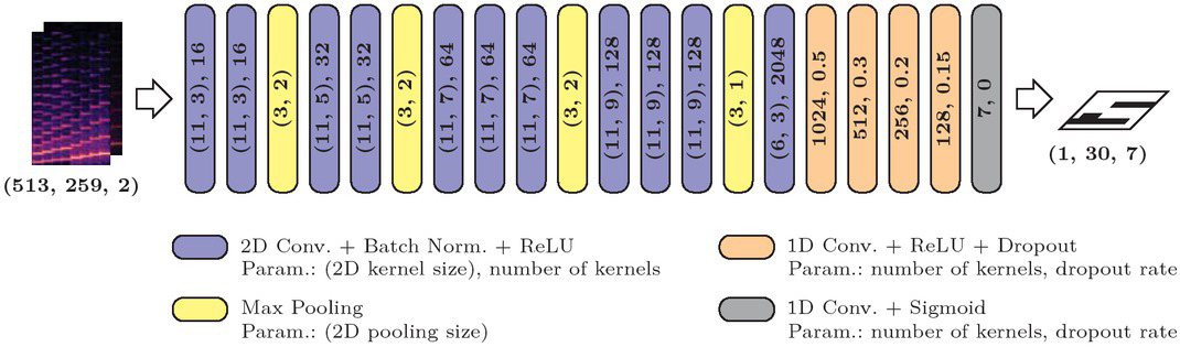
Schematic model structure with layer parameters.
The last 5 layers of the neural network are fully connected layers (FCL), which are implemented by 1×1 convolutions. Thereby, the number of kernels is interpreted as the number of nodes in a FCL. For the first four FCLs, colored in orange, dropout with the given percentage is used to improve regularization. The 7 output nodes, representing the 7 output instruments considered in the dataset (Section 3.3), are achieved by decreasing number of kernels from 1024 to 7 across the FCLs. As in the 2D convolution sub-blocks, ReLU is used as activation function, except for the output layer, colored in gray, whose activation function is the sigmoid function.
3.3 Dataset and label generation
The MusicNet dataset [12] with 34 hours of chamber music performances is utilised for training and evaluating the developed model. Thereby, the predefined partition of the 330 freely-licensed music recordings in training and test set has been used. Although there are 11 instruments in the entire dataset, only 7 instruments are active in the 10 test recordings. Consequently, only these 7 instruments piano, violin, viola, cello, clarinet, bassoon, and horn are estimated and evaluated in this work, similar to [6]. Sounds of the other 4 instruments oboe, flute, harpsichord, and string bass are not removed from training dataset, but have not been labeled. They are assumed as unwanted additional signals during training.
In order to achieve a time-dependent instrument recognition, the resolution of output time frames is chosen to be 100 ms. Thus, the model estimates the presence of instruments for 30 time frames in each 3 s segment. The corresponding label matrix of a 3 s segment, which represents the ground truth for the instrument recognition, is generated as a Boolean matrix of shape (30, 7). If an instrument has been played at any time during the particular 100 ms of a time frame, it is assumed as active and labelled with ‘1’ in the respective row for that instrument and the column for this time frame.
4 Experiments
The model described in Section 3 is trained and evaluated with the MusicNet dataset, whose labels are built according to Section 3.3. Keras with Tensorflow has been used for the model’s implementation and its application during the experiments. Further details about the implementation, especially for estimation and evaluation, are described in Section 4.1. In Section 4.2, the results of the experiments are presented and discussed.
4.1 Implementation details
Three models, mainly different concerning the input, are trained and analysed in this work. All models consider the magnitudes of the STFT as input, but one model incorporates the MODGD feature map and one model incorporates the product spectrum in a second input dimension. They are trained using stochastic gradient descend (SGD) with momentum 0.9 as the optimization algorithm. Thereby, an initial learning rate of 0.01 is defined. In order to optimize the model parameters, binary cross entropy (BCE) is used as the cost function.
Due to the sigmoid activation function in the output layer, all estimations for active instruments are continuous values in the range [0, 1], which represent probabilities for their presence at the respective time frames. Since we consider an instrument either active or not in a defined time frame, the output is binarized with a threshold b. During the evaluation, a threshold of b = 0.5 is used in most cases. Additionally, a threshold variation in steps of 0.05within [0.3, 0.7] has been analysed.
Instrument recognition results are evaluated based on the MusicNet test dataset and the F1-score. This metric is the harmonic mean of the metrics precision and recall, which are ratios of the number of right positive estimations to all positive estimations (precision) or all positive labels (recall). The F1-scores are calculated independently for each instrument, but combined for all considered test recordings. An average F1-score is calculated over all instruments and for the whole test dataset to get a simple performance metric.
4.2 Results
After the successful training, the performance of the different models is compared based on the F1-scores for the MusicNet test dataset. They are calculated as described in Section 4.1 for each instrument and an average value and are given in Table 1.
Resulting F1-scores for the MusicNet test dataset.
| Method | Piano | Violin | Viola | Cello | Clarinet | Bassoon | Horn | Average |
|---|---|---|---|---|---|---|---|---|
| STFT | 0.9812 | 0.9390 | 0.8140 | 0.8875 | 0.8442 | 0.7648 | 0.6283 | 0.8370 |
| STFT with MODGD | 0.9821 | 0.8958 | 0.7886 | 0.8344 | 0.7267 | 0.6808 | 0.4342 | 0.7632 |
| STFT with PS | 0.9814 | 0.9514 | 0.8291 | 0.9091 | 0.8720 | 0.7857 | 0.6763 | 0.8578 |
As presented in Table 1, the incorporation of the MODGD feature map doesn’t lead to an improved instrument recognition, it even leads to a worse result than the recognition with only the absolute STFT values. In contrast, the estimation of active instruments can be improved by the incorporation of the product spectrum (PS), because both the average F1-score and the F1-scores for each instrument are increased by this additional time-frequency representation in the input. This could be explained by the masking of the MODGD feature map with the STFT magnitudes in the calculation of the PS. Consequently, additional signal portions in the STFT or MODGD spectrums beside the harmonics are attenuated, if they only occur in one representation.
Further improvements can be achieved by a modified threshold b for binarization. Therefore, the influence of a threshold variation in steps of 0.05 within [0.3, 0.7] is investigated for STFT with PS input. In Table 2, the resulting F1-scores are summarized and the highest value for each instrument is highlighted. Threshold values outside the range [0.3, 0.7] are considered as too critical for binarization, because the risk of false active estimations (in case of low thresholds) or the risk of false inactive estimations (in case of high thresholds) becomes higher.
F1-scores for threshold variation with STFT and PS model.
| Threshold | Piano | Violin | Viola | Cello | Clarinet | Bassoon | Horn | Average |
|---|---|---|---|---|---|---|---|---|
| 0.3 | 0.9823 | 0.9537 | 0.8186 | 0.8890 | 0.8727 | 0.7814 | 0.6503 | 0.8498 |
| 0.35 | 0.9820 | 0.9532 | 0.8207 | 0.8951 | 0.8741 | 0.7858 | 0.6601 | 0.8530 |
| 0.4 | 0.9821 | 0.9523 | 0.8234 | 0.9006 | 0.8750 | 0.7858 | 0.6675 | 0.8552 |
| 0.45 | 0.9821 | 0.9523 | 0.8271 | 0.9045 | 0.8737 | 0.7866 | 0.6737 | 0.8571 |
| 0.5 | 0.9814 | 0.9514 | 0.8291 | 0.9091 | 0.8720 | 0.7857 | 0.6763 | 0.8578 |
| 0.55 | 0.9816 | 0.9491 | 0.8319 | 0.9108 | 0.8707 | 0.7828 | 0.6786 | 0.8579 |
| 0.6 | 0.9811 | 0.9478 | 0.8336 | 0.9093 | 0.8645 | 0.7798 | 0.6792 | 0.8565 |
| 0.65 | 0.9808 | 0.9451 | 0.8348 | 0.9093 | 0.8566 | 0.7732 | 0.6720 | 0.8531 |
| 0.7 | 0.9796 | 0.9409 | 0.8310 | 0.9076 | 0.8480 | 0.7646 | 0.6492 | 0.8458 |
The threshold with the best F1-score depends strongly on the instrument, because the number of recodings for each instrument is very unequal in the MusicNet dataset. Piano and violin are the two instruments with the most recordings in MusicNet, so their best threshold is the lowest investigated threshold. In addition, the test recordings contain solo recordings of piano, violin, and cello, but only recordings of trios for the rest of the considered instruments. As instrument recognition is much easier for solo recordings, the three solo instruments have the best F1-scores for the MusicNet test dataset. Based on the thresholds investigated, the best possible average F1-score would be the average of the highlighted values of Table 2. This best F1-score of 0.8603 can be reached by instrument dependent thresholds.
In order to evaluate the developed frame-wise instrument recognition, results for the approach of Hung and Yang [6], which is the best approach for frame-level instrument recognition in literature, are compared to our STFT with PS model in Table 3. That approach uses the CQT of the analysed music as input and additionally harmonic series features (HSF) for pitch estimation, whereas STFT is used in our approach and no pitch estimation is needed. F1-score, precision, and recall values are recalculated for the algorithm of Hung and Yang in Table 3 to utilize the same labeling strategy for all approaches. The F1-scores of the HSF-5 model are a little bit higher than those of the STFT with PS models, consequently it performs slightly better for the MusicNet test dataset. But the thresholds of the HSF-5 model are instrument-dependent and in the range [0.01, 0.99], so the instrument recognition is more robust in case of the STFT models with thresholds in the range [0.3, 0.7]. Furthermore, those different thresholds of HSF-5 are one reason for the higher precisions, but also for the lower recalls compared to our STFT with PS models. As higher recalls ensure a larger coverage of positive labels, the STFT with PS models realize an increased detection of active instruments. That is an advantage for subsequent signal processing, because the instrument detection should include most of the occurring instruments in the analysed music recording.
Evaluation metrics for instrument recognition model with harmonic series feature (HSF) [6] and the developed STFT and PS model with constant threshold b = 0.5 and best instrument dependent thresholds.
| Method | Metric | Piano | Violin | Viola | Cello | Clarinet | Bassoon | Horn | Average |
|---|---|---|---|---|---|---|---|---|---|
| HSF-5 [6] | Precision | 0.9777 | 0.9383 | 0.7678 | 0.9175 | 0.8801 | 0.7931 | 0.7061 | 0.8544 |
| Recall | 0.9904 | 0.9679 | 0.8953 | 0.9069 | 0.9237 | 0.8544 | 0.8188 | 0.9082 | |
| F1-score | 0.9840 | 0.9529 | 0.8267 | 0.9122 | 0.9014 | 0.8226 | 0.7583 | 0.8797 | |
| STFT with PS thr.: b = 0.5 | Precision | 0.9743 | 0.9382 | 0.7186 | 0.8520 | 0.8040 | 0.6875 | 0.5921 | 0.7952 |
| Recall | 0.9886 | 0.9649 | 0.9798 | 0.9743 | 0.9525 | 0.9168 | 0.7884 | 0.9379 | |
| F1-score | 0.9814 | 0.9514 | 0.8291 | 0.9091 | 0.8720 | 0.7857 | 0.6763 | 0.8578 | |
| STFT with PS best thresholds | Precision | 0.9700 | 0.9298 | 0.7395 | 0.8628 | 0.7961 | 0.6798 | 0.6616 | 0.8057 |
| Recall | 0.9949 | 0.9788 | 0.9583 | 0.9643 | 0.9711 | 0.9332 | 0.6977 | 0.9283 | |
| F1-score | 0.9823 | 0.9537 | 0.8348 | 0.9108 | 0.8750 | 0.7866 | 0.6792 | 0.8603 |
5 Conclusion
An improved frame-level instrument recognition by a neural network with STFT and phase representation as input has been proposed in this work. The modified group delay (MODGD) function has been utilized for the generation of the time-frequency representations containing the phase information. During the work, MODGD feature map and product spectrum (PS) have been investigated as additional phase representations, but only the PS achieved an improved performance compared to the simple STFT magnitude. This approach performs comparably to other frame-level approaches in the literature.
In future works, a different model architecture such as residual structure could be investigated. Furthermore, the algorithm has to be tested with larger datasets and more instruments to improve applicability in music signal processing and specific MIR tasks.
References
[1] H. Banno, J. Lu, S. Nakamura, K. Shikano, and H. Kawahara. Efficient representation of short-time phase based on group delay. In IEEE International Conference on Acoustics, Speech, and Signal Processing (ICASSP), volume 2, pages 841–864, 1998.10.1109/ICASSP.1998.675401Search in Google Scholar
[2] J. J. Bosch, J. Janer, F. Fuhrmann, and P. Herrera. A comparison of sound segregation techniques for predominant instrument recognition in musical audio signals. In 13th International Society for Music Information Retrieval (ISMIR) Conf., pages 559–564, 2012.Search in Google Scholar
[3] S. Dieleman and B. Schrauwen. End-to-end learning for music audio. In IEEE International Conference on Acoustics, Speech, and Signal Processing (ICASSP), pages 6964–6968, 2014.10.1109/ICASSP.2014.6854950Search in Google Scholar
[4] A. Diment, P. Rajan, T. Heittola, and T. Virtanen. Modified group delay feature for musical instrument recognition. In Proceedings of the 10th International Symposium on Computer Music Multidisciplinary Research, pages 431–438, 2013.Search in Google Scholar
[5] Y. Han, J. Kim, and K. Lee. Deep convolutional neural networks for predominant instrument recognition in polyphonic music. IEEE/ACM Transactions on Audio, Speech, and Language Processing, 25(1):208–221, 2017.10.1109/TASLP.2016.2632307Search in Google Scholar
[6] Y.-N. Hung and Y.-H. Yang. Frame-level instrument recognition by timbre and pitch. In 19th International Society for Music Information Retrieval (ISMIR) Conference, pages 135–142, 2018.Search in Google Scholar
[7] Y.-N. Hung, Y.-A. Chen, and Y.-H. Yang. Multitask learning for frame-level instrument recognition. In IEEE International Conference on Acoustics, Speech, and Signal Processing (ICASSP), pages 381–385, 2019.10.1109/ICASSP.2019.8683426Search in Google Scholar
[8] P. Li, J. Qian, and T. Wang. Automatic instrument recognition in polyphonic music using convolutional neural networks. arXiv preprint arXiv:1511.05520, 2015.Search in Google Scholar
[9] J. Pons, O. Slizovskaia, R. Gong, E. Gómez, and X. Serra. Timbre analysis of music audio signals with convolutional neural networks. In 25th European Signal Processing Conf., pages 2744–2748, 2017.10.23919/EUSIPCO.2017.8081710Search in Google Scholar
[10] M. Schwabe, M. Weber, and F. Puente León. Notenseparation in polyphonen Musiksignalen durch einen Matching-Pursuit-Algorithmus. 85(S1):103–109, 2018.10.1515/teme-2018-0039Search in Google Scholar
[11] J. Sebastian and H. A. Murthy. Group delay based music source separation using deep recurrent neural networks. In International Conference on Signal Processing and Communications, pages 1–5, 2016.10.1109/SPCOM.2016.7746672Search in Google Scholar
[12] J. Thickstun, Z. Harchaoui, and S. M. Kakade. Learning features of music from scratch. In International Conference on Learning Representations, 2017.Search in Google Scholar
[13] D. Zhu and K. K. Paliwal. Product of power spectrum and group delay function for speech recognition. In IEEE International Conference on Acoustics, Speech, and Signal Processing (ICASSP), volume 1, pages I125–I128, 2004.10.1109/ICASSP.2004.1325938Search in Google Scholar
© 2020 Walter de Gruyter GmbH, Berlin/Boston
Articles in the same Issue
- Frontmatter
- Editorial
- XXXIV. Messtechnisches Symposium
- Beiträge
- Detektion der Auflagestege von Flachbett-Laserschneidmaschinen mittels Nahinfrarot-Beleuchtung
- Lichtfeld-Tiefenschätzung für die Vermessung teilspiegelnder Oberflächen
- Ganzheitliche Kalibrierung von Gewinden auf Basis eines dreidimensionalen Ansatzes
- Analyse von 3D-CT-Aufnahmen von Spänen zur Extrahierung der Segmentspanbildungsfrequenz
- Resolution enhancement through nearfield-assistance in interference microscopy
- Fertigung polymerer optischer Phasenplatten zur Erzeugung von Ringmoden mittels direkter Laserlithografie
- Direct-imaging DOEs for high-NA multi-spot confocal microscopy
- Methoden zur Minimierung des Rauscheinflusses durch Hitzeflimmern bei einem heterodynen Laser-Doppler-Vibrometer
- Inverse piezoelectric material parameter characterization using a single disc-shaped specimen
- Klassifikation von Grübchenschäden an Zahnrädern mittels Vibrationsmessungen
- Incorporation of phase information for improved time-dependent instrument recognition
- Akustische Zeitumkehrfokussierung in Wasser mittels FPGA-basierter Plattform
- De-Embedding-Ansatz zur Messung nichtidealer Kapazitäten mit kommerziellen Kapazitätssensoren
- Low-cost Indirect Measurement Methods for Self-x Integrated Sensory Electronics for Industry 4.0
- Reconfigurable Wide Input Range, Fully-Differential Indirect Current-Feedback Instrumentation Amplifier with Digital Offset Calibration for Self-X Measurement Systems
- A Compact Four Transistor CMOS-Design of a Floating Memristor for Adaptive Spiking Neural Networks and Corresponding Self-X Sensor Electronics to Industry 4.0
- Monte-Carlo-Methode zur Verringerung von Messfehlern bei der Materialparameterbestimmung mit Hohlraumresonatoren
- Bestimmung des Anregungsspektrums für kontaktlose breitbandige Messungen der Übertragungsfunktion mit Plasmaanregung und Laser-Doppler-Vibrometrie
- Self-sufficient vibration sensor for high voltage lines
- Flexibler organischer elektrochemischer Transistor als Biosensor für Organ-on-a-Chip
- Erkennung und Kompensation von Vergiftung durch Siloxane auf Halbleitergassensoren im temperaturzyklischen Betrieb