
Synthesis design using mass related metrics, environmental metrics, and health metrics
-
Marco Eissen


Abstract
The efforts to integrate environmental aspects, health aspects as well as safety aspects into chemical production has led to the development of measurable and thus objectifying metrics. The application of these metrics is considered to be most promising, especially during the earliest phases of synthesis design. However, the operability in daily work suffers from the lack of available data, or a large variety of data, and the complexity of data processing. If a life cycle assessment is not practical in the early development phase, environmental factor and process mass intensity can give a quick and reliable overview. I will show that this often says the same in advance as a subsequently prepared life cycle assessment. Readers will realise that, based on preparative descriptions, they can quickly determine these metrics for individual syntheses or extensive synthesis sequences applying the available software support. Environmental relevance in terms of persistence, bioaccumulation and toxicity (PBT) can be presented using a modification of the European ranking method ‘DART’ (Decision Analysis by Ranking Techniques). Based on corresponding PBT data, readers can determine a hazard score between 0 and 1 for any substance using the spreadsheet file provided, with which the mass of (potentially emitted) substances can be weighted. Occupational health can be represented using a modification of the recognized ‘Stoffenmanager’. Both concepts are presented and spreadsheet files are offered. This article is based on a presentation which was given at the Green Chemistry Postgraduate Summer School in Venice, 6th–10th July 2020.
Introduction
The research community is united by the goal of sustainability. The journals are full of articles on better catalysts, shorter reaction paths, greener [1] solvents, less problematic substances, and more. But is one’s own research result really better or greener than what already exists? The claim is quickly made. The question [2] as to how one can be sure is justified, and the demand [3] for measurable proof is obvious. Of course, a balance provides a measurable mass indication of the manufactured product, which is yet again identified with measurable substance-specific boiling and melting temperatures, chromatography, infrared, NMR spectroscopy, mass spectrometry, and so on. However, measuring sustainability is not that simple. This is due to the fact that the three dimensions of ecology, economy and social [4] issues can be broken down into a wide variety of sub-areas. The social aspect can mean, for example, protection against hazardous chemicals for employees and residents in the vicinity of a production plant either of one’s own company or, on the other hand, a supplier in a low-wage country with possibly lower safety and environmental standards [5], and potential child labor. Further aspects could be listed. The same applies to ecological consequences. Global warming potential, acidification potential, ozone depletion potential etc. can be taken into account as well. With regard to renewable resources, land use and availability of resources are two important categories. While the first is a sensitive issue regarding concurrence with food production, the other stresses the long-term prominence towards fossil resources. These impact categories are needed for a life cycle assessment [6] according to the ISO 14044. Most impact categories have to be considered separately and could then, if desired, be aggregated according to an appropriate conversion key. The ecoinvent database [7] delivers relevant information about the ‘rucksacks’ of substances such as lime or toluene. However, the database is limited, which is why the time demand for a full life cycle assessment is normally high. The need for simplification has led to industrial tools such as the eco-efficiency method (BASF [8]) or the fast life cycle assessment (LCA) of synthetic chemistry (FLASC [9] at GSK). Also, in academic research simplified LCAs [10], [11], [12], [13], [14] are conducted. Another approach is the consideration of only the cumulative energy demand (CED), because correlations to other impact categories indicate that it could be a predictor [15] for the environmental burden. Energy-related impacts [16] often represent more than half and sometimes up to 80 % of the total impacts. However, in early synthesis design little energy data exist and high uncertainties are associated with the estimation of data concerning potential technological solutions. Interestingly, a tool is available for general use which is able to predict the CED for (petro)chemicals [17], see Fig. 1. An example molecule would be 2-chloropropane (Fig. 2).

Software EstiMol for use on the internet page of ifu hamburg, https://www.ifu.com/en/umberto/estimol/.
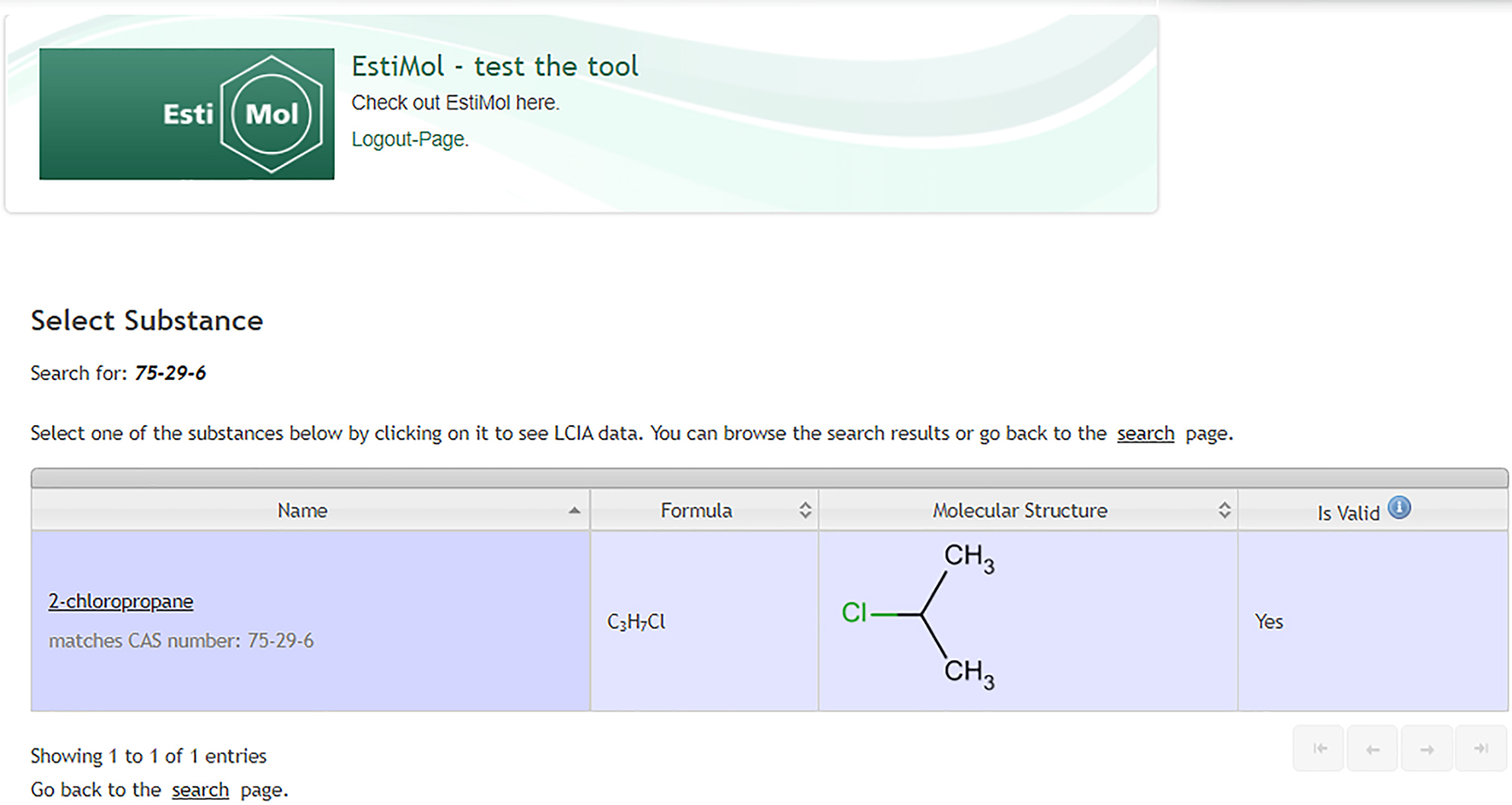
Selection of a substance for a data search.
The calculations are valid if they are in the range of 0.5–9 kg CO2-eq/kg (GWP) and from 30 to 1400 MJ-eq/kg (CED) (Fig. 2). In this case, the approximation is about 2.6 for the GWP and 69 for the CED, and the Ecoindicator 99 shows about 0.25 points (Fig. 3). Of course, these are not absolute values, but they are within a statistical range for which a standard deviation is also given.
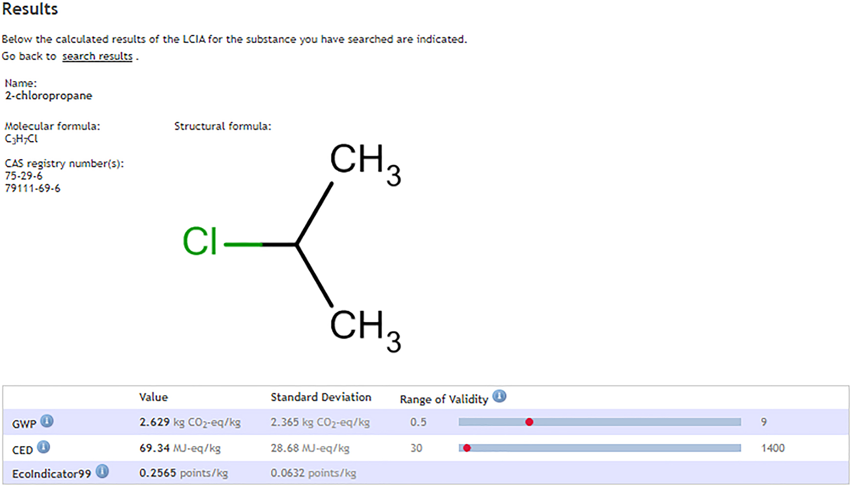
Results from the estimation for GWP, CED and Ecoindicator 99.
The methods of the different standardized procedures of a cradle-to-grave life cycle assessment differ in their approach and focus – examples are: CML – method, UBA – assessment method, Eco – Indicator 99, Sustainable Process Index (SPI), etc. A complete LCA creates degrees of freedom [18] and might open up the view for renewable raw materials [19], where refinement could produce products that are readily biodegradable. For example, pharmaceutical drugs. After they have taken effect in the body, they are released into the environment via wastewater and may have a greater environmental impact than chemical substances released during production. In this respect, a molecular design [20] with regard to rapid degradability could be purposeful and should also be taken into account in didactic [21] concepts. The overall view in a LCA allows the design of the product and the production chain to be better adapted [18] to the purpose. However, the holistic approach of a life cycle assessment alone requires an immense amount of data. Corresponding software tools are Umberto, GaBi, Ecodesignkit, Simapro, OpenLCA and others. The complexity requires a lot of time and effort. “LCA method is not specially designed for the evaluation of chemical processes or its application for decision-making purposes during process design” [22]. Therefore, sometimes only the greenhouse gas balance and the cumulated energy demand are considered. Especially during the development phase, when the product is still in the chemical laboratory, the effort required for an LCA cannot be justified at all, especially since there are still many possibilities for changes, meaning that parameters change again and again. In this respect, a simplified LCA [22] is recommended, where simulation tools can be used. But even that might take some effort and know-how, if the goal is to find different synthesis possibilities in the first place. Of course, there are many authors who at least make an evaluation with simple metrics. They are useful, for example, for optimizing reaction conditions, e.g. substance 5a in Scheme 1. The best reaction conditions are achieved in method V (Fig. 4). This is so because the E-factor (waste materials), the respective left (orange) column becomes smaller and smaller, meaning, the amount of waste decreases. In this case, which of course does not apply in principle, the yield would have sufficed as a metric, because it obviously shows the same positive trend.
![Scheme 1:
Synthesis of imidazoline derivatives [23] – Reproduced by permission of John Wiley and Sons.](/document/doi/10.1515/pac-2021-0326/asset/graphic/j_pac-2021-0326_scheme_001.jpg)
Synthesis of imidazoline derivatives [23] – Reproduced by permission of John Wiley and Sons.
![Fig. 4:
Optimization of synthetic reaction media for 5a (Scheme 1). The E-factor is the waste of a chemical synthesis [23] – Reproduced by permission of John Wiley and Sons.](/document/doi/10.1515/pac-2021-0326/asset/graphic/j_pac-2021-0326_fig_004.jpg)
Such considerations can also lead to intuitively unexpected results, as shown by the cross-metathesis of oleyl alcohol with methyl acrylate (Scheme 2, Fig. 5). New disubstituted alkenes with new terminal functional groups are formed. This can be done either with the free alcohol or with a protecting group. Now which is better? When balancing the generated waste, it becomes clear that it makes sense to use a protecting group, although this requires a further reaction step.
![Scheme 2:
Cross-metathesis [24] of oleyl alcohol with methyl acrylate.](/document/doi/10.1515/pac-2021-0326/asset/graphic/j_pac-2021-0326_scheme_002.jpg)
Cross-metathesis [24] of oleyl alcohol with methyl acrylate.
![Fig. 5:
E-factor of several synthesis variants (Scheme 2) with different catalyst concentrations. Reproduced from Ref. [24] with permission from The Royal Society of Chemistry.](/document/doi/10.1515/pac-2021-0326/asset/graphic/j_pac-2021-0326_fig_005.jpg)
The authors state: “Quantitative comparison of the different synthetic approaches […] revealed that the introduction of a protecting group is a necessary second reaction step in order to minimize the overall production of waste und use the raw materials more efficiently.”
As an example of a comparison of different synthesis methods, reference is made to oxidation [25], [26], [27] reactions. According to the presented study, there is an advantage for the authors’ oxidation method with oxygen (Fig. 6).
![Fig. 6:
E-factor of different oxidation reactions substance 1a [27] – Reproduced by permission of John Wiley and Sons.](/document/doi/10.1515/pac-2021-0326/asset/graphic/j_pac-2021-0326_fig_006.jpg)
E-factor of different oxidation reactions substance 1a [27] – Reproduced by permission of John Wiley and Sons.
Many other examples can be found in the literature. A small collection of more than 60 literature references can be found in the last section of an article [28] on alkene syntheses. Certainly, raw material-related data can also be used to determine raw material costs, as the example of the comparison of five synthesis methods shows (Fig. 7).
![Fig. 7:
Cost index of different synthetic routes to 2,4-diacetylphloroglucinol. Reproduced from Ref. [29] with permission from The Royal Society of Chemistry (Note: In Ref. [29] the captions of Figs. 5 and 6 are interchanged.).](/document/doi/10.1515/pac-2021-0326/asset/graphic/j_pac-2021-0326_fig_007.jpg)
Mass related metrics vs. life cycle assessment
In a general synthesis of a reactant A and B to a product, by-products will normally be produced. Solvents, water, and auxiliary materials have to be considered as well, which do not only appear on the input but also on the output side. It is therefore a question of input materials and waste. If these are placed in relation to the product, these metrics are called process mass intensity (PMI) and environmental factor (E) (Fig. 8).
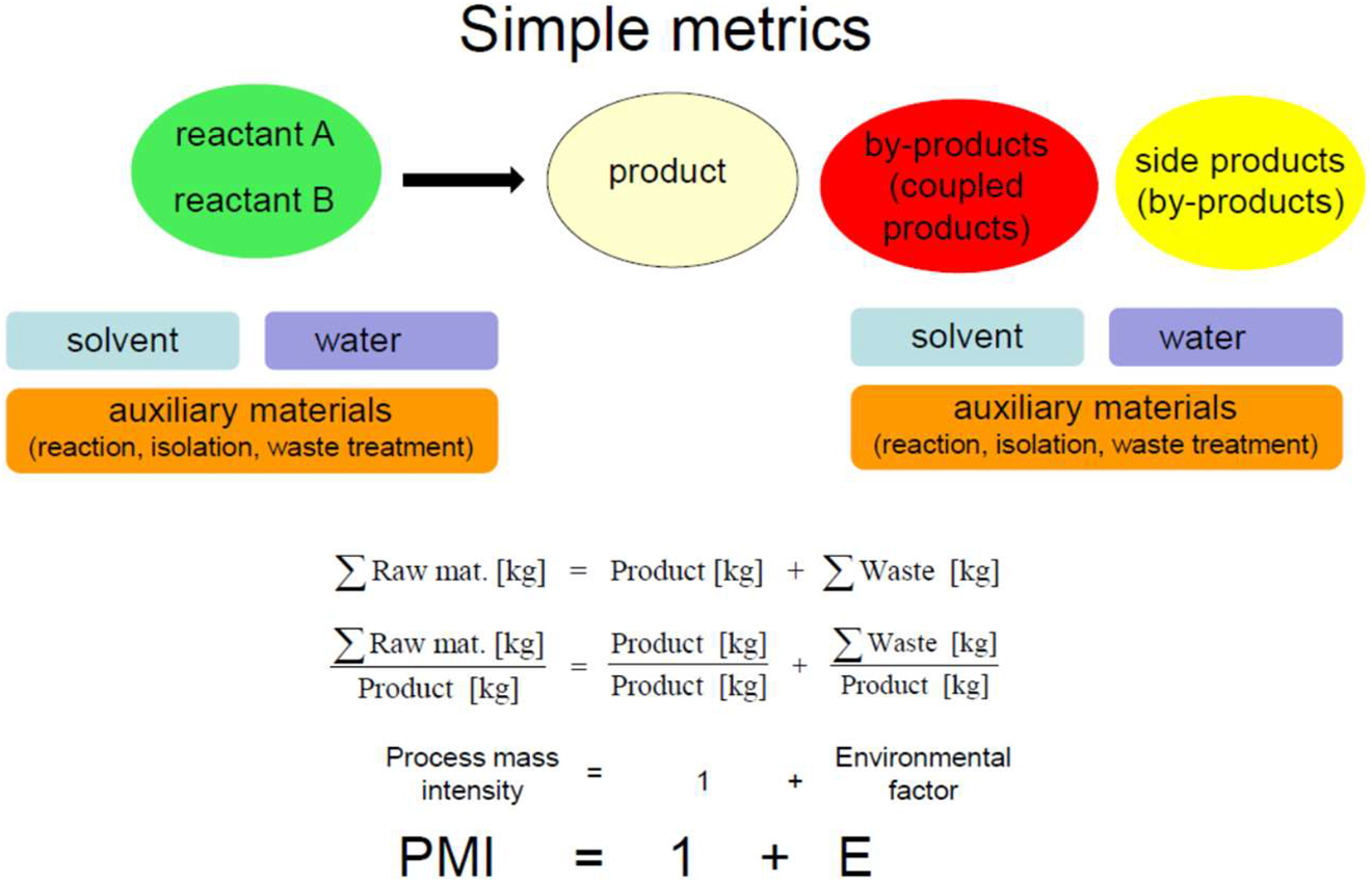
Simple metrics PMI and E-factor, which relate to input and output of a chemical synthesis.
Certainly, these metrics are very simple and are far from having the informative value of a life cycle assessment. On one hand, a lot of data and information is missing at the synthesis planning stage, and on the other hand, the E-factor and PMI can be used to draw reasonably reliable [30] and quick conclusions about the life cycle assessment. Therefore, process mass intensity is used in the pharmaceutical industry to make processes more sustainable. Consequently, data on PMI and global warming potential correlate with one another (Fig. 9).
![Fig. 9:
Correlation between PMI and Global Warming Potential/carbon footprint. Reprinted with permission from [30]. Copyright (2011) American Chemical Society.](/document/doi/10.1515/pac-2021-0326/asset/graphic/j_pac-2021-0326_fig_009.jpg)
Correlation between PMI and Global Warming Potential/carbon footprint. Reprinted with permission from [30]. Copyright (2011) American Chemical Society.
This certainly does not mean that E-factor and PMI make LCA superfluous. After all, small changes in the mass balance can have a significant impact on the global warming potential. For example, doubling the base which is used to recycle an auxiliary material during development from the laboratory to the later process resulted in a 10-fold reduction in the contribution of that auxiliary material to the global warming potential (Fig. 10). In this example the mass balance, due to a minimal change, gives no indication of a significant change that would show up in a life cycle assessment.
![Fig. 10:
Fractions of global-warming scores (% of total impact) for auxiliary and base used to recycle auxiliary at different stages of process development. See Supplementary material of reference [31] or reference [25] – Reproduced by permission of John Wiley and Sons.](/document/doi/10.1515/pac-2021-0326/asset/graphic/j_pac-2021-0326_fig_010.jpg)
However, other studies show that mass balances using E-factor and PMI agree quite well with the result of an LCA which was carried out using the Ecoindicator 95 method. Using the example of two asymmetric reduction reactions (Scheme 3), an advantage for variant B is shown both for the E-factor (Fig. 11) and for the LCA (Fig. 12), variant B resulting in fewer Eco-Points than variant A.
![Scheme 3:
Two possible syntheses (variants A and B [32]) of (R)-2-hydroxy-4-phenylbutyric acid (ethylester) [25] – Reproduced (adapted) by permission of John Wiley and Sons.](/document/doi/10.1515/pac-2021-0326/asset/graphic/j_pac-2021-0326_scheme_003.jpg)
![Fig. 11:
E-factor of the two variants A and B of the reduction reactions from Scheme 3 [25] – Reproduced (adapted) by permission of John Wiley and Sons.](/document/doi/10.1515/pac-2021-0326/asset/graphic/j_pac-2021-0326_fig_011.jpg)
![Fig. 12:
Eco-points of the two variants A and B of the reduction reactions [33] from Scheme 3. Modified reprinted from J. Clean. Prod., 7, G. Jödicke, O. Zenklusen, A. Weidenhaupt, K. Hungerbühler, Developing environmentally-sound processes in the chemical industry: a case study on pharmaceutical intermediates, 159–166, Copyright (1999), with permission from Elsevier.](/document/doi/10.1515/pac-2021-0326/asset/graphic/j_pac-2021-0326_fig_012.jpg)
Eco-points of the two variants A and B of the reduction reactions [33] from Scheme 3. Modified reprinted from J. Clean. Prod., 7, G. Jödicke, O. Zenklusen, A. Weidenhaupt, K. Hungerbühler, Developing environmentally-sound processes in the chemical industry: a case study on pharmaceutical intermediates, 159–166, Copyright (1999), with permission from Elsevier.
Another parallel between a life cycle assessment and simple metrics is shown by a comparison of several photocatalytic reactions (Fig. 13). Here, we encounter the term EATOS. EATOS [31, 34, 35] is an Environmental Assessment Tool for Organic Syntheses; a free software which can be employed to calculate E-factor and PMI, even for multi-step synthesis sequences. In addition, qualitative aspects such as toxicology can be semi-quantitatively introduced into the metrics.
![Fig. 13:
Comparison of different photocatalytic reactions, but their reaction equations are not presented here. For more information, see the literature [36]. Reprinted from Appl. Catal., B, 99, D. Ravelli, D. Dondi, M. Fagnoni, A. Albini, Titanium dioxide photocatalysis: An assessment of the environmental compatibility for the case of the functionalization of heterocyclics, 442–447, Copyright (2010), with permission from Elsevier.](/document/doi/10.1515/pac-2021-0326/asset/graphic/j_pac-2021-0326_fig_013.jpg)
Comparison of different photocatalytic reactions, but their reaction equations are not presented here. For more information, see the literature [36]. Reprinted from Appl. Catal., B, 99, D. Ravelli, D. Dondi, M. Fagnoni, A. Albini, Titanium dioxide photocatalysis: An assessment of the environmental compatibility for the case of the functionalization of heterocyclics, 442–447, Copyright (2010), with permission from Elsevier.
Mass related metrics
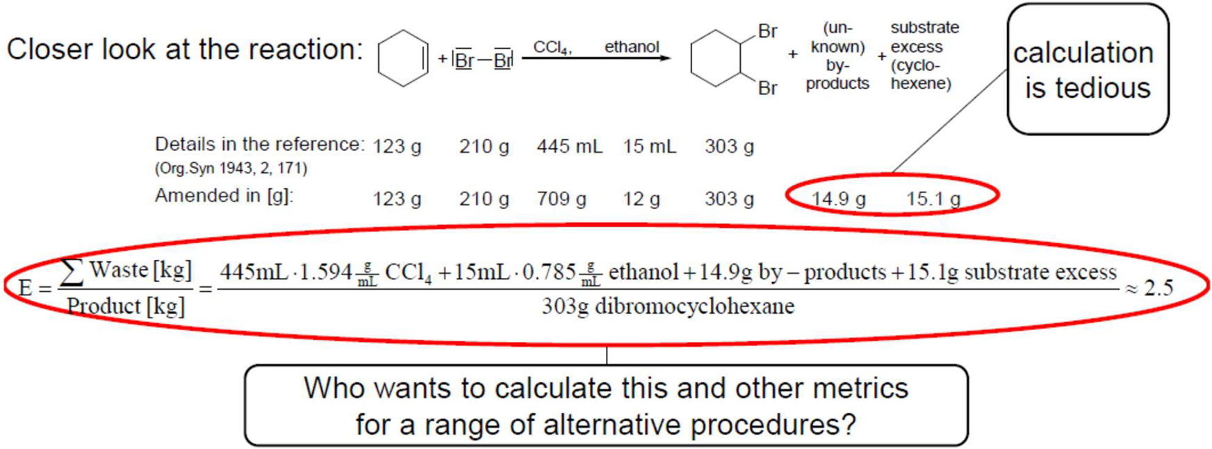
Obviously, it makes sense to demonstrate how these metrics can be determined. In Table 1 the environmental factor is first shown along with the yield and atom economy for a simple bromination reaction. Bromine is associated with hazards, which is why there are repeated efforts to carry out bromination reactions without molecular bromine and to produce it in small quantities in situ (see Synthesis 2 and 3) during the reaction. For more details about the environmental factor see Fig. 14.
Yield, atom economy, and environmental factor of three different bromination reactions.
| Yield
|
Atom economy AE
|
Environmental factor E
|
Protocol (brief version) | |
|---|---|---|---|---|
Synthesis 1 Addition of bromine to cyclohexene |
95.3 % |
100 % |
2.5 |
Cyclohexene (123 g), Br2 (210 g) 445 mL carbontetrachloride (ρ = 1.594 g mL−1) 15 mL ethanol → 303 g yield |

Synthesis 2 Addition of bromine to cyclohexene using sodium bromide and sodium perborate |
87 % |
62 % |
10.5 |
Sodium perborate (2.29 g), Cyclohexene (1.11 g) 25 mL acetic acid Sodium bromide (3.06 g) (aqueous work-up) |
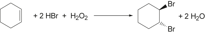
Synthesis 3 Addition of bromine to cyclohexene using hydrogen bromide and hydrogen peroxide |
86 % | 87 % | 5.8 | Cyclohexene (0.01 mol), 5 mL carbontetrachloride, 35 % hydrogen peroxide (1.9 g) 48 % hydrogen bromide (3.37 g) (aqueous work-up) |
Experimental details considered in the E-factor.
The numbers for the first reaction are noted under the reaction equation (Fig. 14), where the masses of the unknown by-products and the reactant excess are indicated as well. Of course, the calculation of the latter is a bit complicated. The ratio of waste to product is the environmental factor, which results in the value 2.5. But who wants to calculate these and other metrics for a whole range of alternative procedures? A tool is required. This could be the EATOS software. First, the stoichiometry is entered (Fig. 15). There are no by-products in this reaction. They are referred to as coupled products in the software. The masses or volumes noted in the literature are then entered in another window. If this is done for several syntheses, they can be compared in another window.
![Fig. 15:
Entering information from the protocol of a synthesis using the EATOS software [31] – Reproduced (adapted) by permission of The Royal Society of Chemistry.](/document/doi/10.1515/pac-2021-0326/asset/graphic/j_pac-2021-0326_fig_015.jpg)
Entering information from the protocol of a synthesis using the EATOS software [31] – Reproduced (adapted) by permission of The Royal Society of Chemistry.
Figure 15 is a very important figure in this article. The appeal is: use mass-related metrics! Prove the efficiency of what is done or show where there is a need for further optimization. Always show a comparison to alternatives, if they exist. How can this be done in a simple and fast manner? This figure shows how simple it is: stoichiometry, quantity and comparison – E-factor and PMI. Syntheses can also be linked together in a synthesis sequence.
When comparing these syntheses, environmental factors emerge, as Fig. 16 demonstrates. For example, a large amount of solid waste becomes apparent, and the use of bromine may still be the best option. Costs of raw materials can also be entered in order to receive an overview of the raw material costs, and to see if optimizations are necessary (Fig. 17). EATOS can be used for this purpose, as already shown in Fig. 7; even for complex synthesis sequences. Once again: what about the hazards of bromine? How can these be considered? More about this later. There are currently many variants to avoid molecular bromine (Fig. 18). On the left side, there are alkenes and the bromination products. There are basically three methods. The use of molecular bromine, employing carrying substances or producing it in situ, as already demonstrated (entry 2 and 3 in Table 1, Figs. 15 and 16). The methods shown here will not be discussed in detail (see reference [37]) – there are quite a few. Sometimes it seems odd that a carrying system is used in order to prevent bromine, where bromine is used for recycling (entry 9b and 11, Fig. 18). On a note, a potential possibility is the conversion with hydrogen bromide (entry 20, Fig. 18).
![Fig. 16:
Environmental factor E. The right hand side shows a zoomed presentation in order to make coupled and by-products better visible (Coupled products are also called by product, and by-products are also called sideproducts.) [31] – Reproduced by permission of The Royal Society of Chemistry.](/document/doi/10.1515/pac-2021-0326/asset/graphic/j_pac-2021-0326_fig_016.jpg)
Environmental factor E. The right hand side shows a zoomed presentation in order to make coupled and by-products better visible (Coupled products are also called by product, and by-products are also called sideproducts.) [31] – Reproduced by permission of The Royal Society of Chemistry.
![Fig. 17:
Substance amounts and costs for the production of dibromocyclohexane [31] – Reproduced by permission of The Royal Society of Chemistry.](/document/doi/10.1515/pac-2021-0326/asset/graphic/j_pac-2021-0326_fig_017.jpg)
Substance amounts and costs for the production of dibromocyclohexane [31] – Reproduced by permission of The Royal Society of Chemistry.
![Fig. 18:
Further methods for electrophilic bromination of alkenes. The references shown here are those from the literature [37] – Reproduced by permission of John Wiley and Sons.](/document/doi/10.1515/pac-2021-0326/asset/graphic/j_pac-2021-0326_fig_018.jpg)
Further methods for electrophilic bromination of alkenes. The references shown here are those from the literature [37] – Reproduced by permission of John Wiley and Sons.
Figure 19 shows the environmental factor, including a zoomed figure. There is a substantial use of solvents and the formation of large quantities of by-products. The lesson is clear: scientific ambition should not focus on single issues (e.g. ‘toxic bromine’) and neglect the big picture. Metrics should be used.
![Fig. 19:
E-factor of electrophilic bromination of alkenes (Fig. 18). The large diagram is a zoomed version of the small one [37] – Reproduced by permission of John Wiley and Sons.](/document/doi/10.1515/pac-2021-0326/asset/graphic/j_pac-2021-0326_fig_019.jpg)
Another example is the synthesis of alkenes from simple basic chemicals, e.g. alkenes, alkynes, ketones and so on. Figure 20 shows the environmental factor of more than 20 methods for the production of tri- and tetrasubstituted double bonds consisting of up to six reaction steps. The synthesis with the most waste is the Julia Lythgoe method, while the best method is the metathesis. Then there is a three component reaction, which is also very good. Otherwise, there are typical alkene synthesis methods, e.g. the Heck – synthesis, the McMurry variant, Barton–Kellogg, Wittig, for which a catalytic variant is also shown here. Four examples of geminal dihalides are listed here, which coincidentally are the starting material for synthesis 11. The coupling of vinyl bromide is represented here several times, e.g. starting from a disubstituted alkene. However, what if previous reaction steps are integrated? The next two variants of entry 19 start with an aldehyde and a haloalkane, i.e. a Wittig synthesis. The amount of waste produced increases accordingly. Here, of course, the problem of a mass balance becomes apparent. Which stage in the synthesis sequence do you go back to if a fair comparison is to be made? At the same time, alternatives of preceding syntheses can always be considered. Here, in example 19b and 19c two different bromination reactions are considered. This consideration can be extended to other substances in the synthesis. Example 27b integrates the synthesis of the catalyst from entry 27a. Therefore, well-founded decisions must be made as to how far the scope of the investigation is to be set. When considering alternative variants, it may also be possible to identify efficient methods or synthesis concepts. Is the use of magnesium organyles sensible? Or of zinc organyles? Or is the use of alkynes particularly efficient? The solvent amounts are listed separately using numbers because the values are exorbitantly high in some cases. When integrated into the bar chart, they would have covered the other synthesis details. In this respect, Fig. 20 shows a PMIRCCA (for reagents, reactants, catalyst and auxiliary materials) graphically, while the number for the PMISolv (for solvent) is noted above, visually distinguishing between values from 0 to 100, from 100 to 1000, and above 1000. Since the syntheses are not optimized, the quantities involved are sometimes enormous. This means, that sometimes reasonable estimates should be made. We did this, for example, for a comparison [38] of a biocatalytic vs. a chemical synthesis of an enantiomerically pure ß-amino acid.
![Fig. 20:
Mass efficiency of alkene syntheses with tri- and tetrasubstituted double bonds. For reaction equations (up to seven steps per method) and details see the literature. Reprinted (adapted) with permission from [28]. Copyright (2017) American Chemical Society.](/document/doi/10.1515/pac-2021-0326/asset/graphic/j_pac-2021-0326_fig_020.jpg)
Mass efficiency of alkene syntheses with tri- and tetrasubstituted double bonds. For reaction equations (up to seven steps per method) and details see the literature. Reprinted (adapted) with permission from [28]. Copyright (2017) American Chemical Society.
Incidentally, when comparing synthesis methods when arbitrary reactants and products are considered in the literature, the difference in molar masses can have an impact on the PMI comparison. The product molecule, with its mass produced, is the crucial reference for the PMI. This was also pointed out in a recent [39] publication. I would suggest that in such cases a representation in kg mol−1 and not only in kg kg−1 is considered, as we have done for the alkene syntheses, see Fig. 21. The conversion is simple: PMI in kg mol−1 = PMI in kg kg−1 · MW (product) in g mol−1. It is exemplarily illustrated in Fig. 22.
![Fig. 21:
Demonstration of Fig. 20 in the unit kg mol−1. Reprinted (adapted) with permission from [28]. Copyright (2017) American Chemical Society.](/document/doi/10.1515/pac-2021-0326/asset/graphic/j_pac-2021-0326_fig_021.jpg)
![Fig. 22:
Determination of PMI in the unit kg mol−1: the mass of coupled products (2.7315 kg kg−1) of the reaction in entry 1 (Fig. 20) is exemplarily multiplied by the molar mass of the product (138.14 g mol−1) of entry 1 to obtain, with all other values, a plot as in Fig. 21. Reprinted with permission from [28]. Copyright (2017) American Chemical Society.](/document/doi/10.1515/pac-2021-0326/asset/graphic/j_pac-2021-0326_fig_022.jpg)
Determination of PMI in the unit kg mol−1: the mass of coupled products (2.7315 kg kg−1) of the reaction in entry 1 (Fig. 20) is exemplarily multiplied by the molar mass of the product (138.14 g mol−1) of entry 1 to obtain, with all other values, a plot as in Fig. 21. Reprinted with permission from [28]. Copyright (2017) American Chemical Society.
Meanwhile several tools exist (Fig. 23), for some comparisons see references [40], [41], [42]. In industry, for example, l’Oréal uses Eco-footprint [43], which was inspired by EATOS [31, 34, 35], and Hoffmann La Roche [44] uses ChemPager, and Bristol-Myers Squipp [45] uses a Process Greenness Scorecard. A consortium of academics, pharmaceutical companies and SMEs developed the CHEM21 toolkit [46] and a scoring method was developed for the 12 green chemistry principles [47], a so-called [48] greeness grid. These tools take into account not only mass balances, but also qualitative criteria [41] on environmental, health and safety concerns. For example, CHEM21 [46] refers to a safety concept [49] used in a number of pharmaceutical companies and parts of which can also be easily integrated [50] into university education.
![Fig. 23:
Critical evaluation of published algorithms. Reprinted with permission from [40, 41]. Copyright (2016) American Chemical Society.](/document/doi/10.1515/pac-2021-0326/asset/graphic/j_pac-2021-0326_fig_023.jpg)
Another interesting tool is the PMI calculator by ACS (Fig. 24). It contains typical PMIs of real production processes for many reactions. It is thus possible to obtain an overview of the total PMI that can realistically be expected for a synthesis sequence.
![Fig. 24:
Example for the second application step of the PMI calculator [51] for a synthesis sequence of eight syntheses A to H. The PMI calculator is assisted by predictive analytics and historical data; https://acsgcipr-predictpmi.shinyapps.io/pmi_calculator/.](/document/doi/10.1515/pac-2021-0326/asset/graphic/j_pac-2021-0326_fig_024.jpg)
Example for the second application step of the PMI calculator [51] for a synthesis sequence of eight syntheses A to H. The PMI calculator is assisted by predictive analytics and historical data; https://acsgcipr-predictpmi.shinyapps.io/pmi_calculator/.
However, no detailed weak-point analysis can be carried out, e.g. what exactly provides a high PMI contribution in a synthesis. In this respect, this tool by itself is not sufficient.
Metrics for environmental issues
Among the qualitative aspects considered in a life cycle assessment (see above) are the PBT-criteria (persistence, bioaccumulation, toxicity), which will be considered separately here. (Commercial [52]) persistent, bioaccumulative and/or toxic chemicals are the focus of the EU Risk rAnking Method (EURAM [53]), which even takes into account their distribution in the environment. The BASF-method [8, 54] applies this concept, but keeps evolving and modifying it. However, as many of the data inputs needed were typically missing in EINECS list of existing chemicals, ranking methods have been examined and a tool called Decision Analysis by Ranking Techniques (DART [55]) was developed, which is one of the publicly accessible QSAR [56]-tools developed by the European [57] Commission’s Joint Research Centre. First, using QSAR-tools, e.g. of the US-EPA, concern scores for chemicals are determined for each of the PBT-criteria (Table 2).
Conversion of P, B and T predictions in different [55] levels of concern.
| Persistence | BCFa | Toxicityb | Concern Score |
|---|---|---|---|
| Non-linear model < 0.5 or (MITI non-linear model < 0.5 and Ultimate biodegradation < 2.2) | 2000 < BCF | LC50 ≤ 1 | 4 |
| 2.2 ≤ Ultimate biodegradation < 3 | 1500 < BCF ≤ 2000 | 1 < LC50 ≤ 10 | 3 |
| 3 ≤ Ultimate biodegradation < 3.5 | 1000 < BCF ≤ 1500 | 10 < LC50 ≤ 100 | 2 |
| 3.5 ≤ Ultimate biodegradation | BCF ≤ 1000 | 100 < LC50 | 1 |
-
aBCF, bioconcentration factor; bLC50 = lethal concentration for 50 % of tested population.
In the following, a method will be presented which is based on the idea of DART and the concern scores and enables the determination of weighting factors for substances with regard to their PBT-property. Two of the seven ranking methods will be introduced briefly: the desirability and the utility function. Figure 25a shows the function (1) referring to a concern score (Table 2).
where P = persistence, B = bioconcentration factor, T = toxicity, i.e. desirabilities exist for P, B, and for T.
Another type, for example an exponential function instead of a linear function could have been considered just as well (Fig. 25b).
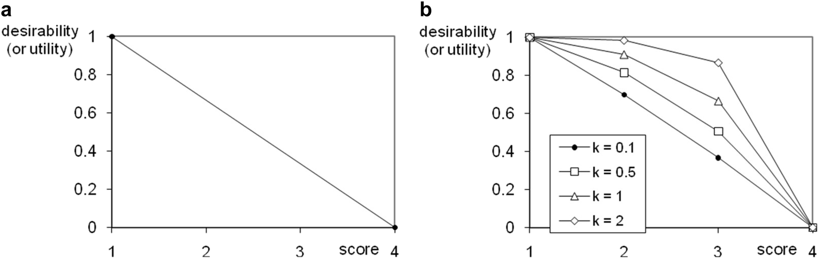
Inverse relationship between the ranking score and its desirability (or utility). a) Linear function (equation (1)) and b) exponential functions (eq. (4)) assign ranking values from 0 to 1 to the concern scores. The Supplementary material includes a corresponding Excel file (j_pac-2021-0326_suppl_003_DART_example.xls).
According to the scores, corresponding desirability (or utility) values have to be determined for each PBT-criteria. These three results have to be combined to the overall desirability (or utility). Therefore, weighting factors are necessary, e.g. 1/3 for each criteria in order to consider them to the same extent, and are combined in a geometric (2) or arithmetic (3) means.
where D is the overall desirability, U is the overall utility and scoreP etc. are the scores for persistence, bioaccumulation and toxicity.
Once D has been calculated for each element, these can be ranked according to their D value. The element with the highest D can be selected as the best one [55], if its D value is acceptable. A Desirability scale is shown in Table 3.
| Scale of D | Quality evaluation |
|---|---|
| 1.00 | Improvement beyond this point has no preference |
| 1.00–0.80 | Acceptable and excellent |
| 0.80–0.63 | Acceptable and good |
| 0.63–0.40 | Acceptable but poor |
| 0.40–0.30 | Borderline |
| 0.30–0.00 | Unacceptable |
| 0.00 | Completely unacceptable |
Therefore, a value close to 1 indicates a good rating and close to 0 indicates a poor rating. These values can be used for an evaluation of problematic substances by multiplicative weighting, if scaled exactly the other way round. The overall PBT-hazard ranking can simply be 1 – D (or 1 – U), i.e. a PBT-hazard ranking of 0 is perfect, whereas 1 is the worst value. Thus, problematic substance quantities are maintained in quantity by a factor of 1, while quantities of less problematic substances are decreased by values closer to 0. This brings the problematic substances into focus. As can be seen in Table 4 the PBT-hazard score according to the desirability is more sensitive than according to utility: if only one criteria shows the concern score 4 the hazard score will be 1.
Determination of PBT-hazard scoresf – some examples, considering a) a linear function or b) an exponential function.
| a) a linear function | or b) an exponential function | |||||||||||
|---|---|---|---|---|---|---|---|---|---|---|---|---|
| Scoresa | Desirability (or utility)b | PBT-hazard score | Desirability (or utility)e | PBT-hazard score | ||||||||
| P | B | T | P | B | T | Utilityc,f | Desirabilityd,f | P | B | T | Utilityc,f | Desirabilityd,f |
| 1 | 1 | 1 | 1 | 1 | 1 | 0 | 0 | 1 | 1 | 1 | 0 | 0 |
| 1 | 2 | 3 | 1 | 0.667 | 0.333 | 0.333 | 0.394 | 1 | 0.910 | 0.665 | 0.142 | 0.154 |
| 2 | 2 | 3 | 0.667 | 0.667 | 0.333 | 0.444 | 0.471 | 0.910 | 0.910 | 0.665 | 0.172 | 0.180 |
| 1 | 1 | 4 | 1 | 1 | 0 | 0.333 | 1 | 1 | 1 | 0 | 0.333 | 1 |
| 1 | 2 | 4 | 1 | 0.667 | 0 | 0.444 | 1 | 1 | 0.910 | 0 | 0.363 | 1 |
| 1 | 4 | 4 | 1 | 0 | 0 | 0.667 | 1 | 1 | 0 | 0 | 0.667 | 1 |
| 4 | 4 | 4 | 0 | 0 | 0 | 1 | 1 | 0 | 0 | 0 | 1 | 1 |
-
aConcern scores of seven fictitious substances were assigned according to information on their biodegradability, bioconcentration and LC50 data using Table 2; baccording to eq. (1); caccording to 1 – U = 1 – eq. (3); daccording to 1 – D = 1 – eq. (2); eaccording to eq. (4) with k = 1; fThe higher, the worse. The numbers in bold are the PBT-hazard scores, with which substance masses can be weighted according to their hazard potential. They result from the values of the three previous columns for P, B and T respectively. The Supplementary material provides a corresponding Excel file (j_pac-2021-0326_suppl_003_DART_example.xls).
A similar ranking and (flexible) weighting system already exist with EATOS. However, DART is supposed to find a broad consensus because it is offered on the official internet pages of the European Commission. Alternative synthetic variants could be compared by allocating all substances used to the PBT-hazard scores. Aside from this hazard identification concept, emissions from the chemical production could be weighted by the PBT-hazard score by multiplication. For example, substance A, which is emitted with 0.005 kg per kg of product and with a PBT-hazard score of 0.180, will be weighted to 0.005 · 0.18 = 0.009. Substance B obtains a weighted value of, let’s say, 0.003. The sum of the results for A and B, here 0.009 + 0.003 = 0.012 may provide a clue about persistence, bioaccumulation and toxicity potential of alternative syntheses or synthetic sequences. If high concern scores should be taken into account to a higher degree, an exponential function (Fig. 25b) could be preferable. Thus, a chemical with P = 2, B = 2, and T = 3, its PBT-hazard score (utility) according to the linear function (eq. (1)) being the same as that of a chemical with P = 1, B = 2, and T = 4 (see two times 0.444 in Table 4a), receives a lower PBT-hazard score (utility), when an exponential function (Fig. 25b) is used (see 0.172 vs. 0.363 in Table 4b). By varying the parameter ‘k’ in eq. (4) the importance of concern scores 2 and 3 can be modified (see Fig. 25b) with regard to a sensitivity analysis. The higher the parameter ‘k’, the less the effect of substances with concern scores of 2 or 3. Their hazard scores then decrease compared to substances with a concern score of 4. Equation (4) was formed so that it passes through the corner points (0|1) and (4|0) (see Fig. 25b).
where score is the concern score (Table 2) and k is a parameter with which the relative contribution of concern scores 1 to 4 to a PBT-assessment can be modified (Fig. 25b).
Emissions which are to be assessed with the PBT-hazard score, are not known in early synthesis design. However, if measurement data or meaningful values [59] cannot be determined by taking a closer look at individual technical components of a process, such as a distillation process, the Technical Guidance Document [60] of the European Commission could be an interesting source for standard emission values depending on production volume, vapour pressure and water contact (see ESI Table 18 for an example).
Metrics for health hazards
Approaches in the literature
Health hazards concern qualitative issues such as a substance’s toxicity and how likely exposure to it would be. Despite the difficulty of a quantification, it is the goal of a range of approaches in literature, see e.g. reference [61]. Besides the methodology [34] being implemented in EATOS (see Fig. 26, or, e.g. ref. [62, 63]), there are many others, some of which will be briefly introduced (Figs. 27, 28, 29, and Table 5).
![Fig. 26:
Example of the use of EATOS to semiquantitatively incorporate qualitative criteria such as toxicology, for the input (EI_in) and output (EI_out) of syntheses to be compared in an evaluation with a potential environmental impact (PEI). The diagrams refer to the synthesis methods shown in Fig. 7. Reproduced from Ref. [29] with permission from The Royal Society of Chemistry.](/document/doi/10.1515/pac-2021-0326/asset/graphic/j_pac-2021-0326_fig_026.jpg)
Example of the use of EATOS to semiquantitatively incorporate qualitative criteria such as toxicology, for the input (EI_in) and output (EI_out) of syntheses to be compared in an evaluation with a potential environmental impact (PEI). The diagrams refer to the synthesis methods shown in Fig. 7. Reproduced from Ref. [29] with permission from The Royal Society of Chemistry.
![Fig. 27:
Determination of the potential chemical risk [65] according to the literature [66] Reprinted (adapted) with permission from [65]. Copyright (2007) American Chemical Society.](/document/doi/10.1515/pac-2021-0326/asset/graphic/j_pac-2021-0326_fig_027.jpg)
![Fig. 28:
Relevant categories in ‘Control of Substances Hazardous to Health’ (COSHH [67]) regulations in Great Britain. For further reading see e.g. [68], [69], [70].](/document/doi/10.1515/pac-2021-0326/asset/graphic/j_pac-2021-0326_fig_028.jpg)
![Fig. 29:
a) Scoring of acute toxicity [71] in the BASF-method [8, 72] and b) determination of index values for irritation, chronic toxicity and mobility hazard [64] in the EHS-method.](/document/doi/10.1515/pac-2021-0326/asset/graphic/j_pac-2021-0326_fig_029.jpg)
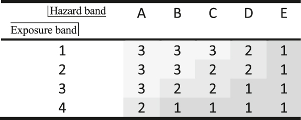
Priority bands in the Stoffenmanager. Hazard: A = lowest hazard and E = highest hazard. Exposure: 1 = lowest exposure and 4 = highest exposure. Overall result: 1 = highest priority and 3 = lowest priority [73]. The hazard band is determined via COSHH (see Fig. 28).
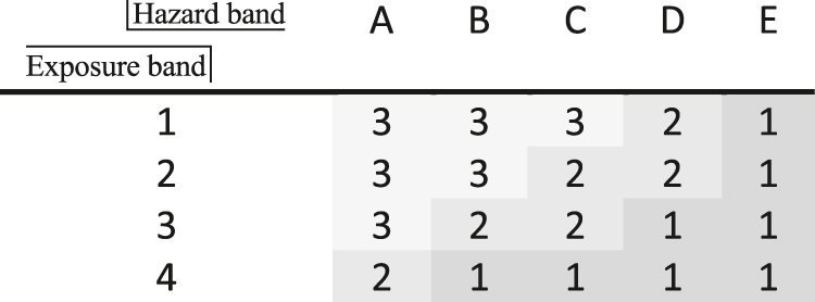 |
All methods have in common that toxicological effects are somehow ranked or grouped. In this case, H-statements (the former R-phrases) are used optionally (EHS-method [64]) or exclusively. It is interesting that the EHS-method (Fig. 29b) does not consider acute toxicity amongst health but rather as a part of safety hazards. Instead, it refers to corrosiveness and chronic toxicity. Only the EATOS-procedure and the BASF-method (Fig. 29a) use the scores to weigh absolute substance quantities. In contrast to the other approaches the consideration of exposure potential, i.e. of the probability of ‘contact’ with a substance, is missing. Exposure depends on a) how often hazardous substances are applied (see frequency class (Fig. 27), b) how concentrated substances are in mixtures (see quantity level (Fig. 27)), c) how much of a substance is used (Fig. 28), d) how volatile or dusty a substance is (Figs. 28 and 29b and e) which physical substance properties and technological prerequisites are given (see Fig. 29 and control approach in Fig. 28). The exposure band (Table 5) in the Stoffenmanager takes a range of parameters into account, e.g. room size, ventilation, local control measures, protection measures, handling conditions, duration of application, and exposure frequency. Due to this spectrum of influencing factors, which have scientifically been examined, the Stoffenmanager can be considered to be an appropriate concept also for chemical production processes. Necessary adjustment measures are described in the following chapter.
Application of the Stoffenmanager to chemical processes
The idea behind Table 5 is to identify which substances require measures to transform their application from a high priority (values 1 and 2) to low priority (value 3). Also, highlighting specific substances in combination with e.g. technological constraints is desirable and appropriate for hazard minimization during chemical processes. However, to receive an overall picture of the health situation of a (multistep) production process for a comparison to alternative procedures, the simple addition of something such as ‘health scores’ could be helpful. Thus, in early synthesis design, where a range of alternatives have to be taken into account, a final ‘health index’ allows for a pragmatic comparison. The classification of 3 to 1 is somewhat rough, which is why a transformation into more differentiated scores can be considered reasonable. Therefore, the Stoffenmanager could be adapted in this regard. An example is given within Table 6, showing a trend similar to that given in Table 5: from ‘good’ (top left) to ‘bad’ (downright).
Health scores (for inhalation hazard) according to hazard and exposure band.

|
A | B | C | D | E |
|---|---|---|---|---|---|
| 1 | 0.0078125 | 0.015625 | 0.03125 | 0.0625 | 0.125 |
| 2 | 0.015625 | 0.03125 | 0.0625 | 0.125 | 0.25 |
| 3 | 0.03125 | 0.0625 | 0.125 | 0.25 | 0.5 |
| 4 | 0.0625 | 0.125 | 0.25 | 0.5 | 1 |
-
The higher the value the more problematic the substance. The difference within the hazard and exposure band cannot be substantiated scientifically and is more or less arbitrary. In this example a substance in a hazard band is considered twice as problematic as a substance in a lower hazard band. The same is valid for the exposure bands. The application of these health scores is flexible and should be part of a sensitivity analysis, see ESI Table 12 and ESI file j_pac-2021-0326_suppl_004_STOFFENMANAGER_MODIFICATION_construction_of_health_scores.xls.
The factor from one hazard band to the next is flexible and follows the procedure shown in Table 14 (see ESI). An example for utilization of the hazard band in order to determine the hazard potential can be found in the literature [38]. A comparison [38] with other assessment methodologies builds confidence in the concept considering the hazard band [67] of COSHH. For more details concerning health score, see the ESI.
In the Stoffenmanager, the exposure pathway via skin is considered separately. Health risk scores are determined for local and systemic health effects (see Tables 9 and 14 in the literature [74]). Similar to Fig. 29 scores from 1 to 10 highlight the problematic area: 1 is best and 10 is worst case. As described for inhalation hazard, an overall health index can be considered to be more straightforward. Ideally, the assessment of inhalation exposure should be combined with skin exposure. Therefore, an allocation of the numbers 1 to 10 to the same value range of the health score for inhalation hazard is proposed, e.g. 0.0078125 to 1 (Table 6), to allow for a simple addition. The procedure is described specifically in Table 15 (see ESI). However, a scientific procedure which shows how to combine inhalation with skin hazard does not exist. This adaptation of the Stoffenmanager can be considered to be a pragmatic approach.
The Stoffenmanager aims to make clear where measures should be taken, e.g. local control measures or ventilation. Ideally, health scores will decline correspondingly to an acceptable value. However, in early synthesis design, when a range of synthetic variants are taken into account, a detailed (and time demanding) look at all these parameters (see chapter ‘Approaches in the literature’) is not mandatory. Possibly, the default values could be applied to all processes to be compared. Thus, only parameters such as how diluted or how volatile a substance is will contribute to the assessment. In a computer tool this information is automatically accessed via the mass balance and a substance data bank. A detailed view is worthwhile for synthetic variants which are interesting and maybe for those where appropriate measures are known and can be considered immediately. The ESI offers a case study in an Excel tool to illustrate the processing of data. In this preliminary tool vapour pressure still has to be entered manually. The result will be presented in the context of a case study (next chapter).
Two parameters which are implemented within the Stoffenmanager consider whether substances are handled in closed containers or with high speed and whether there is mechanical treatment or hand tool dispersion. They are called ‘Handling’ and ‘Task group’. A chemist would rather turn to REACH Process Categories (PROC, see Table 1 in the document [75]) of the European Centre for Ecotoxicology and Toxicology of Chemicals (ECETOC). For example, PROC 2 is “Use in closed, continuous process with occasional controlled exposure” and PROC 8 is “Transfer of chemicals from/to vessels/large containers at non dedicated facilities”. Thus, a fixed allocation of PROCs to ‘Handling’ would be desirable, but it does not exist. However, the developer of the Stoffenmanager made a suggestion for Handling categories for PROCs. An assignment has been developed to provide default values. I have therefore developed an allocation to deliver default values.
Case study
Oils and fats [76, 77] are considered to be a sustainable [78, 79] source of feedstocks [19] for the chemical industry, among other things. The utilization of waste materials that are generated in the course of their exploitation is highly desirable. For example, waste olive leaves accumulated during olive harvest can be extracted to obtain oleuropein aglycon. This physiologically active [80], [81], [82], [83] substance can be used as a cross-linking material for gelatine. An alternative (Table 7) substrate for this purpose is glutaraldehyde (Scheme 4).
Two alternative feed stocks for the production of a cross-linking material for gelatine: glutaraldehyde and oleuropein aglycon.
| Alternative A | Alternative B | |
|---|---|---|
| Raw material | Glutaraldehyde | OP-Agly |
| Source | Crude oil | Olive leaves |
| Production via | Chemical synthesis | Extraction |
| Structure |

|
|
![Scheme 4:
Synthesis sequence to glutaraldehyde and data collection using Ecoinvent and Umberto [84]. Ref. [85] – Reproduced by permission of John Wiley and Sons.](/document/doi/10.1515/pac-2021-0326/asset/graphic/j_pac-2021-0326_scheme_004.jpg)
Besides mass flows, energy demand was calculated considering the stoichiometric equation reaction temperature, reaction pressure, compression of liquids, enthalpy of evaporation, drying, etc. However, there are, of course, uncertainties because only literature and not actual process data were considered. The synthesis of glutaraldehyde [85] (Scheme 4) was modelled (ESI Fig. 36) using the software Umberto®. As a result, a Sankey diagram (ESI Fig. 37) was obtained. The total CED is 91.8 MJ kg−1 (ESI Table 20b). The environmental impacts concerning oleuropein aglycon were also determined on the basis of mass flow. The results, however, are confidential and cannot be demonstrated. At least some principle findings can be reported resulting from the process model (lab scale!): the yield of OP-Agly has to be increased. The water demand has to be reduced, because heating is energy intensive. The solvent ethanol should be applied more efficiently. Currently, 120 L are used to extract 2.7 kg of product. Steam demand during evaporation of the solvent should be reduced, and the solvent should be worked-up and reused. Olive leaves should be manufactured regionally. This case study illustrates the expenses linked to the requirements of a life cycle assessment. Especially when data are missing in the data bases such as the Ecoinvent data base, and processes have to be modelled e.g. in Umberto® (see Scheme 4, ESI Fig. 36 and ESI Fig. 37). Researching missing data in the literature to that extent, as has been done for glutaraldehyde (Scheme 4), promotes the assumption that life cycle assessments will not receive the status of a standard procedure in early synthesis design. A pragmatic procedure could be done by estimations. An example is the EstiMol tool (Table 8), which models the cumulative energy demand (CED), the global warming potential (GWP) and the Ecoindicator 99 for a range of chemicals. The CED for glutaraldehyde, which was determined [85] as part of the life cycle assessment (ESI Table 20b, using CML 2001 [86]), amounts to 91.8 MJ kg−1. Interestingly, this result lies well within the calculation of the EstiMol [17] tool (116.8 ± 42.57, Table 8).
Modelling of the cumulative energy demand, global warming potential and of the Ecoindicator 99 points using the EstiMol [17] tool (Fig. 1).
| CED | GWP | EI99 | ||||
|---|---|---|---|---|---|---|
| Mean | σa | Mean | σa | Mean | σa | |
| Glutaraldehyde | 116.8 | 42.57 | 3.701 | 2.196 | 0.3581 | 0.1718 |
-
aσ = standard deviation.
The system boundary is also a topic for health as well as safety aspects. The industrial equipment has to ensure a safe final process without any compromises to health standards. Respective persons in charge strive for an appropriate organizatorial and technical solution. Although the upstream chain is in fact suggested in the Ecoefficiency analysis of the BASF [71], the focus of occupational health and safety practitioners and corresponding chemical engineers of a company normally lies with their own industrial site and not with their suppliers. Nevertheless, the health hazard profiles for the production of glutaraldehyde and of oleuropein aglycon should be presented (Fig. 30) beginning with crude oil. Default values (ESI Table 21) concerning, for example, room size and local controls were considered to determine the health scores. The comparison of glutaraldehyde and oleuropein aglycon production (Fig. 30a, b vs. c) reveals that the multistep procedure (Scheme 4) shows a much higher health hazard potential. This results from several subprocesses considering many more substances than the extraction of the olive leaves. One detail that should be mentioned here is the eye-catching subprocess 1 of Fig. 30c. Naphta, an obvious carcinogenic substance, is used for the production of the extraction solvent ethanol. Details of the glutaraldehyde profile can be identified from the corresponding Excel file (Supplementary material).
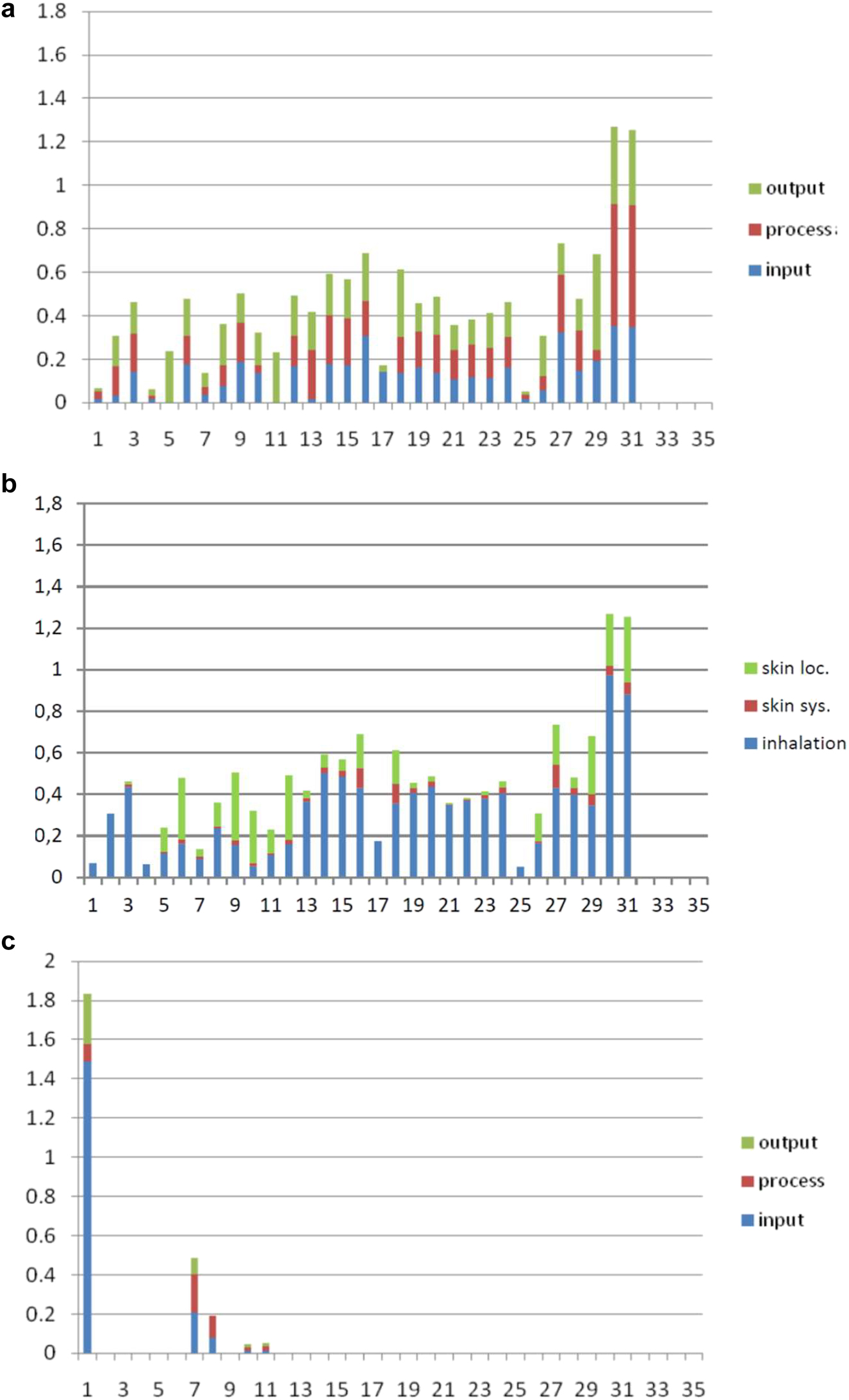
Health scores (y-axis) for the production of a), b) glutaraldehyde (31 process steps, x-axis) (see j_pac-2021-0326_suppl_005_STOFFENMANAGER_MODIFICATION_example_glutaraldehyde.xlsx; tab RESULT) and c) oleuropein aglycon (11 process steps) according to the application of the Stoffenmanager (see chapter showing Table 6) (see j_pac-2021-0326_suppl_006_STOFFENMANAGER_MODIFICATION_example_oleuropein_aglycon.xlsx; tab RESULT). Whereas a) is sorted according to whether substances appear during input, process or output, b) presents skin (local, systemic) and inhalation hazards. No special conditions were considered. Default values (ESI Table 21) were assumed for all processes.
Besides the application of the Stoffenmanager, a toxicity assessment according to the BASF method was performed (Fig. 31). However, the assessment was performed only regarding the process and without consideration of the product application, for which the BASF method concedes a contribution of a certain ratio of the overall assessment result. Interestingly, the results are inconsistent when compared to one another (Fig. 31a). If naphta is neglected, because, for example, ethanol is produced from renewable feedstocks, at least the trend is similar (Fig. 31b). However, the qualitative difference of the results is still striking. Obviously, the evaluation methodologies show their differences: In the BASF method, substance quantities are considered, whereas in the modified substance manager concept, exposure information is used as well. The hazard banding according to the H-statements (formerly R-phrases) is at least not likely to be the reason for the clearly different result in Fig. 31b – at least the example in literature [38] shows broad consistency (compare columns ‘COSHH (b = 2)’ and ‘BASF’ in Fig. 4 of the literature [38]).
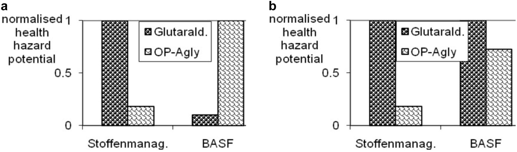
Normalised health profile for the production of glutaraldehyde and oleuropein aglycon (see ESI Table 19). a) with and b) without consideration of naphta for oleuropein aglycon production.
Education: example for the joint presentation of mass related metrics and hazard statements
Another integration of health hazards is presented on the website of a lab course called “Sustainability in the organic chemistry lab course” (Figs. 32 and 33). Here, synthesis protocols for the chemical laboratory in education are offered. As an example, another bromination reaction is shown. The reaction equation is presented alongside hazard notes. The data availability is highlighted in color (Fig. 33), indicating whether toxicity or ecotoxicity data are available. Effect factors of an official method are also highlighted in color and displayed in the process mass intensity (PMI). Didactic guidance on how to address metrics [31] in teaching and more experiments [87] can be found in the literature.
![Fig. 32:
Website of the “Sustainability in the organic chemistry lab course” [88, 89] (NOP, Nachhaltiges Organisch-chemisches Praktikum).](/document/doi/10.1515/pac-2021-0326/asset/graphic/j_pac-2021-0326_fig_032.jpg)
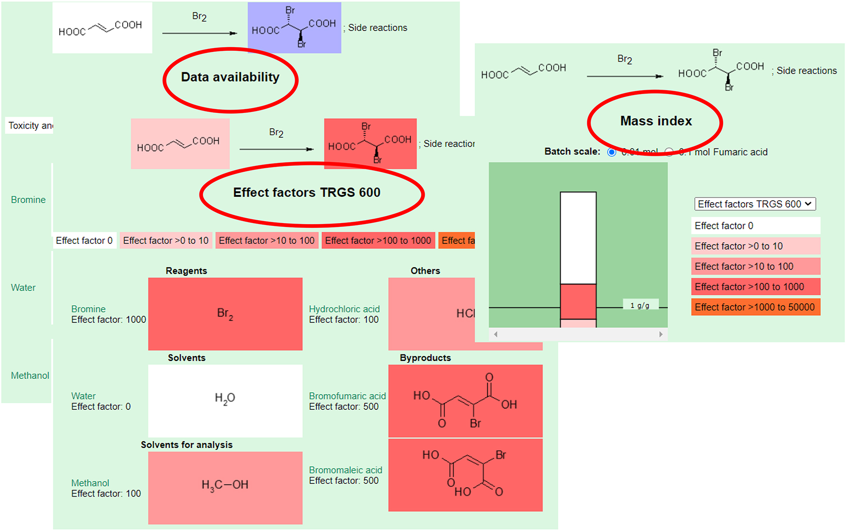
Quantitative and qualitative aspects, which are presented for a synthesis protocol of a bromination reaction on the website of the NOP (Fig. 32).
Concluding remarks
The presentation of metrics for environmental aspects as well as for the consideration of health and safety [90] aspects can only remain incomplete. There are numerous approaches [8, 42, 54, 61, 65, 91], [92], [93], [94], [95], [96], [97], [98], [99], [100], [101], [102], [103], [104], [105], [106], [107], [108], which cannot be sufficiently recognized here. Correspondingly, I have set a focus on those methodologies which I would like to see implemented in an automatic software tool that is helpful for the chemist in early synthesis design. This tool would also include an aggregation method for the rubric environment, which contains the other categories of LCA, e.g. greenhouse potential, acidification potential, land use, etc. This could not be discussed in the lecture due to time constraints and is therefore missing here. The presentation of alternative methodologies is meant to impart an impression of related aspects. Of course, this remains a subjective view. Table 9 shows some pros and cons of considered methods, concepts and metrics.
Pros and cons of methods, concepts and metrics considered.
| Method/concept/metrics | Pro | Contra |
|---|---|---|
| PMI and E | Easy and quick determination: | Quality of data basis: |
|
|
|
| Expressiveness/reliability: | ||
|
|
|
|
|
|
||
| Life cycle | Includes environmental impacts: | Time/Data: |
| assessment |
|
|
|
|
||
| Yield and AE | Determination even faster than that of PMI and E. | Data basis is included in that of the PMI and E, and is therefore smaller and less informative. |
|
|
||
| PMI Predictor (Fig. 24) | Data basis from real industrial processes: a realistic value range for the PMI is determined. | No details available for the analysis of weak points. |
|
|
||
| EATOS (Figs. 15–21) | See PMI and E in this table. Semiquantitative assessment of LCA-categories and their aggregation. |
The integrated assessment method for substance quantities calculated for the PMI and E does not refer to an internationally recognized official assessment concept. Substance masses are weighted without taking technological aspects into account. |
|
|
||
| EATOS, Eco Scale, Green Star, etc. | See literature given with Fig. 23. | |
|
|
||
| Sustainability framework, COSHH, EHS-method (Figs. 27, 28, 29b) | Classification of several aspects, e.g. hazards and exposure, and their joint evaluation. There are similarities to the scientifically recognised Stoffenmanager, COSHH being one of its foundations. It is an official assessment method of the Health and Safety Executive (HSE) (Great Britain’s national regulator). | The other two methods are not officially recognized. |
|
|
||
| Health section of the BASF method (Fig. 29a) | In the BASF method, the health section represents one part of several in an automated concept that aims at a holistic consideration and has already been applied many times also with customers. | Not publicly available. Exposure information is missing in the assessment. |
|
|
||
| PBT-hazard score according to DART (this paper) |
DART is well recognized. Determination very fast if PBT data are available using the spreadsheet file j_pac-2021-0326_suppl_003_DART_example.xls |
None |
|
|
||
| Health index according to the Stoffenmanager (this paper) |
Stoffenmanager is well recognized. In contrast to other methods, the exposure potential is taken into account in a scientifically valid way. Determination is possible using the spreadsheet file j_pac-2021-0326_suppl_005_STOFFENMANAGER_MODIFICATION_example_glutaraldehyde.xlsx or j_pac-2021-0326_suppl_006_STOFFENMANAGER_MODIFICATION_example_oleuropein_aglycon.xlsx | The file is not automatically linked to a mass balance software such as EATOS. Large amount of data needs to be entered, including substance amounts, molecular weights, boiling points and R-phrases. Meanwhile, H-phrases apply. An update is missing. |
-
The table only addresses a few aspects. An in-depth discussion, as for example in the articles mentioned in Fig. 23, is not possible within the framework of this work.
Such a software tool would be able to highlight resource efficiency and raw material costs (see e.g. Fig. 17) as well as all problematic substances. In this regard it is similar to EATOS, which currently can be used for that purpose. Time demand for a user should be kept very low, because many alternative procedures have to be taken into account. Therefore, few data entries should be left for the user (see e.g. Fig. 15 and ESI Table 21), while the tool should automatically afford most data processing. Additionally, an aggregation of single health scores to a health index could deliver an expression of the overall health situation for alternative scenarios. Prevention measures in single process steps find expression in the health scores (Fig. 30), when related adaptations are made in the list of settings for the corresponding process. The preliminary Excel-tool (Supplementary material) allows for such alterations. However, handling has not yet been linked to PROCS, which is why column ‘S’ in register sheet ‘Production-Scores’ still refers to Appendix A [109] of the literature. Toxicological substances can harm not only human beings but also the environment, especially when they are bioaccumulating and persistent, possibly creating a delayed effect. The European Centre for Ecotoxicology and Toxicology of Chemicals (ECETOC [110]) is concerned with a very detailed procedure for risk assessment. Although desirable, I consider this tool to be too complicated for a synthetic chemist in early synthesis design. Therefore, I propose to apply the idea of the DART-tool as one of several ranking methodologies, which is ready to use (see Supplementary material). See Table 4 for determination of weighting factors for emissions. The exemplary description should show how (ranking) scores can be used for PBT-assessment. However, it is still time consuming to determine the PBT-predictions (Table 2) by means of corresponding EPA-tools. Automatic provisioning of these data in a data bank is conceivable, and in an ideal case should be part of a tool designed for chemists. Analytical methods facilitate the determination of corresponding emissions in a production process. This information is unknown in early synthesis design, which is why the application of emission factors is considered to be pragmatic (see ESI Table 18 as an example). However, emissions related to the provision of energy are supposed to contribute significantly [16] to the overall performance of a synthesis design. Thus, any assessment will be influenced by corresponding assumptions concerning energy consumption. Ideally, short cut methods would be available to estimate energy consumption for standard procedures such as distillation etc., see ref. [59] for an application. Thus, a sensible approach would be to implement at least some short cut methods into a software tool. In any case, once emissions are located, their impact should be considered separately and, if desired, be aggregated. The case study concerning the renewable oleuropein aglycon and especially its fossil pendant glutaraldehyde illustrates the efforts which are normally connected with the determination of data necessary for a life cycle assessment. It also raises the question about the system boundaries for environmental and health aspects: how far back do substances and their production need to be considered? This will depend on the relevance of considered synthesis in the actual context, i.e., for example on the price expectation, the academic interest, the preliminary assessment results, the expectation for realisation, and so on. In any case, the generation of a mass balance is a very good starting point (see chapter ‘Mass related metrics vs. life cycle assessment’) and, especially considering educational [31] support, is easily done (see chapter ‘Mass related metrics’). The examples from literature in the beginning reveal some application areas for the implementation of the environmental factor E, and thus of the PMI, as a mass related metric in an early stage of development, where the choice of alternative routes is broad (ESI Fig. 34b, [111]) and changes in a plan are easier [112] to make. Finally, they follow the Agenda 21 that calls for “criteria and methodologies for the assessment of environmental impacts and resource requirements throughout the full life cycle of products and processes” (Chapter 4.20 [113]).
Note
The Excel files regarding the Stoffenmanager concept [73, 74, 109, 114], [115], [116], [117] can demonstrate its application. However, they were created before the introduction of the H-statements, so they still refer to the R-phrases. New developments in the Stoffenmanager are not included in the Excel files.
Abbreviations
- ACS
-
American Chemical Society
- AE
-
Atom economy
- API
-
Active pharmaceutical ingredient
- B
-
Bioaccumulation (topic environment) or exposure score (topic Stoffenmanger)
- BCF
-
Bioconcentration factor
- bp
-
Boiling point
- CED
-
Cumulated energy demand
- CML
-
Institute of Environmental Sciences (Centrum voor Milieukunde Leiden)
- COSHH
-
Control of Substances Hazardous to Health Regulations (law in Great Britain)
- D
-
Desirability
- DART
-
Decision Analysis by Ranking Techniques
- E
-
E-factor (environmental factor) (topic mass balances) or intrinsic emission score (topic health effects)
- EATOS
-
Environmental Assessment Tool for Organic Syntheses
- ECETOC
-
European Centre for Ecotoxicology and Toxicology of Chemicals
- EINECS
-
European Inventory of Existing Commercial Chemical Substances
- EI99
-
Eco-Indicator 99
- EHS
-
Environment, Health and Safety
- EPA
-
United States Environmental Protection Agency
- ESI
-
Electronic supporting information
- EURAM
-
EU Risk rAnking Method
- FLASC
-
Fast Life cycle Assessment of Synthetic Chemistry
- GSK
-
GlaxoSmithKline
- GWP
-
Global warming potential
- LC50
-
lethal concentration for 50 % of tested population
- LCA
-
Life cycle assessment
- NOP
-
Nachhaltiges Organisch-chemisches Praktikum, i.e. Sustainability in the organic chemistry lab course
- OP
-
Oleuropein
- P
-
Persistence
- PEI
-
Potential environmental impact
- PBT
-
persistence, bioaccumulation (eco)toxicity
- PMI
-
Process mass intensity
- PROC
-
Process categories
- QSAR
-
Quantitative Structure–Activity Relationship
- REACH
-
Registration, Evaluation, Authorisation and Restriction of Chemicals
- SPI
-
Sustainable Process Index
- T
-
Toxicity
- TLV
-
Threshold Limit Values
- TRGS
-
Technische Regeln für Gefahrstoffe, i.e. technical rules for hazardous substances
- U
-
Utility
- UBA
-
German Environment Agency (Umweltbundesamt)
- US-EPA
-
United States Environmental Protection Agency
Funding source: Deutsche Bundesstiftung Umwelt
Award Identifier / Grant number: 25070-31
Acknowledgments
I am grateful to Hans Marquart for discussions related to the Stoffenmanager and to Mieke Klein, who did most of the creation of the Stoffenmanager Excel files concerning glutaraldehyde, oleuropein aglycon and the BASF score (ESI files 002, 005, 006). I would like to thank Dr. Jens Zotzel, Dr. Joachim Tretzel and Dr. Stefan Marx for providing data on the production of oleuropein aglycon and Tobias Brinkmann for providing LCA data on the production of glutaraldehyde that were not published in Chem. Ing. Tech. 2011, 83, 10, 1597–1608.
-
Research funding: I thank the Deutsche Bundesstiftung Umwelt for support of the project No. 25070-31, which was carried out with the company ifu Hamburg.
-
Conflict of interest: The author has declared no conflict of interest.
References
[1] C. J. Clarke, W.-C. Tu, O. Levers, A. Bröhl, J. P. Hallett. Chem. Rev. 118, 747 (2018), https://doi.org/10.1021/acs.chemrev.7b00571.Suche in Google Scholar PubMed
[2] A. D. Curzons, D. J. C. Constable, D. N. Mortimer, V. L. Cunningham. Green Chem. 3, 1 (2001), https://doi.org/10.1039/b007871i.Suche in Google Scholar
[3] J. Andraos. Org. Process Res. Dev. 13, 161 (2009), https://doi.org/10.1021/op800157z.Suche in Google Scholar
[4] L. Marcelino, J. Sjöström, C. A. Marques. Sustainability 11, 7123 (2019), https://doi.org/10.3390/su11247123.Suche in Google Scholar
[5] Y. Emara, A. Lehmann, M. W. Siegert, M. Finkbeiner. Integrated Environ. Assess. Manag. 15, 6 (2019), https://doi.org/10.1002/ieam.4100.Suche in Google Scholar PubMed
[6] DIN EN ISO 14040. Environmental management - Life cycle assessment - Principles and framework (Umweltmanagement - Ökobilanz - Grundsätze und Rahmenbedingungen), Deutsches Institut für Normung e.V., Berlin. And: DIN EN ISO 14044: Environmental management - Life cycle assessment - Requirements and guidelines (Umweltmanagement - Ökobilanz - Anforderungen and Anleitungen), Deutsches Institut für Normung e.V., Berlin (2006), https://www.din.de/de/mitwirken/normenausschuesse/nagus/veroeffentlichungen/wdc-beuth:din21:92334934 and https://www.din.de/de/mitwirken/normenausschuesse/nagus/veroeffentlichungen/wdc-beuth:din21:92335009 (accessed Jan 15, 2022).Suche in Google Scholar
[7] ecoinvent. Swiss Centre for Life Cycle Inventories, https://www.ecoinvent.org/ (accessed Mar 27, 2021).Suche in Google Scholar
[8] A. P. Grosse-Sommer, T. H. Grünenwald, N. S. Paczkowski, R. N. M. R. van Gelder, P. R. Saling. J. Clean. Prod. 258, 120792 (2020), https://doi.org/10.1016/j.jclepro.2020.120792.Suche in Google Scholar
[9] A. D. Curzons, C. Jimenez-Gonzalez, A. L. Duncan, D. J. C. Constable, V. L. Cunningham. Int. J. LCA. 12, 272 (2007), https://doi.org/10.1065/lca2007.03.315.Suche in Google Scholar
[10] D. Kralisch, D. Reinhardt, G. Kreisel. Green Chem. 9, 1308 (2007), https://doi.org/10.1039/b708721g.Suche in Google Scholar
[11] D. Kralisch, G. Kreisel. Chem. Eng. Sci. 62, 1094 (2007), https://doi.org/10.1016/j.ces.2006.11.009.Suche in Google Scholar
[12] S. Huebschmann, D. Kralisch, V. Hessel, U. Krtschil, C. Kompter. Chem. Eng. Technol. 32, 1757 (2009), https://doi.org/10.1002/ceat.200900337.Suche in Google Scholar
[13] D. Cespi, R. Cucciniello, M. Ricciardi, C. Capacchione, I. Vassura, F. Passarini, A. Proto. Green Chem. 18, 4559 (2016), https://doi.org/10.1039/C6GC00882H.Suche in Google Scholar
[14] S. Suppipat, K. Teachavorasinskun, A. H. Hu. Sustainability 13, 2406 (2021), https://doi.org/10.3390/su13042406.Suche in Google Scholar
[15] M. A. J. Huijbregts, S. Hellweg, R. Frischknecht, H. W. M. Hendriks, K. Hungerbuhler, A. J. Hendriks. Environ. Sci. Technol. 44, 2189 (2010), https://doi.org/10.1021/es902870s.Suche in Google Scholar PubMed
[16] G. Wernet, C. Mutel, S. Hellweg, K. Hungerbuhler. J. Ind. Ecol. 15, 96 (2011), https://doi.org/10.1111/j.1530-9290.2010.00294.x.Suche in Google Scholar
[17] G. Wernet, S. Papadokonstantakis, S. Hellweg, K. Hungerbuhler. Green Chem. 11, 1826 (2009), https://doi.org/10.1039/b905558d.Suche in Google Scholar
[18] J. Kleinekorte, L. Fleitmann, M. Bachmann, A. Kätelhön, A. Barbosa-Póvoa, N. V. D. Assen, A. Bardow. Annu. Rev. Chem. Biomol. Eng. 11, 203 (2020), https://doi.org/10.1146/annurev-chembioeng-011520-075844.Suche in Google Scholar PubMed
[19] J. O. Metzger, M. Eissen. C.R. Chim. 7, 569 (2004), https://doi.org/10.1016/j.crci.2003.12.003.Suche in Google Scholar
[20] R. S. Boethling, E. Sommer, D. DiFiore. Chem. Rev. 107, 2207 (2007), https://doi.org/10.1021/cr050952t.Suche in Google Scholar PubMed
[21] M. Eissen, D. Backhaus. Environ. Sci. Pollut. Res. 18, 1555 (2011), https://doi.org/10.1007/s11356-011-0512-6.Suche in Google Scholar PubMed
[22] D. Kralisch, D. Ott, D. Gericke. Green Chem. 17, 123 (2015), https://doi.org/10.1039/C4GC01153H.Suche in Google Scholar
[23] M. S. Faillace, A. P. Silva, A. L. Alves Borges Leal, L. Muratori da Costa, H. M. Barreto, W. J. Peláez. ChemMedChem 15, 851 (2020), https://doi.org/10.1002/cmdc.202000048.Suche in Google Scholar PubMed
[24] A. Rybak, M. A. R. Meier. Green Chem. 10, 1099 (2008), https://doi.org/10.1039/b808930b.Suche in Google Scholar
[25] M. Eissen, G. Geisler, B. Bühler, C. Fischer, K. Hungerbühler, A. Schmid, E. M. Carreira. Mass balances and life cycle assessment. in Green Chemistry Metrics, Measuring and Monitoring Sustainable Processes, A. Lapkin, D. J. C. Constable (Eds.), John Wiley &Sons Ltd., Oxford (2008).10.1002/9781444305432.ch5Suche in Google Scholar
[26] D. Lenoir. Angew. Chem. Int. Ed. 45, 3206 (2006), https://doi.org/10.1002/anie.200502702.Suche in Google Scholar PubMed
[27] S. González-Granda, D. Méndez-Sánchez, I. Lavandera, V. Gotor-Fernández. ChemCatChem 12, 520 (2020).10.1002/cctc.201901543Suche in Google Scholar
[28] M. Eissen, D. Lenoir. ACS Sustain. Chem. Eng. 5, 10459 (2017), https://doi.org/10.1021/acssuschemeng.7b02479.Suche in Google Scholar
[29] T. Kusumaningsih, W. E. Prasetyo, M. Firdaus. RSC Adv. 10, 31824 (2020), https://doi.org/10.1039/D0RA05424K.Suche in Google Scholar PubMed PubMed Central
[30] C. Jimenez-Gonzalez, C. S. Ponder, Q. B. Broxterman, J. B. Manley. Org. Process Res. Dev. 15, 912 (2011), https://doi.org/10.1021/op200097d.Suche in Google Scholar
[31] M. Eissen. Chem. Educ. Res. Pract. 13, 103 (2012), https://doi.org/10.1039/c2rp90002e.Suche in Google Scholar
[32] H.-U. Blaser, M. Eissen, P. F. Fauquex, K. Hungerbühler, E. Schmidt, G. Sedelmeier, M. Studer. Comparison of four technical syntheses of ethyl (R)-2-Hydroxy-4-Phenylbutyrate. in Large-Scale Asymmetric Catalysis, H.-U. Blaser, E. Schmidt (Eds.), Wiley-VCH, Weinheim (2003).10.1002/3527602151.ch5Suche in Google Scholar
[33] G. Jödicke, O. Zenklusen, A. Weidenhaupt, K. Hungerbühler. J. Clean. Prod. 7, 159 (1999), https://doi.org/10.1016/s0959-6526(98)00075-4.Suche in Google Scholar
[34] M. Eissen, J. O. Metzger. Chem. Eur J. 8, 3580 (2002), https://doi.org/10.1002/1521-3765(20020816)8:16<3580::aid-chem3580>3.0.co;2-j.10.1002/1521-3765(20020816)8:16<3580::AID-CHEM3580>3.0.CO;2-JSuche in Google Scholar
[35] M. Eissen, J. O. Metzger. EATOS, Environmental Assessment Tool for Organic Syntheses (2002), http://www.metzger.chemie.uni-oldenburg.de/eatos/; http://oops.uni-oldenburg.de/542/.Suche in Google Scholar
[36] D. Ravelli, D. Dondi, M. Fagnoni, A. Albini. Appl. Catal. B 99, 442 (2010), https://doi.org/10.1016/j.apcatb.2010.05.010.Suche in Google Scholar
[37] M. Eissen, D. Lenoir. Chem. Eur J. 14, 9830 (2008), https://doi.org/10.1002/chem.200800462.Suche in Google Scholar
[38] M. Eissen, M. Weiß, T. Brinkmann, S. Steinigeweg. Chem. Eng. Technol. 33, 629 (2010), https://doi.org/10.1002/ceat.201000046.Suche in Google Scholar
[39] E. R. Monteith, P. Mampuys, L. Summerton, J. H. Clark, B. U. W. Maes, C. R. McElroy. Green Chem. 22, 123 (2020), https://doi.org/10.1039/c9gc01537j.Suche in Google Scholar
[40] J. Andraos. ACS Sustain. Chem. Eng. 4, 1917 (2016), https://doi.org/10.1021/acssuschemeng.5b01554.Suche in Google Scholar
[41] J. Andraos, M. L. Mastronardi, L. B. Hoch, A. Hent. ACS Sustain. Chem. Eng. 4, 1934 (2016), https://doi.org/10.1021/acssuschemeng.5b01555.Suche in Google Scholar
[42] F. Chang, X. Zhang, G. Zhan, Y. Duan, S. Zhang. Ind. Eng. Chem. Res. 60, 52 (2021), https://doi.org/10.1021/acs.iecr.0c04720.Suche in Google Scholar
[43] L. Leseurre, C. Merea, S. Duprat de Paule, A. Pinchart. Green Chem. 16, 1139 (2014), https://doi.org/10.1039/C3GC42201A.Suche in Google Scholar
[44] D. Kaiser, J. Yang, G. Wuitschik. Org. Process Res. Dev. 22, 1222 (2018), https://doi.org/10.1021/acs.oprd.8b00199.Suche in Google Scholar
[45] D. K. Leahy, E. M. Simmons, V. Hung, J. T. Sweeney, W. F. Fleming, M. Miller. Green Chem. 19, 5163 (2017), https://doi.org/10.1039/C7GC02190A.Suche in Google Scholar
[46] C. R. McElroy, A. Constantinou, L. C. Jones, L. Summerton, J. H. Clark. Green Chem. 17, 3111 (2015), https://doi.org/10.1039/C5GC00340G.Suche in Google Scholar
[47] H. C. Erythropel, J. B. Zimmerman, T. M. de Winter, L. Petitjean, F. Melnikov, C. H. Lam, A. W. Lounsbury, K. E. Mellor, N. Z. Janković, Q. Tu, L. N. Pincus, M. M. Falinski, W. Shi, P. Coish, D. L. Plata, P. T. Anastas. Green Chem. 20, 1929 (2018), https://doi.org/10.1039/C8GC00482J.Suche in Google Scholar
[48] J. Pinto, T. Barroso, J. Capitão-Mor, A. Aguiar-Ricardo. J. Clean. Prod. 276, 123079 (2020), https://doi.org/10.1016/j.jclepro.2020.123079.Suche in Google Scholar
[49] F. Stoessel. Chem. Eng. Prog. 89, 68 (1993).Suche in Google Scholar
[50] M. Eissen, A. Zogg, K. Hungerbühler. J. Loss Prev. Process. Ind. 16, 289 (2003), https://doi.org/10.1016/s0950-4230(03)00022-6.Suche in Google Scholar
[51] A. Borovika, J. Albrecht, J. Li, A. S. Wells, C. Briddell, B. R. Dillon, L. J. Diorazio, J. R. Gage, F. Gallou, S. G. Koenig, M. E. Kopach, D. K. Leahy, I. Martinez, M. Olbrich, J. L. Piper, F. Roschangar, E. C. Sherer, M. D. Eastgate. Nat. Sustain. 2, 1034 (2019), https://doi.org/10.1038/s41893-019-0400-5.Suche in Google Scholar
[52] P. H. Howard, D. C. G. Muir. Environ. Sci. Technol. 44, 2277 (2010), https://doi.org/10.1021/es903383a.Suche in Google Scholar PubMed
[53] B. G. Hansen, A. G. van Haelst, K. van Leeuwen, P. van der Zandt. Environ. Toxicol. Chem. 18, 772 (1999), https://doi.org/10.1002/etc.5620180425.Suche in Google Scholar
[54] P. Saling, R. Maisch, M. Silvani, N. Konig. Int. J. LCA 10, 364 (2005), https://doi.org/10.1065/lca2005.08.220.Suche in Google Scholar
[55] M. Pavan, A. Worth. A Set of Case Studies to Illustrate the Applicability of DART (Decision Analysis by Ranking Techniques) in the Ranking of Chemicals, European Commission, Joint Research Centre, Institute for Health and Consumer Protection, Luxembourg (2008), https://core.ac.uk/download/pdf/38616294.pdf; https://ec.europa.eu/jrc/sites/jrcsh/files/dart-user_manual.pdf; and https://ec.europa.eu/jrc/en/scientific-tool/dart-decision-analysis-ranking-techniques (accessed Jan 15, 2022).Suche in Google Scholar
[56] A. P. Worth, A. Bassan, J. De Bruijn, A. G. Saliner, T. Netzeva, G. Patlewicz, M. Pavan, I. Tsakovska, S. Eisenreich. SAR QSAR Environ. Res. 18, 111 (2007), https://doi.org/10.1080/10629360601054255.Suche in Google Scholar PubMed
[57] M. Pavan, A. P. Worth. SAR QSAR Environ. Res. 19, 785 (2008), https://doi.org/10.1080/10629360802550390.Suche in Google Scholar PubMed
[58] E. C. Harrington. Ind. Qual. Control 21, 494 (1965), https://doi.org/10.1128/am.13.3.494-495.1965.Suche in Google Scholar PubMed PubMed Central
[59] R. L. Smith, E. C. D. Tan, G. J. Ruiz-Mercado. ACS Sustain. Chem. Eng. 7, 10937 (2019), https://doi.org/10.1021/acssuschemeng.9b01961.Suche in Google Scholar PubMed PubMed Central
[60] European Commission. Technical Guidance Document on Risk Assessment in Support of Commission Directive 93/67/EEC on Risk Assessment for New Notified Substances, Commission Regulation (EC) No 1488/94 on Risk Assessment for Existing Substances Directive 98/8/EC of the European Parliament and of the Council Concerning the Placing of Biocidal Products on the Market Part II, European Chemicals Bureau - Institute for Health and Consumer Protection (2003), https://op.europa.eu/de/publication-detail/-/publication/9aebb292-39c5-4b9c-b4cb-97fb02d9bea2/language-en/format-PDF/source-search (accessed Jan 15, 2022).Suche in Google Scholar
[61] H. B. B. Anuradha, M. Y. Gunasekera, O. Gunapala. Process Saf. Environ. Protect. 133, 358 (2020), https://doi.org/10.1016/j.psep.2019.11.001.Suche in Google Scholar
[62] E. Zerazion, R. Rosa, E. Ferrari, P. Veronesi, C. Leonelli, M. Saladini, A. M. Ferrari. Green Chem. 18, 1807 (2016), https://doi.org/10.1039/C6GC00090H.Suche in Google Scholar
[63] R. Rosa, M. Pini, P. Neri, M. Corsi, R. Bianchini, M. Bonanni, A. Ferrari. Green Chem. 19, 4571 (2017), https://doi.org/10.1039/c7gc01900a.Suche in Google Scholar
[64] G. Koller, U. Fischer, K. Hungerbühler. Ind. Eng. Chem. Res. 37, 960 (2000), https://doi.org/10.1021/ie990669i.Suche in Google Scholar
[65] A. A. Martins, T. M. Mata, C. A. V. Costa, S. K. Sikdar. Ind. Eng. Chem. Res. 46, 2962 (2007), https://doi.org/10.1021/ie060692l.Suche in Google Scholar
[66] R. Vincent, F. Bonthoux, G. Mallet, J. F. Iparraguirre, S. Rio. INRS Hygiène et sécurité du travail (Hyg. Secur. Travail). 7 (INRS Ref. No. ND 2233), pp. 39–62 (2005).Suche in Google Scholar
[67] Health and Safety Executive. The technical basis for COSHH essentials: Easy steps to control chemicals (undefined year), https://nerc.ukri.org/about/policy/safety/procedures/guidance-exposure-control-approaches/; https://www.she.stfc.ac.uk/Pages/SC37ChemicalRiskAssessment.pdf; https://www.hse.gov.uk/pubns/guidance/index.htm; https://www.hse.gov.uk/pubns/guidance/coshh-technical-basis.pdf (accessed Mar 27, 2021).Suche in Google Scholar
[68] M. Tischer, S. Bredendiek-Kämper, U. Poppek. Ann. Occup. Hyg. 47, 557 (2003). https://doi.org/10.1093/annhyg/meg086.Suche in Google Scholar PubMed
[69] R. M. Jones, M. Nicas. Ann. Occup. Hyg. 50, 137 (2006). https://doi.org/10.1093/annhyg/mei053.Suche in Google Scholar
[70] E. G. Lee, M. Harper, R. B. Bowen, J. Slaven. Ann. Occup. Hyg. 53, 463 (2009), https://doi.org/10.1093/annhyg/mep023.Suche in Google Scholar
[71] R. Landsiedel, P. Saling. Int. J. LCA 7, 261 (2002), https://doi.org/10.1007/bf02978885.Suche in Google Scholar
[72] P. Saling, A. Kicherer, B. Dittrich-Krämer, R. Wittlinger, W. Zombik, I. Schmidt, W. Schrott. Int. J. LCA 7, 203 (2002), https://doi.org/10.1007/bf02978875.Suche in Google Scholar
[73] H. Marquart, H. Heussen, M. Le Feber, D. Noy, E. Tielemans, J. Schinkel, J. West, D. Van der Schaaf. Ann. Occup. Hyg. 52, 429 (2008).Suche in Google Scholar
[74] R. Oppl, F. Kalberlah, P. G. Evans, J. J. Van Hemmen. Ann. Occup. Hyg. 47, 629 (2003). https://doi.org/10.1093/annhyg/meg069.Suche in Google Scholar
[75] Addendum to ECETOC Targeted Risk Assessment, Report No. 93, Technical Report No. 107. ECETOC AISBL (European Centre for Ecotoxicology and Toxicology of Chemicals), Brussels, Belgium (2009), https://www.ecetoc.org/wp-content/uploads/2014/08/ECETOC-TR-107-Addendum-to-ECETOC-TRA-report-93.pdf (related to https://www.ecetoc.org/wp-content/uploads/2014/08/ECETOC-TR-093.pdf) (accessed Jan 15, 2022).Suche in Google Scholar
[76] U. Biermann, U. T. Bornscheuer, I. Feussner, M. A. R. Meier, J. O. Metzger. Angew. Chem. Int. Ed. 60, 20144 (2021). https://doi.org/10.1002/anie.202100778.Suche in Google Scholar
[77] J. O. Metzger. Eur. J. Lipid Sci. Technol. 111, 865 (2009), https://doi.org/10.1002/ejlt.200900130.Suche in Google Scholar
[78] M. Eissen, J. O. Metzger, E. Schmidt, U. Schneidewind. Angew. Chem. Int. Ed. 41, 414 (2002), https://doi.org/10.1002/1521-3773(20020201)41:3<414::aid-anie414>3.0.co;2-n.10.1002/1521-3773(20020201)41:3<414::AID-ANIE414>3.0.CO;2-NSuche in Google Scholar
[79] M. Eissen, K. Hungerbuhler, J. O. Metzger, E. Schmidt, U. Schneidewind. Sustainable development and chemistry. in Kirk-Othmer Encyclopedia of Chemical Technology, John Wiley & Sons, Inc., New York, USA (2004).10.1002/0471238961.sustmetz.a01Suche in Google Scholar
[80] R. Grewal, M. Reutzel, B. Dilberger, H. Hein, J. Zotzel, S. Marx, J. Tretzel, A. Sarafeddinov, C. Fuchs, G. P. Eckert. Exp. Neurol. 328, 113248 (2020), https://doi.org/10.1016/j.expneurol.2020.113248.Suche in Google Scholar
[81] J. Volk, A. Sarafeddinov, T. Unver, S. Marx, J. Tretzel, J. Zotzel, H. Warzecha. Planta 250, 2083 (2019), https://doi.org/10.1007/s00425-019-03286-0.Suche in Google Scholar
[82] M. Reutzel, R. Grewal, C. Silaidos, J. Zotzel, S. Marx, J. Tretzel, G. P. Eckert. Oxid. Med. Cell. Longev. 2018, 4070935 (2018), https://doi.org/10.1155/2018/4070935.Suche in Google Scholar
[83] J. Ahamad, I. Toufeeq, M. A. Khan, M. S. M. Ameen, E. T. Anwer, S. Uthirapathy, S. R. Mir. J. Ahmad. Phytother Res. 33, 3112 (2019), https://doi.org/10.1002/ptr.6511.Suche in Google Scholar
[84] LCA-Software Umberto 5.5, IFU: Hamburg (2010), https://www.ifu.com/umberto/lca-software/.Suche in Google Scholar
[85] M. Eissen, T. Brinkmann, M. Klein, B. Schwartze, M. Weiß. Chem. Ing. Tech. 83, 1597 (2011), https://doi.org/10.1002/cite.201100114.Suche in Google Scholar
[86] J. B. Guinée, M. Gorrée, R. Heijungs, G. Huppes, R. Kleijn, A. de Koning, L. van Oers, A. Wegener Sleeswijk, S. Suh, H. A. Udo de Haes, H. de Bruijn, R. van Duin, M. A. J. Huijbregts. Life Cycle Assessment: An Operational Guide to the ISO Standards. Centre of Environmental Science (CML), Kluwer Academic Publishers, Dordrecht, The Netherlands (2002).Suche in Google Scholar
[87] R. S. Mohan, M. P. Mejia. J. Chem. Educ. 97, 943 (2020), https://doi.org/10.1021/acs.jchemed.9b00753.Suche in Google Scholar
[88] M. Bahadir, H. Hopf, A. Nijakowski, R. Vogt, B. Jastorff, R. Störmann, J. Ranke, C. Doose, B. Ondruschka, G. Kreisel, M. Nüchter, A. Diehlmann, D. Lenoir, H. Parlar, C. Wattenbach, J. O. Metzger, U. Biermann, M. Eissen, C. Ohmstede, J. Reimer, B. König, C. Braig, B. Krelle. Sustainability in the Organic Chemistry Lab Course (NOP, Nachhaltigkeit (Sustainability), Organische Chemie (Organic Chemistry), Praktikum (Lab Course), An Internet Laboratory Book, (In Arabic, Georgian, German, Greek, English, Indonesian, Italian, Portuguese, Russian, Spanish, Turkish) (There is no guarantee for completeness, correctness and topicality. I cannot take any responsibility for the content of these pages. The content on this site is licensed under a creative commons license unless otherwise noted), http://www.oc-praktikum.de/index.php?page=entry&lang=en; https://creativecommons.org/licenses/by-nc-sa/2.0/de/deed.de (accessed Mar 27, 2021).Suche in Google Scholar
[89] J. Ranke, M. Bahadir, M. Eissen, B. König. J. Chem. Educ. 85, 1000 (2008).10.1021/ed085p1000Suche in Google Scholar
[90] M. J. Jafari, H. Mohammadi, G. Reniers, M. Pouyakian, F. Nourai, S. A. Torabi, M. Rafiee Miandashti. J. Loss Prev. Process. Ind. 52, 66 (2018), https://doi.org/10.1016/j.jlp.2018.01.013.Suche in Google Scholar
[91] U. Diwekar, Y. Shastri. Clean Technol. Environ. Policy 13, 227 (2011), https://doi.org/10.1007/s10098-010-0320-6.Suche in Google Scholar
[92] J. Garcia-Serna, L. Perez-Barrigon, M. J. Cocero. Chem. Eng. J. 133, 7 (2007), https://doi.org/10.1016/j.cej.2007.02.028.Suche in Google Scholar
[93] D. M. Young, H. Cabezas. Comput. Chem. Eng. 23, 1477 (1999), https://doi.org/10.1016/s0098-1354(99)00306-3.Suche in Google Scholar
[94] D. Young, R. Scharp, H. Cabezas. Waste Manag. 20, 605 (2000), https://doi.org/10.1016/s0956-053x(00)00047-7.Suche in Google Scholar
[95] A. Balsat, J. De Graeve, P. Mairiaux. Ann. Occup. Hyg. 47, 549 (2003). https://doi.org/10.1093/annhyg/meg074.Suche in Google Scholar
[96] C. B. Etowa, P. R. Amyotte, M. J. Pegg, F. I. Khan. J. Loss Prev. Process. Ind. 15, 477 (2002), https://doi.org/10.1016/s0950-4230(02)00039-6.Suche in Google Scholar
[97] I. Rosenthal. Chem. Eng. Prog. 98, 58 (2002).Suche in Google Scholar
[98] M. Y. Gunasekera, D. W. Edwards. Process Saf. Environ. Protect. 81, 463 (2003), https://doi.org/10.1205/095758203770866638.Suche in Google Scholar
[99] F. I. Khan, P. R. Amyotte. Process Saf. Prog. 23, 136 (2004), https://doi.org/10.1002/prs.10015.Suche in Google Scholar
[100] M. Rahman, A. M. Heikkila, M. Hurme. J. Loss Prev. Process. Ind. 18, 327 (2005), https://doi.org/10.1016/j.jlp.2005.06.015.Suche in Google Scholar
[101] A. Tugnoli, V. Cozzani, G. Landucci. AIChE J. 53, 3171 (2007), https://doi.org/10.1002/aic.11315.Suche in Google Scholar
[102] A. Tugnoli, G. Landucci, V. Cozzani. Process Saf. Prog. 28, 156 (2009), https://doi.org/10.1002/prs.10303.Suche in Google Scholar
[103] G. Koller, U. Fischer, K. Hungerbuhler. Ind. Eng. Chem. Res. 39, 960 (2000), https://doi.org/10.1021/ie990669i.Suche in Google Scholar
[104] H. Sugiyama, U. Fischer, K. Hungerbuhler, M. Hirao. AlChE J. 54, 1037 (2008), https://doi.org/10.1002/aic.11430.Suche in Google Scholar
[105] I. K. Adu, H. Sugiyama, U. Fischer, K. Hungerbühler. Process Saf. Environ. Protect. 86, 77 (2008), https://doi.org/10.1016/j.psep.2007.10.005.Suche in Google Scholar
[106] H. Sugiyama, U. Fischer, E. Antonijuan, V. H. Hoffmann, M. Hirao, K. Hungerbuhler. Process Saf. Environ. Protect. 87, 361 (2009), https://doi.org/10.1016/j.psep.2009.08.002.Suche in Google Scholar
[107] A. Argoti, A. Orjuela, P. C. Narváez. Curr. Opin. Chem. Eng. 26, 96 (2019), https://doi.org/10.1016/j.coche.2019.09.003.Suche in Google Scholar
[108] R. A. Sheldon. ACS Sustain. Chem. Eng. 6, 32 (2018), https://doi.org/10.1021/acssuschemeng.7b03505.Suche in Google Scholar
[109] J. Schinkel, W. Fransman, H. Heussen, H. Kromhout, H. Marquart, E. Tielemans. Occup. Environ. Med. 67, 125 (2010), https://doi.org/10.1136/oem.2008.045500.Suche in Google Scholar PubMed
[110] European Centre for Ecotoxicology and Toxicology of Chemicals. Targeted Risk Assessment (TRA) Tools. http://www.ecetoc.org/tra (accessed Mar 27, 2021).Suche in Google Scholar
[111] M. Eissen, R. Mazur, H.-G. Quebbemann, K.-H. Pennemann. Helv. Chim. Acta 87, 524 (2004), https://doi.org/10.1002/hlca.200490050.Suche in Google Scholar
[112] M. Butters, D. Catterick, A. Craig, A. Curzons, D. Dale, A. Gillmore, S. P. Green, I. Marziano, J. P. Sherlock, W. White. Chem. Rev. 106, 3002 (2006), https://doi.org/10.1021/cr050982w.Suche in Google Scholar PubMed
[113] United Nations. Agenda 21, United Nations Conference on Environment & Development Rio de Janerio, Brazil, 3 to 14 June 1992 (1992), https://sustainabledevelopment.un.org/milestones/unced/agenda21; https://sustainabledevelopment.un.org/content/documents/Agenda21.pdf (accessed Mar 27, 2021).Suche in Google Scholar
[114] W. Fransman, J. W. Cherrie, M. van Tongeren, T. Schneider, M. Tischer, J. Schinkel, H. Marquart, N. Warren, H. Kromhout, E. Tielemans. TNO Report – V8667 – Development of a Mechanistic Model for the Advanced REACH Tool (ART) – Beta release (September 2009), TNO Quality of Life, Zeist, The Netherlands (2009).Suche in Google Scholar
[115] H. A. Goede, S. Tijssen, H. J. Schipper, N. Warren, R. Oppl, F. Kalberlah, J. J. Van Hemmen. Ann. Occup. Hyg. 47, 609 (2003). https://doi.org/10.1093/annhyg/meg070.Suche in Google Scholar PubMed
[116] N. Warren, H. A. Goede, S. Tijssen, R. Oppl, H. J. Schipper, J. J. Van Hemmen. Ann. Occup. Hyg. 47, 619 (2003). https://doi.org/10.1093/annhyg/meg071.Suche in Google Scholar PubMed
[117] U. Schuhmacher-Wolz, F. Kalberlah, R. Oppl, J. J. Van Hemmen. Ann. Occup. Hyg. 47, 641 (2003). https://doi.org/10.1093/annhyg/meg091.Suche in Google Scholar PubMed
Supplementary Material
The online version of this article offers supplementary material (https://doi.org/10.1515/pac-2021-0326).
© 2022 IUPAC & De Gruyter. This work is licensed under a Creative Commons Attribution-NonCommercial-NoDerivatives 4.0 International License. For more information, please visit: http://creativecommons.org/licenses/by-nc-nd/4.0/
Artikel in diesem Heft
- Frontmatter
- Preface
- 14th Conference on Solid State Chemistry
- Conference papers
- Strong emission at 1000 nm from Pr3+/Yb3+-codoped multicomponent tellurite glass
- Pressure assisted sintering of Al2O3–Y2O3 glass microspheres: sintering conditions, grain size, and mechanical properties of sintered ceramics
- Present state of 3D printing from glass
- Raman spectra of MCl-Ga2S3-GeS2 (M = Na, K, Rb) glasses
- The chemistry of melting oxynitride phosphate glasses
- Structure and magnetic properties of Bi-doped calcium aluminosilicate glass microspheres
- Special Topic Paper
- Synthesis design using mass related metrics, environmental metrics, and health metrics