Basics of meteorology for outdoor sound propagation and related modelling issues
-
Andrea Tombolato
 ,
Giovanni Brambilla
,
Giovanni Brambilla

Abstract
Noise from industrial plants, wind farms, ports, and airports ranges long distances and merges with noise from linear transport infrastructures (i.e. roads and railways). A straightforward description of people’s long-term noise exposure is usually performed using simplified algorithms implemented in software packages. However, when focusing on the worst-case scenario in favourable sound propagation conditions, the prediction needs to be more accurate and requires the model’s calibration through actual measurements. In these cases, where the noise source under investigation, the concurrent sources, or all of them may be far away from the receivers, the correct choice of the temporal and meteorological windows to perform the measurements demands specific knowledge of weather-related phenomena. Such an approach is also essential in developing technically and economically sustainable mitigation strategies when required. This article first introduces some of the meteorological principles underpinning these phenomena. Within this framework, three of the most commonly used road-traffic noise calculation methods have been applied to identical scenarios, and their performances in accounting for weather-related effects on sound propagation have been analysed. The chosen methodological approach can be used for other environmental noise sources.
1 Introduction
Noise from large industrial plants, wind farms, ports, and airports ranges long distances and merges with other noises, such as those from linear transport infrastructures (i.e. roads and railways). Identifying and assessing noise emissions from different sources, either at single receivers or over areas, is usually achieved by numerical noise modelling and mapping.
A straightforward description of people’s long-term noise exposure over a year or a few months is usually performed by averaging favourable, unfavourable, and neutral conditions using simplified algorithms implemented in software packages.
Since the 1996 publication of the tutorial [1], considerable advances in numerical and analytical methods for outdoor sound prediction have been reported [2]. Many are described in ref. [3] and other reviews [4,5].
Predicting long-range sound propagation over a non-urban area means taking into account the mixed influence of ground characteristics (topography, obstacles, impedance, etc.) and atmospheric conditions (refraction and turbulence). When modelling sound propagation in the atmospheric boundary layer (ABL), the basic idea is to use a mesoscale atmospheric model to simulate local wind and temperature profiles over an area with complex topography [5].
When focusing on the worst-case scenario under favourable sound propagation conditions, i.e. a recurrent short-term span of an hour or more, the prediction needs to be as accurate as possible and requires the model’s calibration through actual measurements. In these cases, where the noise source under investigation, the concurrent sources, or all of them may be far away from the receivers, the correct choice of the temporal and meteorological windows to perform the measurements demands specific knowledge of weather-related phenomena and their effects on sound propagation. Such an approach is also essential in developing technically and economically sustainable mitigation strategies when required.
This article first introduces some of the meteorological principles underpinning these phenomena, focusing on the ABL, the assumption of the Standard Atmosphere and the concepts of atmospheric stability and effective speed of sound.
Within this framework, three of the most commonly used road-traffic noise calculation methods, namely NMPB-Routes 1996, CNOSSOS-EU, and NORD2000, have been applied to identical scenarios, and their performances in accounting for the complexity of weather-related effects on sound propagation have been analysed. Calculations regarding a point sound source, too, have been carried out with the NORD2000 method.
2 Practical meteorology
The vertical structure of the atmosphere strongly affects outdoor sound propagation. To study its variations over time and location due to solar activity and weather conditions change, an idealised, dry, steady-state approximation of the actual atmosphere as a function of altitude is adopted [6,7]. The characteristics of the standard atmosphere at the mean sea level (MSL) are given in Table 1 [8].
International standard atmosphere characteristics at the MSL
| Temperature | T 0 = 288.15 K (15°C) |
| Pressure | P 0 = 101,325 N/m2 (1,013 hPa) |
| Density | ρ 0 = 1.225 kg/m3 |
| Acceleration of gravity | g 0 = 9.80665 m/s2 |
| Speed of sound | c 0 = 340.294 m/s |
In the troposphere (the part of the atmosphere up to approximately 11 km from the Earth’s surface), the temperature profile corresponds to an environmental lapse rate (negative vertical temperature gradient) of 6.5 K/km (6.5°C/km), and the barometric pressure profile is exponential. Knowing the temperature T and pressure P, the density ρ, also exponentially decaying with altitude, can be determined using the ideal gas law equation. Pressure, temperature, and density define the thermodynamic state of the air.
2.1 Atmospheric stability
Actual everyday conditions of the atmosphere rarely resemble those of the Standard Atmosphere, and this is especially true for the lower layers of air masses, where sound propagation occurs. The ABL is the bottom layer from the ground to the altitude between 0.2 and 4 km of the troposphere (Figure 1), varying in thickness over space and time. ABL is often turbulent and is affected by solar radiation, winds (surface drag), humidity, and temperature (heat fluxes) near the Earth’s surface.
![Figure 1
ABL (shaded). The Standard Atmosphere is dotted, along with typical temperature profiles during the day (black line) and night (blue line). Adapted from the study by Stull [9].](/document/doi/10.1515/noise-2024-0006/asset/graphic/j_noise-2024-0006_fig_001.jpg)
ABL (shaded). The Standard Atmosphere is dotted, along with typical temperature profiles during the day (black line) and night (blue line). Adapted from the study by Stull [9].
In terms of sound propagation, the main feature of the ABL is atmospheric stability, which refers to the ability of the atmosphere to be turbulent, which, in turn, can be determined from vertical profiles (soundings) of temperature, wind, and humidity. Stability varies with time and place because of the corresponding variation of the thermodynamic state of the air.
Formally, fluid-flow stability is a characteristic of how the system reacts to little disturbances: if these are damped, the system is stable; if they are amplified, the system is unstable. Roughly, three main atmospheric classes can be distinguished:
Unstable: air is turbulent (i.e. gusty, stormy);
Stable: air is laminar (i.e. non-turbulent, smooth);
Neutral: air shows no tendency to change (disturbances are neither amplified nor dampened).
Many processes concur to determine flow stability: in the first place, buoyancy (air parcels’ tendency to rise or sink) and wind shear (change of wind speed or direction with altitude); secondarily, inertia and rotation. If we consider buoyancy alone, we refer to static stability; when wind shear is also accounted for, we refer to dynamic stability.
An air parcel (an imaginary volume of air, dimensions of a city block, to which may be assigned any or all of the basic dynamic and thermodynamic properties of atmospheric air) undergoing an adiabatic process is characterised by a vertical temperature gradient Γ d = 9.8 K/km (9.8°C/km), called the dry adiabatic lapse rate.
It can be proved, refer to the study by Stull [9] for more details, that if an unsaturated air parcel is slightly displaced adiabatically upward or downward in the Standard Atmosphere, its temperature will respectively be cooler or warmer than the corresponding environment. Thus, it will be pushed back to its original position either way. In short, the Standard Atmosphere is statically stable because its environmental lapse rate γ (6.5°C/km) is smaller than the dry adiabatic lapse rate Γ d (9.8°C/km).
The above outcome also applies to any other environmental lapse rate (e.g. actual temperature profile) and both dry (unsaturated, Γ d) and moist (saturated, Γ s) air parcels.
As mentioned, dynamic stability is controlled by buoyancy and wind shear. The main physical quantities in a laminar flow becoming turbulent are temperature sounding (vertical profile) and variation (vertical profile) of the square of the horizontal components of wind speed U (east–west) and V (north–south), that is (ΔU)2 and (ΔV)2, their sum representing the kinetic energy available to cause turbulence.
2.2 The ABL
Air masses closer to the Earth’s surface are often turbulent, which causes mixing and homogenising of the lower layers of the Standard Atmosphere.
Static stability via buoyant forces determines and controls the formation and structure of the ABL, which is variable with location and time. It extends from ground to altitude between 0.2 and 4 km of the troposphere, and because turbulent transport causes the ABL to undergo the direct effects of the Earth’s surface, it exhibits substantial diurnal and seasonal variations in terms of wind, temperature, and moist conditions. These, in turn, determine strong effects on sound propagation.
Figure 2 shows the fair weather ABL daily cycle by season at mid and high latitudes; the ABL components are a statically unstable mixed layer (ML), a stable boundary layer, and a statically neutral residual layer (RL). The entrainment zone (EZ), separating the ML from the upper atmosphere, is strongly stable and characterised by intermittent turbulence; in the late afternoon in winter and at the beginning of the night in summer, turbulence ceases, leaving a strongly statically stable layer called the capping inversion (CI).
![Figure 2
Components of the ABL during fair weather over land and daily cycle by season (at mid and high latitudes). White stands for statically unstable air, light blue for neutral stability, and darker blue for stronger static stability. Adapted from the study by Stull [9].](/document/doi/10.1515/noise-2024-0006/asset/graphic/j_noise-2024-0006_fig_002.jpg)
Components of the ABL during fair weather over land and daily cycle by season (at mid and high latitudes). White stands for statically unstable air, light blue for neutral stability, and darker blue for stronger static stability. Adapted from the study by Stull [9].
If the wind moves ABL air over ground (or water) surfaces of different temperatures, the ABL structure can evolve in space rather than time. The crucial factor is always the temperature difference between the Earth’s surface and the air: a warmer ground (or water) surface will determine a ML, whereas colder surfaces will generate stable layers. So, an unstable layer occurs whenever colder air blows over a warm surface, day or night; thermals of warm air rise from the surface to an altitude of 0.2–4 km, and turbulence is vigorous. On the other hand, a stable layer will form whenever warmer air blows over a cold surface, regardless of the time of the day; so-formed layers are usually shallow (20–500 m). Finally, neutral conditions occur during overcast, typically associated with bad weather; winds will be moderate to strong. As shown in Figure 2, stable conditions favourable to long-distance sound propagation occur more frequently at night than during the daytime and in winter rather than summer.
2.3 Typical temperature and wind speed profiles
The ABL bottom (from 0 to 20/200 m), called the surface layer (SL), undergoes the most substantial variations in temperature, wind speed, and humidity with altitude, regardless of the time of day. During the daytime, the SL is extremely unstable; warm blobs of air (thermals) rise from it through the ML (where the environmental lapse rate γ is nearly adiabatic) to the EZ. A typical temperature profile at 3 p.m. is outlined in Figure 3 left, and Figure 3 right sketches a zoom of the SL temperature profile.
![Figure 3
Typical boundary-layer (left) and surface-layer (right) temperature profiles during fair weather over land at 3 p.m.; the dry adiabatic lapse rate Γ
d is dashed; altitudes are illustrative. Adapted from the study by Stull [9].](/document/doi/10.1515/noise-2024-0006/asset/graphic/j_noise-2024-0006_fig_003.jpg)
Typical boundary-layer (left) and surface-layer (right) temperature profiles during fair weather over land at 3 p.m.; the dry adiabatic lapse rate Γ d is dashed; altitudes are illustrative. Adapted from the study by Stull [9].
At night (around 3 a.m.), the ground is typically colder than at other times of the day, and the bottom part of the ML reduces its temperature too. Thus, the SL and this portion of ABL are stable. On the other hand, the upper part of the ABL (i.e. the residual layer, RL) has not undergone cooling from the ground and maintains the nearly adiabatic environmental lapse rate of the previous day. Then, high up, there is the non-turbulent CI.
A typical temperature profile at 3 a.m. is outlined in Figure 4 left, and Figure 4 right sketches a zoom of the SL temperature profile, where thermal inversions usually occur at night.
![Figure 4
Typical boundary-layer (left) and surface-layer (right) temperature profiles during fair weather over land at 3 a.m.; the dry adiabatic lapse rate Γ
d is dashed; the heights are illustrative. Adapted from the study by Stull [9].](/document/doi/10.1515/noise-2024-0006/asset/graphic/j_noise-2024-0006_fig_004.jpg)
Typical boundary-layer (left) and surface-layer (right) temperature profiles during fair weather over land at 3 a.m.; the dry adiabatic lapse rate Γ d is dashed; the heights are illustrative. Adapted from the study by Stull [9].
The wind profile is no less important than the temperature profile. Like temperature, winds typically experience a diurnal cycle over land in fair weather. At 9 a.m., for instance, a shallow near-surface ML is expected, say 300 m thick, as shown in Figure 5. Within this unstable layer, subgeostrophic winds (where “sub” means the wind speed is less than the geostrophic) are uniform with altitude, except near the surface where wind speed approaches zero. Later in the day, say at 3 p.m., the ML has developed, and the layer of uniform subgeostrophic winds deepens accordingly, leaving moderate winds near Earth’s surface. After sunset (e.g. at 9 p.m.), turbulence intensity diminishes, causing two opposite effects: (1) the winds at the ground level get slower because the surface drag effect is not balanced anymore by the mixing with faster upper winds, and (2) the air in the mid-ABL decouples from the slower near-surface winds and begins to move faster. At night (e.g. at 3 a.m.), winds can be supergeostrophic (where “super” means the wind speed is greater than the geostrophic) a few hundred meters above ground and calm at the Earth’s surface due to the combination of a minimum of turbulence and a maximum of surface drag; the low-altitude region of supergeostrophic winds is called a nocturnal jet. After sunrise, turbulence begins again, together with a new daily cycle.
![Figure 5
Typical ABL wind profiles; G is the geostrophic wind speed, M
BL is the average ABL wind speed, and z
i
is the average ML depth at 3 pm. Adapted from the study by Stull [9].](/document/doi/10.1515/noise-2024-0006/asset/graphic/j_noise-2024-0006_fig_005.jpg)
Typical ABL wind profiles; G is the geostrophic wind speed, M BL is the average ABL wind speed, and z i is the average ML depth at 3 pm. Adapted from the study by Stull [9].
As for the wind speed evolution with altitude, up to roughly 50 m of altitude, winds are calm at night and get stronger during the daytime; the opposite occurs above 100 m, where winds are slower during the day because of the turbulent mixing and faster at night when turbulence ceases.
In terms of friction velocity u* (ranging from 0 m/s for calm winds to 1 m/s for strong winds and being about 0.5 m/s for moderate winds) and roughness length z 0 (whose typical values range from 0.0002 at sea to 2 or more inside large cities), wind profiles in neutral and stable atmosphere can be described.
For a statically neutral atmosphere (say overcast and windy) over a uniform surface, wind speed M is zero at an altitude equal to the aerodynamic roughness length z 0; speed increases then approximately logarithmically with altitude in the SL, according to the equation:
with the von Karman constant k equal to 0.4. Thus, knowing wind speed M 1 at height z 1, wind speed M 2 at any other height z 2 is calculated by the equation:
When the atmosphere is statically stable, wind speed is slower near the ground and faster higher up than would result from a logarithmic profile. Under such conditions, a formula giving the SL wind profile is a log-linear one, i.e. with both a logarithmic and a linear term in z, as follows:
with the known meaning of the symbols M, k and z 0. The L parameter is the Obukhov length (m), conceivable as the height in the stable surface layer below which, notwithstanding buoyant forces, some turbulence mechanically generated by wind shear is present. As pointed out in the study by Sathe et al. [10], atmospheric stability classification based on Monin–Obukhov length is possible.
During statically unstable ABLs, strong convective thermals are generated, making wind speed uniform with altitude a short distance above the Earth. Between this uniform wind-speed layer and the ground is the radix layer (RxL); in the bottom of RxL, wind speed increases more rapidly with altitude than would be expected from a logarithmic profile, like that of a neutral surface layer; it then approaches the uniform wind speed M BL in the mid-mixed layer.
A summary of the above about wind profiles is shown in Figure 6.
![Figure 6
Typical surface layer wind speed profiles for different static stabilities; z
RxL and z
SL give order-of-magnitude depths for the radix layer and SL. Adapted from the study by Stull [9].](/document/doi/10.1515/noise-2024-0006/asset/graphic/j_noise-2024-0006_fig_006.jpg)
Typical surface layer wind speed profiles for different static stabilities; z RxL and z SL give order-of-magnitude depths for the radix layer and SL. Adapted from the study by Stull [9].
2.4 Effective speed of sound
The literature on this topic [1,11–14] shows that sound propagation is affected by the atmosphere state via refraction, scattering, and absorption phenomena. Vertical wind speed and temperature gradients govern refraction, the most decisive factor of all.
The wind speed component in the direction of sound propagation controls the strength of wind-induced refraction, and the angle between the horizontal wind direction and the source-receiver path determines upwind, downwind, or crosswind propagation. Wind speed also controls scattering by shear-induced turbulence. As for the temperature, a negative vertical gradient (i.e. a positive lapse rate) refracts sound upward and enhances scattering because of the generation of buoyancy-induced turbulence, whereas temperature inversion refracts sound downward and extinguishes scattering because turbulence is damped. Lastly, and less importantly, temperature and relative humidity determine the degree of air absorption (more effective at the highest sound frequencies), and relative humidity hardly influences the vertical speed of sound.
It is worth noting that the refraction of sound in the atmosphere can be described by a single parameter representing the effective sound speed c eff(z), the sum of the adiabatic (in dry air) sound speed c(z) and the horizontal wind speed component u(z) in the source-receiver direction, as per the formula (simplified via Taylor expansion):
with κ = c p/c v = 1.4 (ratio of the specific heat capacities at constant pressure and constant volume, respectively), R = 287 J/kg/K (the gas constant of dry air), T representing the temperature (K), and T 0 the surface temperature.
Thus, the effective sound speed c eff(z) now shows a linear dependence with both temperature T(z) and wind speed u(z), and the goal is to classify vertical profiles of c eff with respect to an appropriate number of parameters. According to Heimann and Salomons [13], a suitable (logarithmic-linear) relationship that accomplishes the task is the expression:
This relationship was tested using the meteorological tower measurements at Garching (near Munich) over 1 year [13]. First, c eff(z) was determined from the measured values at the sensor heights (0.2–50 m) via Eq. (4). Then, the logarithmic-linear profile function parameters were determined by applying a curve-fitting algorithm. In the second stage of the analyses, acoustic simulations based on the Crank–Nicholson Parabolic Equation were performed, taking into account the different meteorological situations (grouped in classes) that occurred at Garching during the one-year measurements period. Two ground types were taken into consideration, namely rigid and absorbing; point-source and receiver heights were set at 0.5 and 4 m, respectively; calculations were performed at three different source-receiver distances: 20, 200, and 1,000 m. The findings of the study performed by Heimann and Salomons [13] can be summarised as follows:
the instantaneous sound levels vary due to different meteorological conditions by up to 2 dB @20 m, 18 dB @200 m, and 42 dB @1,000 m;
as a consequence of the specific meteorological conditions, the annual average night-time level exceeds the annual average day-time level by up to 5 dB;
ignoring meteorological effects, namely taking c eff(z) as independent of z, in the determination of annual A-weighted average sound levels would cause errors of up to 9 dB @1,000 m for the geometry investigated;
even considering a small number of meteorological classes reduces the error substantially: nine logarithmic-linear classes are necessary to reduce the risk to less than 20% that the annual average sound level @1,000 m in an arbitrary climate is estimated with an error of more than 2 dB;
given the number of classes, the expected errors in the annual-average sound level estimates are larger for absorbing ground than for a rigid one;
purely linear profile classes perform better than purely logarithmic classes, but in both cases, they are worse than mixed logarithmic-linear classes.
3 Material and methods
As addressed in ISO 1996-2:2017 [15], any long-term assessment of the equivalent-continuous sound pressure level (L eq) derives from the combination of a series of short-term determinations, each one being either a measurement or the result of a calculation, which shall be carried out under a well-defined meteorological condition and a specific emission setup, the latter regarding the source operating conditions. The ISO standard introduces the concept of a “meteorological window” as a “set of weather conditions during which measurements (calculations) can be performed with limited and known variation in measurement (calculation) results due to weather variations.” When performing short-term measurements, the concern is the knowledge of the actual meteorological window (conditions); on the other hand, when calculating short-term and long-term sound levels, the issue is the sensitivity of the chosen numerical model to different meteorological windows.
As stated in the introduction of this article, the purpose is to help understand how to deal with the influence of meteorological conditions in the model calibration and post-completion verification phases. To this aim, a simple scenario was set up, three commonly used calculation methods for outdoor sound propagation were selected, and an analysis of the results under different meteorological conditions (windows) was performed. No field measurements were carried out since the nature of the study is a modelling inter-comparison assessment, focussing on weather-related issues.
3.1 The scenario
The main features of the basic scenario (and sub-scenarios) setup for the calculations are as follows:
straight road 1 km long, no longitudinal and lateral slope, newly paved with non-porous asphalt;
Average Annual Daily Traffic: 16,500 vehicles (about 6 million vehicles per year), 95% light and 5% heavy vehicles, steady traffic flow, average speed of 90 km/h for both light and heavy vehicles;
flat terrain;
no obstacles, such as buildings, trees, or other objects (free field sound propagation);
two alternative ground absorption values, namely hard G = 0.2 and soft ground G = 0.8;
three receivers, all 4 m above the ground, and at three different perpendicular distances from the road edge, namely R1 = 15 m, R2 = 200 m, and R3 = 500 m.
The SoundPLAN software (ver. 8.2) was used to set up the acoustical–geometrical model and to perform the calculations according to the chosen numerical models, all implemented in the software.
3.2 The calculation methods
The chosen calculation methods were the NMPB-Routes 1996 (from 2002 to 2019, the interim European method required by Directive 2002/49/EC of the European Parliament [16] for road traffic noise), CNOSSOS-EU (since 2019, the new common European method required by Directive 2002/49/EC of the European Parliament [16] for all types of sources) and NORD2000 (a calculation method having a detailed approach for meteorological factors).
The models use different frequency ranges at both the lower and upper ends; however, this is not a concern, given the A-weighting in the lower part and the absence of traffic sound energy in the upper part.
3.2.1 NMPB-Routes 1996
NMPB-Routes 1996 is the French method for traffic noise modelling (Bruit des infrastructures routières. Méthode de calcul incluant les effets météologiques), which includes the meteorological effects and is suitable for calculations up to 800 meters from the source, with receivers at least 2 m high above the ground. Other limitations of the method are as follows:
a horizontal site (without vast obstacles such as hills and without steep slopes);
grassy ground (maximum vegetation height 0.1 m);
site maximum altitude less than 500 m above sea level;
no large water surfaces (lakes, rivers, etc.).
It is stated that meteorological conditions become substantial at a source-receiver relative distance of about 100 m. Sound level calculations are carried out in the 1/1 octave bands from 125 to 4,000 Hz, assuming two possible meteorological conditions: homogeneous and favourable to sound propagation. The former corresponds to sound propagating along a straight line (no wind and temperature gradients, i.e. no sound speed gradient), whereas the latter reproduces sound waves bent to the ground (downward-refraction conditions, i.e. positive sound speed gradient). The unfavourable upward-refraction condition is not considered, yielding less accurate results even if in favour of the exposed people. The long-term equivalent-continuous sound pressure level is determined by energetically summing up the two types of sound levels, i.e. for homogeneous and favourable conditions, weighted according to their respective probability of occurrence over the long-term period (generally, one year). Meteorological conditions affect the calculation of both the attenuations due to diffraction from obstacles and ground absorption, the latter caused by the interaction of the direct sound with the reflected one. For the sound attenuation due to atmospheric absorption, NMPB-Routes 1996 suggests a temperature of 15°C and relative humidity of 70% and then utilises the coefficients indicated by ISO 9613-1:1993 [17]. Two different categories of vehicles are considered: light and heavy. For further details on the NMPB-Routes 1996 and its 2008 revision, refer to Dutilleux et al. [18].
3.2.2 CNOSSOS-EU
The CNOSSOS-EU method [19] has been developed to model all types of environmental noise sources, namely roads, railways, airports, and industrial sites, and includes two harmonised prediction methods, one for terrestrial sources and the other for aircraft noise. Calculations are performed in 1/1 octave bands from 63 to 8,000 Hz, separating the emission model, specific for each sound source type, from the propagation model, the latter regardless of the terrestrial sound source type. Similarly to NMPB-Routes 1996, CNOSSOS-EU considers two standard meteorological conditions: one associated with a homogeneous atmosphere (no sound speed gradient) and the other with a downward-refracting atmosphere (favourable condition). Then, two sound levels are calculated for each propagation path (namely, for homogeneous and favourable conditions, respectively), and the long-term sound level is computed in the same way as the NMPB-Routes 1996 method described earlier. For road traffic noise, CNOSSOS-EU defines the sound power of a vehicle as a function of the vehicle speed and distinguishes five vehicle categories:
light motor vehicles;
medium heavy vehicles;
heavy vehicles;
powered two-wheelers;
open category (electric-powered vehicles).
Two sound sources are identified, i.e. the rolling noise due to tyre-road interaction (plus aerodynamic noise) and the propulsion noise generated by the engine, the gearbox, the exhaust and similar components (for the two-wheelers, the propulsion noise is the sole sound power source). Both terms, rolling and propulsion noise, are speed-dependent – the first logarithmically, the second linearly – and are determined based on the reference condition:
constant vehicle speed of 70 km/h;
flat and dry road;
20°C air temperature;
reference road surface (i.e. a mixture of Dense Asphalt Concrete, DAC, and Stone Mastic Asphalt, SMA between 2 and 7 years old, in a representative maintenance condition).
The CNOSSOS algorithms deal with differences from the above reference situation by applying appropriate corrections [19]. Calculations are valid up to a maximum source-receiver distance of 2 km, with a receiver height above ground no less than 2 m and for scenarios not contemplating propagation over water surfaces. For a more comprehensive description of the CNOSSOS-EU method, refer to Chapter 2 in Fredianelli [20] and Maijala and Kontkanen [21].
3.2.3 NORD2000
NORD2000 is a prediction method for various environmental noise sources, such as roads, railways, industrial plants, and wind turbines. Sound levels are calculated based on point sources characterised by power levels in one-third octave bands from 25 to 10,000 Hz. The road traffic source module is structurally analogous to CNOSSOS-EU since it deals with rolling and propulsion noise using the same equations and with similar reference conditions [22]. Road vehicles are distinguished into three categories [23]:
light, gross weight <3,500 kg and length <5.5 m;
medium (2 axles), gross weight 3,500–12,000 kg and length 5.6–12.5 m;
heavy (3 or more axles), gross weight >12,000 kg and length >12.5 m.
Calculations are valid up to a maximum source-receiver distance of 1 km, with a receiver height above ground ≥1.5 m. Ground absorption, also a paramount issue for large source-receiver distances, is processed considering eight classes of ground surfaces.
The NORD2000 method can be applied to determine short-term levels, less than 30 min or 1 h, with well-defined actual atmospheric conditions (stability class), also accounting for rapid turbulent motions of the atmosphere. Two options are available to manage meteorological conditions. The first is an engineering method approximating meteorological effects on sound propagation via the effective sound speed profiles represented by Eq. (11). A set of predefined values for the coefficients a log and a lin is available, defining 25 vertical profiles of sound speed, namely 25 meteorological classes from the most unfavourable (class 1) to the most favourable (class 25). Alternatively, a physical description of the actual state of the atmosphere can be drawn by setting suitable values of the parameters listed in Table 2.
Parameters used for the physical description of the state of the atmosphere
| Symbol | Description | Dimensions |
|---|---|---|
| u | Wind speed | m/s |
| z u | Anemometer height | m |
| u dir | Wind direction (0 deg: South to North; 90 deg: West to East) | deg |
| S u | Standard deviation of wind speed | m/s |
| dT/dz | Temperature gradient | K/m |
| S(dT/dz) | Standard deviation of temperature gradient | K/m |
| Cv 2 | Turbulence strength due to wind | m4/3/s2 |
| Ct 2 | Turbulence strength due to temperature | K/s2 |
Regardless of the approach chosen to characterise meteorological conditions, air absorption is determined according to ISO 9613-1:1993 [17]. The purpose of calculations for actual weather conditions is to compare the computed levels with results from short-term measurements. For more details on NORD2000, refer to the studies by Kragh and coauthors and Eurasto [24–27].
3.3 The meteorological conditions and settings used for the calculations
The parameters common to all methods and selected for the computation were as follows:
max search radius: 2,000 m;
max reflection distance – receiver (R): 200 m;
max reflection distance – source (S): 50 m;
reflection order: 1;
ground absorption G = 0.2 and G = 0.8; in NORD2000, the terrain characteristics were specified via the effective flow resistivity, σ (kN sm−4), and the roughness class (m); the chosen values were σ = 5,000 (hard soil), roughness = 0.25 (nil) corresponding to G = 0.2, and σ = 31.5 (soft forest floor), roughness = 1 (medium) corresponding to G = 0.8. Hereinafter, the terrain is labelled with the coefficients G = 0.2 or G = 0.8 for all the calculation methods.
Settings for calculation of horizontal grid maps were as follows:
– grid space (m): 2;
– grid height (m): 4.
Settings for calculation of vertical grid maps were as follows:
– grid space (m): 1;
– grid height (m): 20.
NMPB-Routes 1996 and CNOSSOS-EU manage weather-related issues the same way; two types of calculations were performed: 100% downwind conditions (sound waves bent to the ground) and 100% homogeneous conditions (sound propagating along straight lines). NORD2000 allows the simulation of both favourable and unfavourable conditions, and this can be done via the two different approaches, namely engineering-statistical and physical-parametric, described in Section 2.2. For the engineering-statistical approach, the settings selected for the calculations are given in Table 3.
NORD2000 Meteorological engineering-statistical settings
| Propagation condition | a log | a lin |
|---|---|---|
| unfavourable (class 2) | −1.00 | −0.04 |
| favourable (class 24) | 1.00 | 0.04 |
For calculations via the physical-parametric approach, the selected parameters are reported in Table 4.
NORD2000 meteorological physical-parametric settings
| Propagation condition | u (m/ s) | z u (m) | u dir (deg) | S u (m/s) | dT/dz (K/m) | S(dT/dz) (K/m) | Cv 2 (m4/3/s2) | Ct 2 (K/s2) |
|---|---|---|---|---|---|---|---|---|
| Unfavourable | 3.0 | 10.0 | 180 (R to S) | 0.4 | −0.015 | 0.003 | 0.2 | 0.03 |
| Favourable | 1.2 | 10.0 | 0 (S to R) | 0 | 0.07 | 0.0 | 0.0 | 0.0 |
Since the focus of the article is not on the source module (emission database), the three methods have been fine-tuned (for favourable conditions scenarios) to deliver almost equal sound levels at the nearest receiver (R1), namely within a small span (1.1 dB); the process required minimal changes in sound power levels.
4 Results
Results of single-point calculations, reported in Figures 7a, b and 8a, b, show the differences between the sound levels calculated with the three numerical methods for different scenarios, varying meteorological conditions (favourable and homogeneous/unfavourable) and ground absorption (hard ground G = 0.2 and soft ground G = 0.8).

(a) Sound level differences (dB) between methods, under favourable meteorological conditions (G = 0.2). (b) Sound level differences (dB) between methods, under homogeneous/unfavourable meteorological conditions (G = 0.2).

(a) Sound level differences (dB) between methods, under favourable meteorological conditions (G = 0.8). (b) Sound level differences (dB) between methods, under homogeneous/unfavourable meteorological conditions (G = 0.8).
Note that the different values of the differences between the CNOSSOS and NMPB models with parametric NORD2000 or with statistical NORD2000 are merely due to the difference that already exists between the results obtained between parametric NORD2000 and NORD2000 statistical.
Table 5 shows, for each method, the level differences between favourable and homogeneous or unfavourable conditions; two different scenarios have been set up, varying ground absorption (hard G = 0.2 and soft ground G = 0.8).
Sound level differences (favourable – homogeneous/unfavourable) conditions for each method, in (dB)
| Receiver | Ground absorption G | NMPB | CNOSSOS | NORD2000 parametric | NORD2000 statistical |
|---|---|---|---|---|---|
| R1 (15 m) | 0.2 | 0.1 | 0.2 | 0.1 | 1.4 |
| 0.8 | 0.4 | 0.0 | 0.5 | 2.2 | |
| R2 (200 m) | 0.2 | 2.1 | 3.2 | 6.4 | 17.7 |
| 0.8 | 7.0 | 9.0 | 24.8 | 35.3 | |
| R3 (500 m) | 0.2 | 4.2 | 7.7 | 16.8 | 27.3 |
| 0.8 | 10.0 | 16.7 | 34.9 | 43.0 |
Figure 9 shows the large differences between the calculation method currently mandatory for noise mapping in Europe (CNOSSOS-EU), homogeneous conditions, and the NORD2000 parametric method, unfavourable conditions.

Sound level grid maps with soft ground (G = 0.8). Left: CNOSSOS-EU, homogeneous conditions; centre: NORD2000 parametric, unfavourable conditions; right: sound level differences.
A more comprehensive set of grid maps with ground absorption G = 0.8 can be found in the supplementary material, Figures S1–S6.
For each method, Figures 10–13 show sound level grid maps with soft ground G = 0.8, both with favourable (left) and homogeneous/unfavourable (centre) conditions and their differences (right) (the reflecting ground G = 0.2 grid maps can be found in the supplementary material; see Figures S7–S10).

NMPB-Routes 1996 sound level grid maps with soft ground (G = 0.8). Left: favourable conditions; centre: homogeneous conditions; right: sound level differences.
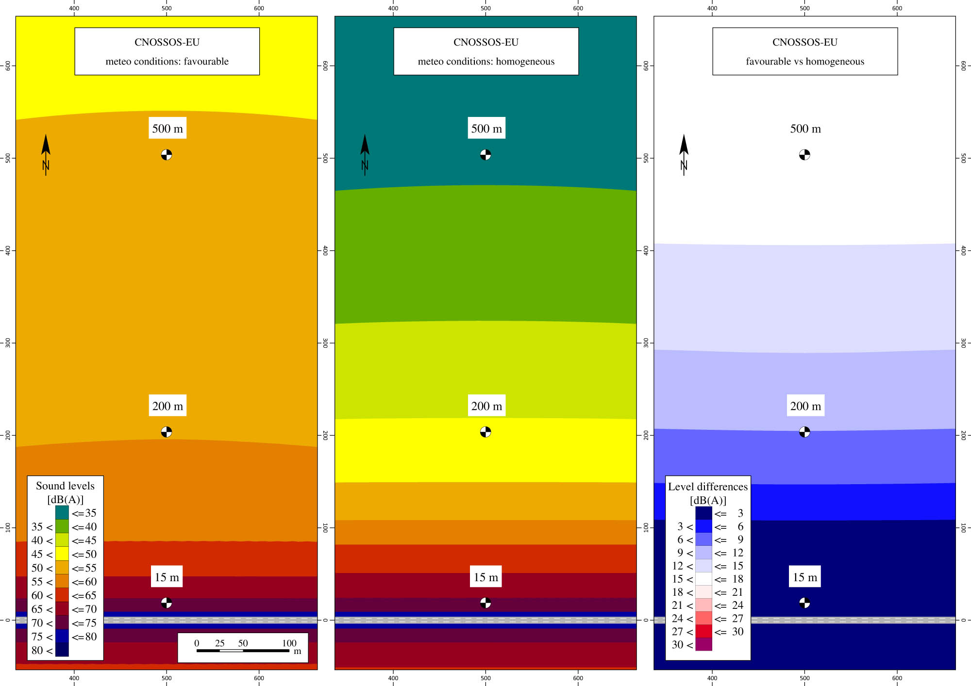
CNOSSOS-EU sound level grid maps with soft ground (G = 0.8). Left: favourable conditions; centre: homogeneous conditions; right: sound level differences.

NORD2000 parametric sound level grid maps with soft ground (G = 0.8). Left: favourable conditions; centre: unfavourable conditions; right: sound level differences.

NORD2000 statistical sound level grid maps with soft ground (G = 0.8). Left: favourable conditions; centre: unfavourable conditions; right: sound level differences.
5 Discussion
Under favourable sound propagation conditions, all methods provide similar results for hard and soft ground.
Under homogeneous/unfavourable sound propagation conditions, differences in results are nearly negligible between NMPB and CNOSSOS-EU for hard ground, with a maximum value of 2.5 dB at receiver R3, whereas, for soft ground, differences are 5.8 and 7.8 dB at receivers R2 and R3, respectively. Large differences in sound levels, ranging from 6.2 dB (R3, G = 0.8) to 8.2 dB (R2, G = 0.2), also occur between NORD2000 parametric and NORD2000 statistical. Very large differences have been observed between NMPB or CNOSSOS-EU on the one hand and NORD2000 parametric or statistical on the other. In particular:
for hard ground, sound level differences range from 8.4 dB (receiver R2, CNOSSOS-EU vs NORD2000 parametric) to 25.1 dB (receiver R3, NMPB vs NORD2000 statistical);
for soft ground, sound level differences range from 14.4 dB (receiver R2, CNOSSOS-EU vs NORD2000 parametric) to 32.9 dB (receiver R3, NMPB vs NORD2000 statistical).
NMPB shows sound level differences between favourable and homogeneous conditions ranging from 2.1 dB (receiver R2) for hard ground to 10.0 dB (receiver R3) for soft ground. Similarly, results obtained by CNOSSOS-EU show sound-level differences from 3.2 dB (receiver R2) for hard ground to 16.7 dB (receiver R3) for soft ground.
NORD2000 parametric sound-level differences range from 6.4 dB (receiver R2) for hard ground to 34.9 dB (receiver R3) for soft ground, while NORD2000 statistical yields sound-level differences from 17.7 dB (receiver R2) for hard ground to 43.0 dB (receiver R3) for soft ground.
The above differences are due to the features of NORD2000, which reproduces upward-sound-waves refraction (unfavourable sound propagation conditions) differently from what both NMPB and CNOSSOS-EU do as they account only for straight-line sound propagation (homogeneous conditions). Hence, NORD2000 can perform calculations for short-term (30/60 minutes) actual weather conditions, whereas the other two methods provide results only for long-term (some months or one-year) average weather conditions.
For favourable conditions, sound levels by NORD2000 parametric are lower than those by NORD2000 statistical; on the contrary, they are higher for unfavourable conditions. This outcome is expected because the state of the atmosphere described with the parametric approach is less extreme than that by the statistical one:
the unfavourable condition scenario outlined by the statistical approach with the second (out of 25) meteorological class assumes a ratio D/R cur = −0.23 (D = source-receiver distance, R cur = sound-ray curvature); the parametric calculations, instead, are carried out assuming a diurnal situation with clear sky and a wind speed of 3.0 m/s @ 10 m in the receiver-source direction (180°), approximately corresponding to a D/R cur ratio = −0.10;
the favourable condition scenario outlined by the statistical approach with the 24th (out of 25) meteorological class assumes a ratio D/R cur = 0.23; the parametric calculations, instead, are performed assuming a partly overcast night sky with thermal inversion (no gusts/turbulence) and wind speed of 1.2 m/s @10 m in the source-receiver direction (0°), approximately corresponding to a D/R cur ratio = 0.17.
For homogeneous/unfavourable propagation conditions, the soft ground scenario yields sound-level differences larger than those obtained for the hard ground setting.
Looking at the grid maps for soft ground in Figure 9, the comparison of CNOSSOS-EU (homogeneous) to NORD2000 parametric (unfavourable) shows that: i) from about 50 m from the source to longer distances, the sound-level difference exceeds 3 dB; ii) at 100 m distance from the source, the sound level difference ranges from 12 to 15 dB.
Referring to Figures 10–13, the distance from the source at which the sound-level difference between favourable and homogeneous/unfavourable conditions exceeds 3 dB is as follows:
about 80 m for NMPB;
about 110 m for CNOSSOS-EU;
about 45 m for NORD2000 parametric;
about 20 m for NORD2000 statistical.
The calculations by NORD2000 parametric (Figure 12) are consistent with formula 11 in paragraph 8.1, page 12 of ISO 1996-2:2017 [15], stating that, for soft ground, sound-level variations due to meteorological conditions are modest (<3 dB) for a source-receiver distance D ≤ 10 × (hs + hr), where hs = source height and hr = receiver height. This formula also shows that meteorological conditions and ground effects are less influencing the propagation for taller sources and receivers, as can be seen from the cross section in Figure 14 (the cross section set for NORD2000 can be found in the supplementary material, Figures S11 and S12).

NORD2000 parametric sound-level cross sections for soft ground (G = 0.8). From top: favourable conditions, unfavourable conditions, favourable vs unfavourable level differences, level differences zoom.
Also, calculations with NORD2000 parametric were carried out considering a point source with the same sound power spectrum, sound pressure level at R1, distance from the receivers, and height as the straight road. The results in Table 6 show the same trend for both sources, with the point source slightly deemphasising the effects of changing weather conditions (and ground absorption). In the supplementary material, grid maps (G = 0.8) and cross sections (G = 0.2 and 0.8) can be found in Figures S13 and S14, respectively.
Level differences (dB) (favourable–unfavourable) conditions for NORD2000 parametric for different sources
| Receiver | Ground absorption G | Road source | Point source |
|---|---|---|---|
| R1 (15 m) | 0.2 | 0.1 | 0.1 |
| 0.8 | 0.5 | 0.0 | |
| R2 (200 m) | 0.2 | 6.4 | 3.8 |
| 0.8 | 24.8 | 17.4 | |
| R3 (500 m) | 0.2 | 16.8 | 14.1 |
| 0.8 | 34.9 | 28.1 |
6 Conclusions
Under favourable propagation conditions, differences of up to 5.6 dB at 500 m source-receiver distance with hard ground show up (between CNOSSOS-EU and NORD2000 parametric), but all the considered calculation methods perform similarly, as expected.
Only the NORD2000 method can account for unfavourable conditions, and sound-level differences between favourable and unfavourable conditions reach a maximum of 27.3 dB for hard ground and 43.0 dB for soft ground at a source-receiver distance of 500 m.
Homogeneous conditions cannot be a surrogate, not to say a substitute, for unfavourable conditions since the level differences between unfavourable NORD2000 statistical and homogeneous NMPB-Routes 1996 conditions are as high as 25.1 dB for hard ground and 32.9 dB for soft ground; also, at 500 m source-receiver distance, the smaller level difference is 14.7 dB (with hard ground) between the unfavourable NORD2000 parametric and the homogeneous CNOSSOS-EU conditions.
The above considerations are crucial when planning and performing long-range, short-term sound level measurements either for fine-tuning acoustic models in the set-up phase or for running post-completion tests.
For practical reasons, such measurements are often performed during the day. However, as pointed out in the study by Wilson [28], refractive effects are never negligible for all propagation directions, regardless of atmospheric conditions; downward refraction rarely occurs during the day, even in the downwind direction, except when the wind speed is more than about 5 m/s, and there is cloud cover. Therefore, the engineering calculation method used for the simulation must be able to reproduce all propagation conditions.
Some rules of thumb can help when planning measurement campaigns:
in windy weather, regardless of the period of the day, the temperature stratification is almost neutral; the refraction, downward or upward, depends on the wind propagation direction;
with low wind and clear sky during the day time, the atmosphere is unstable and turbulent due to warm air rising from the ground; in such conditions, upward refraction is expected;
with low wind and cloudy sky, regardless of the period of the day, weak turbulence and upward refraction are present in all directions;
with low wind and clear sky during the night, the atmosphere is stable, and downward refraction is present, enhanced when thermal inversion occurs.
However, regardless of the typical situations outlined above, the ABL is a complex system continuously varying in time and space. The concepts and analyses herewith given show that knowledge of the basic principles of meteorology and the calculation methods’ capability of reproducing distinct weather conditions, on the one hand, and technical skills and tools, on the other hand, are required to obtain meaningful information from data about atmospheric stability besides wind speed and direction, relative humidity, and temperature.
Acknowledgements
Section 2 of the article is particularly inspired by Roland B. Stull’s “Practical Meteorology: an Algebra-Based Survey of Atmospheric Science” (the study by Stull [9]).
-
Funding information: The authors state no funding involved.
-
Author contributions: All authors accepted the responsibility for the content of the manuscript and consented to its submission, reviewed all the results, and approved the final version of the manuscript. AT (Andrea Tombolato) and GB were responsible for the overall supervision of the project. AT (Andrea Tombolato) and AT (Alberto Troccoli) were involved in writing the second section entitled “Practical Meteorology.” AT (Andrea Tombolato), FB, and AS were responsible for model design and calculations. AT (Andrea Tombolato), GB, and FB were responsible for the conclusions.
-
Conflict of interest: Authors A.T. (Andrea Tombolato) and F.B. are employees of Acusticapd. Author A.S. is a noise consultant. The authors declare no other conflict of interest.
-
Supplementary material: In the supplementary material, grid maps and cross sections are provided as cited in the text.
References
[1] Embleton TFW. Tutorial on sound propagation outdoors. J Acoust Soc Am. 1996;100:31–48.10.1121/1.415879Search in Google Scholar
[2] Attenborough K, Bass HE, Di X, Raspet R, Becker GR, Güdesen A, et al. Benchmark cases for outdoor sound propagation models. J Acoust Soc Am. 1995;97:173–91.10.1121/1.412302Search in Google Scholar
[3] Salomons EM. Computational atmospheric acoustics. Dordrecht: Kluwer; 2002.10.1007/978-94-010-0660-6Search in Google Scholar
[4] Bérengier MC, Gavreau B, Blanc-Benon P, Juvé D. A short review of recent progress in modelling outdoor sound propagation. Acta Acust U Acust. 2003;89:980–91.Search in Google Scholar
[5] Attenborough K, Van Renterghem T. Predicting outdoor sound. 2nd edn. Boca Raton: CRC Press, Taylor & Francis Group; 2021.10.1201/9780429470806Search in Google Scholar
[6] International Organization for Standardization. ISO 2533:1975. Standard atmosphere. Geneva: ISO; 1975.Search in Google Scholar
[7] NOAA. NOAA-S/T 76-1526. U.S. Standard Atmosphere, 1976. Washington, DC: U.S. Gov. Print. Off.; 1976.Search in Google Scholar
[8] Cavcar M. The International Standard Atmosphere (ISA). Vol. 30, Eskişehir, Turkey: Anadolu University; 2000.Search in Google Scholar
[9] Stull R. Practical Meteorology: An Algebra-based Survey of Atmospheric Science-version 1.02b. Univ. of British Columbia; 2017. https://www.eoas.ubc.ca/books/Practical_Meteorology/.Search in Google Scholar
[10] Sathe A, Mann J, Gottschall L, Courtney M. Estimating the systematic errors in turbulence sensed by wind lidars. Risø National Laboratory, Roskilde, Denmark: Risø; 2022.Search in Google Scholar
[11] Piercy JE, Embleton TWF, Sutherland LC. Review of noise propagation in the atmosphere. J Acoust Soc Am. 1977;61:1403–18.10.1121/1.381455Search in Google Scholar PubMed
[12] Sutherland LC, Daigle GA. Atmospheric sound propagation. In: Crocker MJ, editor. Encyclopedia of acoustics. New York: Wiley; 1997. p. 341–65.10.1002/9780470172513.ch32Search in Google Scholar
[13] Heimann D, Salomons EM. Testing meteorological classifications for the prediction of long-term average sound levels. Appl Acoust. 2004;65:925–50.10.1016/j.apacoust.2004.05.001Search in Google Scholar
[14] Wilson DK, Pettit CL, Ostashev VE. Sound propagation in the atmospheric boundary layer. Melville, NY: Acoustical Society of America; 2015.Search in Google Scholar
[15] International Organization for Standardization. ISO 1996-2:2017. Acoustics. Description, measurement and assessment of environmental noise. Part 2: determination of sound pressure levels. Geneva: ISO; 2017.Search in Google Scholar
[16] Directive 2002/49/EC of the European Parliament and the Council of 25 June 2002 relating to the assessment and management of environmental noise. Official Journal of the European Communities. 2002;L189(vol. 45):12–25.Search in Google Scholar
[17] International Organization for Standardization. ISO 9613-1:1993. Acoustics. Attenuation of sound during propagation outdoors. Part 1: calculation of the absorption of sound by the atmosphere. Geneva: ISO; 1993.Search in Google Scholar
[18] Dutilleux G, Defrance J, Gauvreau B, Besnard F. The revision of the French method for road traffic noise prediction. J Acoust Soc Am. 2008;123(5):3150. 10.1121/1.2933163.Search in Google Scholar
[19] Commission Directive (EU) 2015/996 of 19 May 2015 establishing common noise assessment methods according to directive 2002/49/EC of the European Parliament and of the Council. Official Journal of the European Union. 2015;L168(vol. 58):1–823.Search in Google Scholar
[20] Fredianelli L, Licitra G, Dutilleux G, Cueto L. Industrial and transport infrastructure noise. In: Physical Agents in the Environment and Workplace: Noise and Vibrations, Electromagnetic Fields and Ionizing Radiation. Boca Raton: CRC Press, Taylor & Francis Group; 2018.10.1201/b22231-2Search in Google Scholar
[21] Maijala P, Kontkanen O. CNOSSOS-EU sensitivity to meteorological and to some road initial value changes. In: INTER-NOISE and NOISE-CON Congress and Conference Proceedings. Institute of Noise Control Engineering. Vol. 253. Issue 2; 2016. p. 6245–56.Search in Google Scholar
[22] Khan J, Ketzel M, Jensen SS, Gulliver J, Thysell E, Hertel O. Comparison of Road Traffic Noise prediction models: CNOSSOS-EU, Nord2000 and TRANEX. Environ Pollut. 2021;270:116240. 10.1016/j.envpol.2020.116240.Search in Google Scholar PubMed
[23] Kragh J, Jonasson H, Plovsing B, Sarinen A. User’s guide Nord2000 road; 2006. https://www.studocu.com/da/document/danmarks-tekniske-universitet/trafik-og-veje-i-byomrader/users-guide-nord2000-road/27816530.Search in Google Scholar
[24] Plovsing B, Kragh J. Nord2000. Comprehensive Outdoor Sound Propagation Model. Part 1: Propagation in an Atmosphere without Significant Refracion. DELTA Acoustics & Vibration Revised Report AV 1849/00; 2006.Search in Google Scholar
[25] Plovsing B, Kragh J. Nord2000. Comprehensive Outdoor Sound Propagation Model. Part 2: Propagation in an Atmosphere with Refracion. DELTA Acoustics & Vibration Revised Report AV 1851/00; 2006.Search in Google Scholar
[26] Eurasto R. Nord2000 for Road Traffic Noise Prediction. WP4: Weather Classes and Statistics. VTT Report VTT-R-02530-06; 2006.Search in Google Scholar
[27] Kragh J. Traffic noise prediction with Nord2000-an update. In: Proceedings of Acoustics; 2011.Search in Google Scholar
[28] Wilson DK. The sound-speed gradient and refraction in the near-ground atmosphere. J Acoust Soc Am. 2003;113(2):750–7. 10.1121/1.1532028.Search in Google Scholar PubMed
© 2024 the author(s), published by De Gruyter
This work is licensed under the Creative Commons Attribution 4.0 International License.
Articles in the same Issue
- Regular Articles
- Low-frequency cabin noise of rapid transit trains
- Utilizing the phenomenon of diffraction for noise protection of roadside objects
- Benchmarking the aircraft noise mapping package developed for a unified urban environmental modelling tool
- Acoustical analysis and optimization design of the hair dryers
- Methodologies for the prediction of future aircraft noise level
- Basics of meteorology for outdoor sound propagation and related modelling issues
- Predictive noise annoyance and noise-induced health effects models for road traffic noise in NCT of Delhi, India
- Modeling and mapping of traffic noise pollution by ArcGIS and TNM2.5 techniques
- A novel method for constructing large-scale industrial noise maps based on open source data
- Understanding perceived tranquillity in urban Woonerf streets: case studies in two Dutch cities
- Review Article
- A comprehensive review of noise pollution monitoring studies at bus transit terminals
- Rapid Communication
- The Environment (Air Quality and Soundscapes) (Wales) Act 2024
- Erratum
- Erratum to “Comparing pre- and post-pandemic greenhouse gas and noise emissions from road traffic in Rome (Italy): a multi-step approach”
- Special Issue: Latest Advances in Soundscape - Part II
- Soundscape maps of pleasantness in a university campus by crowd-sourced measurements interpolation
- Conscious walk assessment for the joint evaluation of the soundscape, air quality, biodiversity, and comfort in Barcelona
- A framework to characterize and classify soundscape design practices based on grounded theory
- Perceived quality of a nighttime hospital soundscape
- Relating 2D isovists to audiovisual assessments of two urban spaces in a neighbourhood
- Special Issue: Strategic noise mapping in the CNOSSOS-EU era - Part I
- Analysis of road traffic noise in an urban area in Croatia using different noise prediction models
- Citizens’ exposure to predominant noise sources in agglomerations