Benchmarking the aircraft noise mapping package developed for a unified urban environmental modelling tool
-
Linus Yinn Leng Ang
 ,
Fangsen Cui
,
Fangsen Cui

Abstract
In densely populated cities, residents living near aerodromes may experience heightened exposure to aircraft noise. With hybrid work arrangement, authorities have observed a rise in the number of complaints filed by residents affected by aircraft noise. In view of this problem, urban planners are now placing even more emphasis on exploring solutions that can manage aircraft noise in new and existing residential areas. To achieve this objective, urban planners usually rely on external acoustic consultants to generate noise maps using commercial software. However, urban planners may need to quickly evaluate potential noise issues in the neighbourhood so that noise management strategies can be brainstormed in advance. In this article, we present the development and benchmarking of a package designed to easily generate aircraft noise maps via simplified procedures and a reduced amount of input data, with acceptable accuracy in the results. These benefits distinguish our developed package from commercial software. Our developed package was eventually integrated into an in-house-developed unified urban environmental modelling tool that aims to help urban planners design more liveable and sustainable residential towns in an intuitive and quick manner.
1 Introduction
The recent emphasis on building sustainable and smart cities has driven advancements and innovative approaches related to noise mapping, a crucial domain within environmental acoustics [1–3]. While environmental noise encompasses a range of sources including road traffic, aircraft, and railways, research has predominantly concentrated on managing road traffic noise. Cutting-edge technologies such as advanced real-time evaluation techniques [4,5] and the application of artificial intelligence [6–8] have revolutionised noise mapping methodologies, allowing for more accurate and comprehensive assessments. Enhanced monitoring stations equipped with sophisticated sensors enable precise data collection, facilitating detailed analyses of noise distribution patterns and trends [9,10]. Recent attention has been directed towards electric vehicle transportation [11–13] and low-noise pavements [14,15], acknowledging their potential contributions to reducing overall urban noise pollution.
Many organisations have formally retained hybrid work arrangement to provide employees with flexibility [16]. For example, eligible employees are encouraged to work in the office for at least 3 days per week. For the remaining days, they are given the option to work remotely. Some organisations believe that remote work can help boost productivity among employees because less time is spent on getting ready and commuting [17]. In addition, formalising hybrid work arrangement can be seen as an opportunity for organisations to cut down on rental expenditures because less office space is needed. As more organisations formally include hybrid work arrangement in their policies, the stay-home population during office hours is expected to be large.
Following the ease of cross-border travel restrictions, air traffic is picking up to pre-pandemic levels. Although this improving situation is a good sign of economic recovery, the built environment is again polluted with aircraft noise like how it was before the pandemic. In the past, air traffic was already high, but employees rarely had the option to work remotely. With hybrid work arrangement, authorities have observed a rise in the number of complaints filed by residents due to aircraft noise. Despite the many modes of transport that contribute to noise pollution, research has shown that aircraft noise plays a significant role in determining how annoying the noise pollution is.
For example, Wothge et al. [18] surveyed more than 9,500 residents around Frankfurt Airport (Germany) in 2017 to study the influence of aircraft noise combined with another transportation noise – either railway or road traffic – on annoyance. The findings showed that residents would feel annoyed whenever aircraft noise dominated the other transportation noise. In Switzerland, Schäffer et al. [19] surveyed more than 5,500 residents in 2020 to study the impact of green spaces on annoyance resulting from road traffic noise, railway noise, and aircraft noise. The survey found that with more green spaces, residents would feel less annoyed by railway noise and road traffic noise. However, for aircraft noise, residents continued to feel annoyed despite having more green spaces. In 2019, the World Health Organisation published the environmental noise guidelines for the European region [20], offering evidence-based conclusions that, at equivalent noise levels, aircraft noise induces greater annoyance compared to road traffic and railway noise.
Although aircraft noise is the leading contributor of annoyance among residents, evidence remains lacking in proving how chronic aircraft noise exposure can afflict mental health [21]. Nevertheless, research has firmly established that chronic exposure to aircraft noise can indirectly lead to health issues, such as cognitive impairment in children and cardiovascular disease [22]. In 2019, Sparrow et al. [23] highlighted that studies have discovered compelling evidence linking exposure to aircraft noise with cognitive impairment in children, particularly affecting their reading comprehension. Separately, in 2014, Babisch [24] reported that most studies consistently found evidence suggesting an increased risk of developing cardiovascular disease with higher noise levels. To aid understanding, a flow diagram illustrating the simplified chain reactions between transportation noise exposure and cardiovascular disease was created. Other than health issues, aircraft noise is known to affect housing prices as well [25,26]. Evidently, with hybrid work arrangement, managing aircraft noise can help improve the work environment for the stay-home population during office hours.
As residents, closing the windows during office hours is the most straightforward way to minimise aircraft noise from entering the living space. If soundproof windows are installed, further noise reduction can be achieved [27]. In view of exterior aesthetics, some property developers may prohibit residents from changing the windows. Although residents can enjoy better indoor acoustic comfort after closing the windows, productivity may not increase owing to the lack of natural ventilation. Unless air conditioning is present, poor indoor thermal comfort can also adversely affect productivity [28]. Considering the growing interest in developing sustainable cities to combat climate change, natural ventilation is preferred over mechanical ventilation for energy conservation.
As small cities grow denser in population, the demand for residential buildings will naturally rise. Land scarcity may result in the development of residential buildings nearer to a busy airdrome. Instead, an existing airdrome may be redesigned and relocated elsewhere that is surrounded by residential buildings. Either way, residents may find difficulty maintaining concentration at work, affecting productivity. For urban planners, they must evaluate the potential repercussions resulting from the changes and collaborate closely with relevant authorities to effectively manage aircraft noise [29–33]. In Asia, the Kaohsiung International Airport (Taiwan) [34], the Gimpo International Airport (South Korea) [35], the Tengah Air Base (Singapore) [36], the Changi International Airport (Singapore) [37], and the Hangzhou Xiaoshan International Airport (China) [38] are examples with residential buildings found nearby.
Seeing how hybrid work arrangement has become a formal norm in more organisations, urban planners are now placing even more emphasis on exploring solutions that can manage aircraft noise in new and existing residential areas. To ensure efficient resource management, it is imperative to identify problematic regions in the neighbourhood before brainstorming for solutions. For existing neighbourhoods, residents can be engaged through surveys to garner their feedback. For example, in 2023, the Federal Aviation Administration [39] updated the National Sleep Study database with the latest survey findings. Residents who participated (400) were surveyed for 2 years to study the effects of nocturnal aircraft noise on their sleep. The findings helped inform authorities about the need for potential revisions to existing noise regulations. For new neighbourhoods under development, noise maps can be used. For assurance, site visits can also be conducted because there may be other physical factors present on-site – preserved infrastructures, for example – that affect the accuracy of the noise maps. Heinonen-Guzejev et al. [40] showed that noise maps are also applicable for existing neighbourhoods and can be used to validate survey findings.
A noise map is a form of data visualisation that provides urban planners with insights into the intensity and distribution of noise in a neighbourhood. To compute accurate noise maps, commercial software requires the user to define a plethora of input parameters. In most cases, some input parameters are unknown. As such, the user is required to complete the scenario by making informed assumptions, which may or may not affect the accuracy of the noise map. Also, because commercial software performs most computations in a black box, it is difficult to fully comprehend the assumptions made [41]. Considering that urban planners are mostly not specialised in acoustics, defining every input parameter can be a challenging task, not to mention time-consuming. Instead, urban planners rely on acoustic consultants to provide accurate noise maps. As acoustic consultants are often handling multiple projects, it may take a few weeks before urban planners receive the noise maps. Occasionally, while waiting, urban planners may need to quickly evaluate potential noise issues in the neighbourhood so that noise management strategies can be brainstormed in advance. Therefore, there is a need for urban planners to possess a simulation tool that does not have a steep learning curve and is able to easily produce noise maps based on the specific needs of local regulations.
Although not specifically developed with urban planners in mind, researchers have recognised the need for a simulation tool that offers more transparency and flexibility in producing noise maps resulting from aircraft operations. A notable example is the model (sonAIR) developed by the Swiss Federal Laboratories for Materials Science and Technology (Empa) [42–44]. The motivation behind the development stemmed from the necessity to generate noise maps arising from novel aircraft designs or updated flight procedures without the need for input data, such as the geometry of aircraft components, which may not be readily available.
In another example, Riboldi et al. [45] saw the need to develop a model that can produce noise maps resulting from new battery-powered aircraft designs. The model was developed based on ECAC Doc 29 [46–48]. Established by the European Civil Aviation Conference (ECAC), ECAC Doc 29 is widely regarded as one of the best practice models for producing noise maps resulting from aircraft operations. The Environmental Noise Directive published by the European Union [49] also recommends the utilisation of ECAC Doc 29. Based on the same best practice model, others have also implemented computation procedures to consider non-towered airports [50] and ground operations [51].
In our case, we have been internally developing a unified urban environmental modelling tool [52] that aims to help urban planners design more liveable and sustainable residential towns in an intuitive and quick manner. Setting itself apart from commercial software, the modelling tool has the capability to seamlessly integrate a range of environmental factors, including wind flow, solar exposure, wind-driven rain, building energy usage, and outdoor noise. As a result, it can analyse the interdependencies and cumulative effects of these environmental factors on a given urban setting.
As discussed in earlier paragraphs, the rising demand for hybrid work arrangement and the steep learning curve of commercial software motivated us to include aircraft noise mapping as one of the features in the modelling tool. While commercial software can offer great flexibility in scenario creation, urban planners can benefit from automated processes to quickly evaluate potential noise issues in the neighbourhood so that noise management strategies can be brainstormed in advance. Based on ECAC Doc 29, we developed the package such that noise maps can be easily generated via simplified procedures and a reduced amount of input data, with acceptable accuracy in the results. These benefits distinguish our developed package from commercial software. However, we must stress that the results produced by our developed package are intended primarily for quick evaluation and should be regarded as approximate. Ultimately, it is advisable to validate the results through field measurement data and benchmarking with commercial software tailored for comprehensive noise calculations. This article aims to present how the aircraft noise mapping package was developed and benchmarked.
This article is structured in a sequential manner. Each section builds upon the previous one to provide a logical understanding of the whole research and development process. In Section 2, we present the development of the aircraft noise mapping package by discussing the methodology, algorithms, and data sources employed. Next, in Section 3, we present how the results were benchmarked against those obtained from the commercial software, SoundPLAN. Before concluding this article in Section 5, we discuss the main limitations of our developed package and the potential avenues for consideration as future work in Section 4.
2 Development of the aircraft noise mapping package
The aircraft noise mapping package consists of algorithms fully written in Python. Essential libraries include NumPy, pandas, SymPy, Matplotlib, and imageio. This section describes how the package was developed in the back-end (Sections 2.1–2.3) and presented in the graphical user interface (GUI) (Section 2.4).
2.1 Selecting the reference model
Aircraft noise prediction models can be classified into theoretical (or scientific) models and best practice models. Theoretical models are designed to estimate the absolute noise level of an aircraft that does not currently exist, accounting for unconventional configurations, new designs, or novel operating procedures. However, due to their proprietary nature, theoretical models may have limited accessibility for widespread use. Conversely, best practice models offer a more practical and user-friendly approach, making them suitable for users without extensive technical expertise. Best practice models prioritise providing users with a quick understanding of the noise distribution across a specific land area. It is worth noting that best practice models rely exclusively on measurements published by manufacturers, limiting their analysis to existing aircraft. Ang and Cui [22] recently published a review article that offers a more detailed background relating to this topic.
As summarised by Ang and Cui [22], notable examples of aircraft noise prediction models include DLR AzB, ECAC Doc 29, and ICAO Doc 9911. These models were developed by the German Aerospace Centre (DLR), the ECAC, and the International Civil Aviation Organisation (ICAO), respectively. Among these models, ECAC Doc 29 is widely used because its guidelines were partially incorporated into both DLR AzB and ICAO Doc 9911, serving as the foundation. Pertaining to language, both ICAO Doc 9911 and ECAC Doc 29 are published in English. Pertaining to availability, only ECAC Doc 29 is an open access resource. It relies on the Aircraft Noise and Performance (ANP) database [53], which is also free to access. Considering these factors, we selected ECAC Doc 29 as the reference that guided our development of the aircraft noise mapping package. Although ECAC Doc 29 consists of three volumes [46–48], only the second volume contains the guidelines for algorithm development.
2.2 Selecting the noise metric
There are two categories of noise metrics that quantify aircraft noise. They are single-event and cumulative noise metrics. For single-event noise metrics, commonly used examples include maximum noise level (
Being a new development, the aircraft noise mapping package was designed to consider only single-event flights quantified by one noise metric. Naturally, only single-event noise metrics (
2.3 Designing the algorithm workflow
The aircraft noise mapping package consists of three modules that form the algorithm workflow (Figure 1). These modules were designed to operate sequentially, with the outputs of the first module serving as inputs for the second module and the outputs of the second module serving as inputs for the third module. Fundamentally, the first, second, and third modules fulfil the respective roles of the pre-processor, solver, and post-processor within the package. The following sections are dedicated to presenting the workflow of each module.
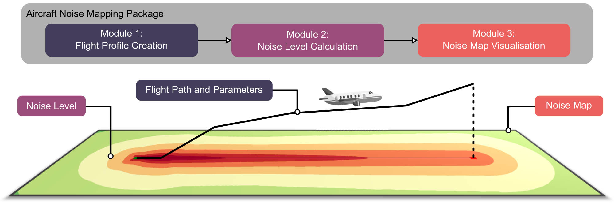
An overview of the aircraft noise mapping package consisting of three modules that form the algorithm workflow.
At this point, it is important to mention that this section does not cover every equation used in the developed package. They are well described in ECAC Doc 29 Vol 2. In this section, only those essential for understanding the algorithm workflow are discussed. It is also important to note that equations and parameters used in aviation are often expressed in imperial units. To be consistent with the literature, including ECAC Doc 29 Vol 2, this section adopts the same units to minimise the use of conversion constants that may otherwise cause unnecessary complications or make the equations appear unfamiliar. Despite this, since the modelling tool employs metric units as its default system of measurement, all results and quantities within the GUI are presented in metric units. Unless otherwise stated, the values of all variables can be obtained from the embedded ANP database.
2.3.1 Module 1: Flight profile creation
In the GUI, the user starts by selecting the aircraft of interest and specifying the flight type (departure or arrival) for the simulation. Although the ANP database provides datasets for more than 100 aircraft models, only 30 of them were integrated into the module. The datasets provide all modules with the essential information needed to compute the noise maps. The information includes the general specifications, engine coefficients, aerodynamic coefficients, flight procedures, and noise-power-distance (NPD) values of the aircraft.
Other than aircraft and flight type, the user may edit the default values of the parameters that define the reference condition of the aerodrome. The parameters include ambient air pressure, ambient air temperature, headwind, runway elevation, runway gradient, and runway length. The values of the first two parameters are given based on the International Standard Atmosphere at mean sea-level [54]. The values of the next three parameters are given based on those published by the manufacturers when they measured the engine coefficients [47]. In reality, wind conditions are rarely constant and can vary widely. For the sake of simplicity, ECAC Doc 29 Vol 2 recommends keeping the wind speed and direction constant regardless of altitude. If needed, the user can define a tailwind by entering a negative wind speed. The module will recognise the entry as a tailwind. Considering that the modelling tool will be largely used to study scenarios within Singapore, the default runway length is given as the length of the runways at Changi International Airport, which is the main airport of Singapore. This information reduces the time spent on literature search for the user. Finally, the default runway heading is provided based on the scenario in which the aircraft is departing eastward or arriving from the west. The runway heading is positive when specified clockwise from the magnetic north. A summary of the default values is shown in Table A1.
The back-end algorithm reads the user-input values and executes the relevant computations (Figure 2) to output the flight profile. The flight profile contains the flight path segmented according to the guidelines in ECAC Doc 29 Vol 2. Every segment is defined by one starting point (
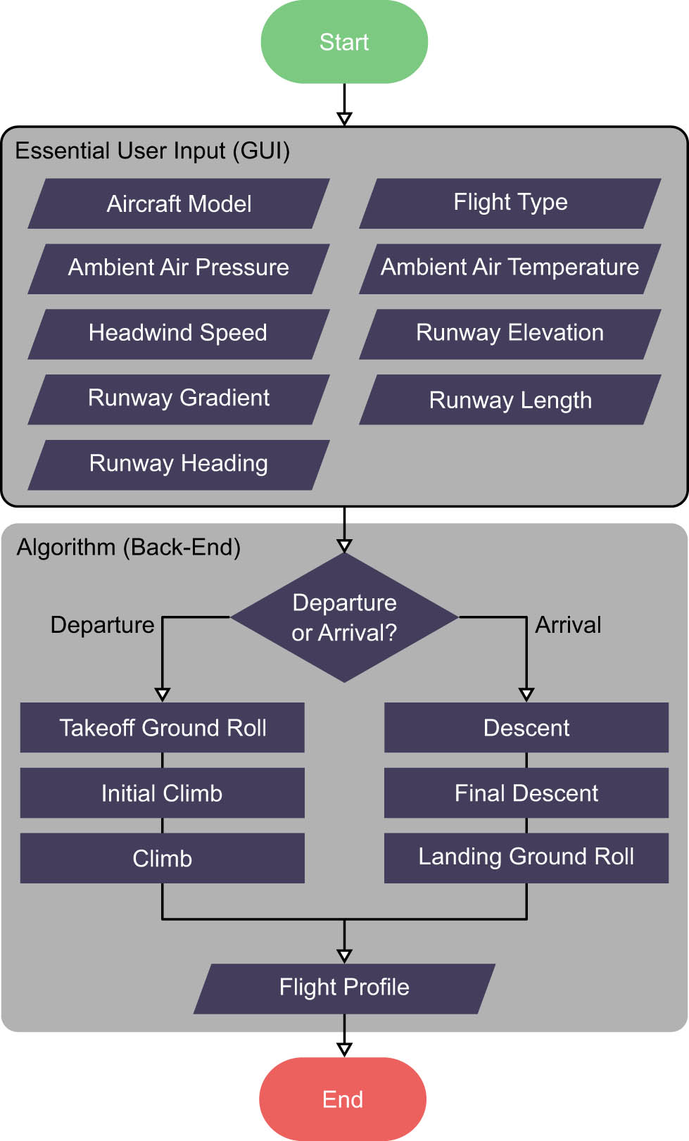
Flowchart of Module 1. The output (flight profile) contains the flight path segments, each defined by one starting point (
2.3.1.1 Takeoff ground roll
For departure, the first step (Tables A2 and A4) is to compute the flight profile when the aircraft is on the runway, which is between the brake release point and the takeoff point. In practice, it is common for the aircraft to stop completely at the brake release point and wait for takeoff clearance. As such, the module will always assign 0 kt to the initial CAS of the step. At the takeoff point, the CAS is approximated using
where
where
The length of the flight path is described by the ground distance covered. Specific to the takeoff ground roll, the following equation is used:
where
where
The module proceeds to compute the performance parameters (CAS and CNT) for every segment. ECAC Doc 29 Vol 2 specifies that the performance parameters are assumed to increase linearly from one segment to another during the takeoff ground roll. As the initial and final CAS of the step are already known (equation (2)), the module only needs to compute the change in CAS per segment using the following equation:
where the same applies for the change in CNT per segment, replacing
The approach to computing the CNT for one engine type may not apply for another engine type. The module can support turboprop, turbojet, and turbofan engines, which are the common engine types found in local aerodromes. For turboprop engines, the CNT is computed using
where
where
2.3.1.2 Initial climb
Once the aircraft is airborne, the module computes the flight profile specific to the initial climb, which extends from the takeoff point to the point where the altitude is 1,000 ft (Tables A2 and A4). Here, the aircraft operates at a constant speed. Therefore, the module assigns the final CAS the same value of the initial CAS (i.e.,
Unlike the takeoff ground roll, the approach to segmenting the flight path of the initial climb is based on a list of reference altitudes given in ECAC Doc 29 Vol 2. Established from past research, the approach was shown to produce reliable noise predictions when the aircraft is close to the ground. In this way, the change in lateral attenuation per segment is kept within 1.5 dB. Knowing the initial and final altitudes of every segment and the number of segments, the ground distance covered per segment is estimated using
where
where
2.3.1.3 Climb
For the rest of the climb, the aircraft accelerates from time to time until the maximum allowable speed is attained. After which, the aircraft maintains the same speed until it reaches 10,000 ft in altitude – the highest point of interest for noise predictions. The module determines if the aircraft is accelerating or not from the flight procedures (Tables A2 and A4).
If the step involves acceleration, the module will check whether there is a change in thrust rating from the previous step. If the check returns true, the module will implement a transition step for thrust cutback immediately after the previous step. Examples are given by the fourth step in Table A2 and the third step in Table A4. In practice, implementing thrust cutback can help extend engine life and reduce noise pollution. The guideline [47] specifies that the transition step should take place over a ground distance of 1,000 ft. For the sake of simplicity, the aircraft is assumed to operate at a constant speed. Hence, segmenting the flight path is not needed. The cutback CNT is computed using
where
If the check returns false, the module will enter an iterative loop designed to determine the final altitude of the step. Examples are given by the sixth step in Tables A2 and A4. In the first iteration, the final altitude is estimated by adding 250 ft to the initial altitude, as specified in ECAC Doc 29 Vol 2. Using this initial estimate, the objective is to re-estimate the final altitude from the flight path and the performance parameters computed using
where
where
In equations (11) and (12), the climb gradient is approximated using
where ROC (ft/min) denotes the rate of climb. To end the iterative loop, the absolute difference between the initial estimate and the re-estimated final altitude (equation (11)) must be within 3 ft. If this condition is not met, the module will begin a new iteration by adding 3 ft to the initial estimate. It is stated in ECAC Doc 29 Vol 2 that the value to use depends on the decision of the developer in striking a balance between accuracy and computational speed. In our case, we decided on 3 ft because it corresponds to about 1 m. For every iteration, the initial estimate is obtained from
where
where
Finally, if the step involves no acceleration, the module will use equations (8) and (9) to compute the flight path and either equation (6) or equation (7) to compute the initial and final CNT where applicable. As the CAS stays the same throughout the step, segmenting the flight path is not required. Examples are given by the fifth step in Tables A2 and A4.
2.3.1.4 Descent
For arrival, noise predictions are concerned with the altitude of 6,000 ft and below. The aircraft must decelerate to the required CAS by the time it enters the final descent at 1,000 ft. Deceleration can take place during either descending or level flight. Examples are given by those before the fourth step in Table A3 and those before the sixth step in Table A5.
If the step requires the aircraft to decelerate and descend concurrently, the module will first compute the ground distance covered using equation (8). This output is then substituted into equation (16), along with the initial and final CAS, to determine the ground distance covered per segment. The number of segments is obtained from equation (2). If the step requires the aircraft to decelerate at a constant altitude, covering a certain ground distance, the module will only need to determine the segment count and the ground distance covered per segment. At this point, the coordinates of the flight path segments are obtained.
Finally, the module computes the initial and final CNT of every segment according to the engine type. For turbojet and turbofan engines, equation (7) is used. For turbofan engines, the following equation is used:
where
The initial and final CAS of every segment are determined via linear interpolation.
2.3.1.5 Final descent
At an altitude of 1,000 ft, the aircraft commences its final descent, which ends at the point when the aircraft is above the landing threshold of the runway (i.e., landing threshold point). Examples are given by the fourth step in Table A3 and the sixth step in Table A5. The approach to segmenting the flight path is the same as that for the initial climb, using the list of reference altitudes given in ECAC Doc 29 Vol 2. Using equation (8), the ground distance covered per segment is determined. At this point, the coordinates of the flight path segments are obtained.
As the CAS is kept constant, every segment is assigned the same value at the starting point and the ending point. Regardless of engine type, the initial and final CNT of every segment are computed from equation (9) by having
2.3.1.6 Landing ground roll
In this last part of the arrival, the flight profile is computed from the landing threshold point to the taxiing point (e.g., last three steps in Tables A3 and A5). The taxiing point refers to the instance when the CAS of the aircraft reaches 30 kt. In practice, the aircraft must complete its rapid deceleration to the taxiing speed after covering a certain ground distance (aircraft-specific) from the touchdown point. This distance is also known as the stop distance. In some situations, it is runway-specific. Examples are given by the sixth step in Table A3 and the eighth step in Table A5.
From the landing threshold point to the touchdown point, the ground distance covered and the average descent angle are given in the flight procedures. Using equation (8), the altitude of the aircraft at the landing threshold point can be estimated. During this period, the performance parameters remain unchanged. Therefore, segmenting this part of the flight path is not needed.
After the touchdown point, the aircraft usually relies on thrust reversal to decelerate rapidly over the stop distance. As the process of thrust reversal varies among aircraft, the module adopts the generalised approach as proposed in ECAC Doc 29 Vol 2. At the moment when the aircraft covered 10% of the stopping distance, the CNT is at 20% of the maximum sea-level static thrust. For the remaining 90% of the stop distance, the CNT is gradually reduced from 20 to 10% of the maximum sea-level static thrust. Equation (16) is used to segment the flight path between the touchdown point and the taxiing point. At this point, the coordinates of the flight path segments are obtained. Finally, the module computes the performance parameters at the starting and ending points of every segment via linear interpolation.
2.3.2 Module 2: Noise level calculation
Now that the flight profile (noise source) of the aircraft is known, the second module helps create the horizontal calculation plane defined by a rectangular or square grid of nodes (noise receivers). The purpose of the module is to return the maximum noise level (

Flowchart of Module 2. The output (overall noise level) contains the coordinates (
In the GUI, the user may choose to provide inputs for up to four parameters that the module uses to define the calculation plane. Otherwise, the user can skip the entries by accepting the default values (Table A1). The grid size specifies the lateral distance between the nodes. The smaller the grid size, the higher the sensitivity of the noise map. The altitude specifies the positive vertical distance of the plane relative to the runway. The GUI displays the last parameter (lateral coverage factor or plane corners) based on the chosen plane type (automatic or manual). For the automatic plane type, the user may specify the lateral coverage factor that determines how large the grid is relative to the bounding box of the ground track. This plane type is useful for obtaining an overview of the noise distribution over an area encompassing the flight path. For the manual plane type, the user must specify two sets of coordinates (
In the back-end, the user-input values are used to create the grid of nodes that form the calculation plane. Together with the flight profile (from Module 1), the spatial information of the nodes is passed to a nested loop designed for noise calculations. The nested loop consists of one outer for loop (for each flight segment) and one inner for loop (for each node). In each inner loop, the module must first compute the spatial relationship between the node and the flight segment to determine whether the node is in front of, behind, or alongside the flight segment, and whether the node is facing the left side, right side, or bottom of the flight segment. This information is essential for the module to appropriately correct the NPD value retrieved from the embedded ANP database, leading to the nodal noise level.
Every NPD value corresponds to the noise level measured at the receiver for a given CNT of the aircraft and its direct distance to the receiver. Aircraft manufacturers would perform the measurements using different noise metrics under the reference condition of the aerodrome. Specific to the
where
Before the computational procedure ends, the module returns the overall noise level (
2.3.3 Module 3: Noise map visualisation
Module 3 provides the user with results visualisation in the form of noise maps, which are available in two types (elaborated later). Figure 4 shows the flowchart of the module.
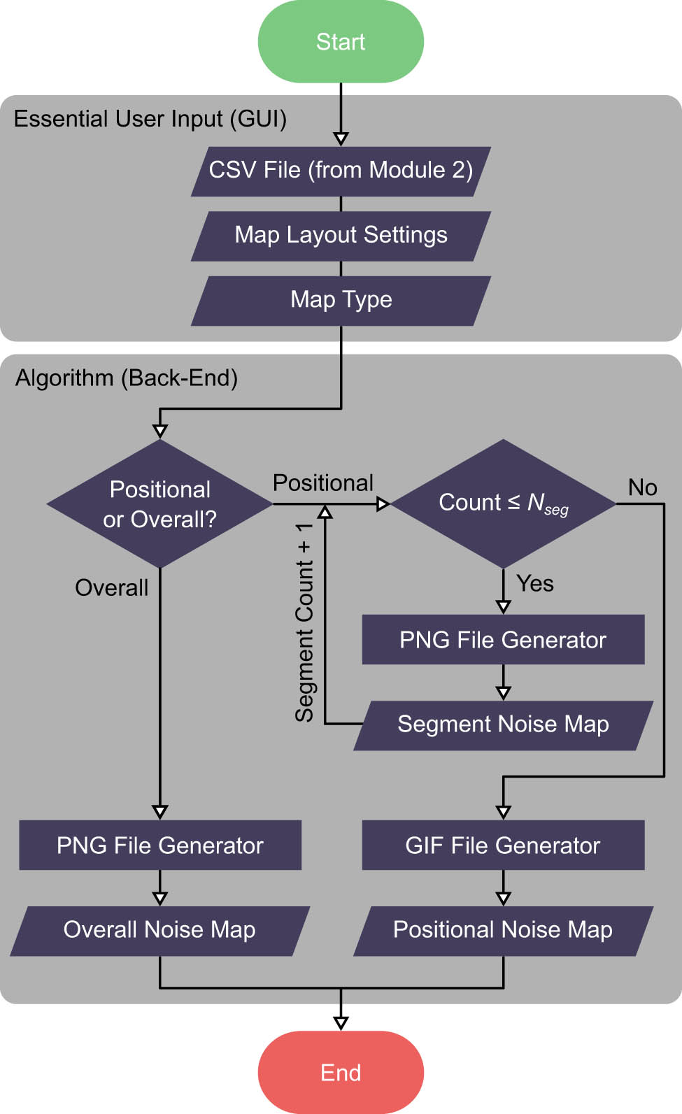
Flowchart of Module 3. All visualisations (overall and positional noise maps) are saved as their respective file formats in the working directory and then displayed in the GUI.
In the GUI, the user must import the results (CSV file from Module 2) so that the back-end has datasets to process into noise maps. The remaining entries are optional to fill. Under map layout settings, the user may specify the contour range, contour interval, and aspect ratio. Additionally, the user may toggle between displaying and hiding the runway and the flight path in the noise map. Otherwise, the user can skip the entries by accepting the default settings. The last entry (map type) is an either/or radio button that the module uses to determine the type of noise map (overall or positional) that should be presented for results visualisation.
In the back-end, the file generators are the core algorithms that process the user-input values and results into noise maps. The overall and positional noise maps are generated as a portable network graphics (PNG) file and a graphics interchange format (GIF) file, respectively. The overall noise map shows the noise distribution (
2.4 Simplifying the GUI workflow
As the GUI was developed by another team (see acknowledgements), it is beyond the scope of this article to discuss the front-end aspects in great detail. Here, the GUI specific to the aircraft noise mapping feature is briefly described for the sake of completeness. However, we are unable to disclose a screenshot of the GUI owing to sensitivity concerns.
To enhance user experience, each feature in the modelling tool was designed to follow the same four-step workflow: Model, Environment, Simulate, and Result. This design principle enables users to easily familiarise themselves with the GUI when switching between features, which include aircraft noise mapping. To enhance user focus, the modelling tool minimises GUI clutter by showing only the essential menus and buttons.
On the right side of the GUI, a floating pane with four tabs (one for every step) is presented to the user. The tabs are sequentially arranged to guide the user through the four-step workflow. User inputs specific to Modules 1 and 2 are listed under either the Model tab or the Environment tab. For user inputs specific to Module 3, they are listed under the Result tab. Finally, under the Simulate tab, the user is presented with a button to run the simulation for the created scenario.
3 Benchmarking of the results with SoundPLAN
It is important to highlight that the intention of benchmarking is not to determine which modelling tool is more superior than the other. The intention is also not to assess which modelling tool has a faster computational speed. As our unified urban environmental modelling tool emphasises ease of use by non-specialists, the key priority is to ensure that reliable results can be generated. Hence, the intention of benchmarking is to assess whether our developed package can provide reliable results by comparing them against those obtained from the commercial software, SoundPLAN (version 8.2).
Although benchmarking was done for many different scenarios, this section limits the discussions to two pairs of essential scenarios, each considering one aircraft model departing and arriving. This section starts by describing how the scenarios were created (Section 3.1) before moving on to discuss the results, which include benchmarking of the flight profiles (Section 3.2) and the overall noise maps (Section 3.3).
3.1 Creating the scenarios
In each pair of scenarios, one aircraft model (C-130 or 737-8 MAX) was considered. In every scenario, the flight type was either departure or arrival. The four scenarios were created to address the computational differences between engine types and between flight types (elaborated in Section 2). Apart from this reason, the C-130 turboprop aircraft and the 737-8 MAX turbofan aircraft were chosen for their operational presence in the aerodromes of Singapore.
As the computational procedure for handling turning flight paths has not been standardised [47], discrepancies may be expected when comparing results obtained from different modelling tools. To address this issue, a straight flight path was specified in all scenarios with the aircraft operating based on the default flight procedures (Tables A2–A5). The remaining parameters specific to Module 1 were kept at the default values (Table A1). ECAC Doc 29 Vol 2 recommends that the start of the runway should be set as the point of origin (
Considering that the scenarios were meant for benchmarking, the calculation plane in every scenario was set to automatic. As elaborated in Section 2.3.2, the automatic plane type allows the back-end to define the most appropriate size of the plane that can encompass the flight event. To expand the coverage, the lateral coverage factor was set to 0.5 instead of the default value. The remaining parameters specific to Module 2 were kept at the default values (Table A1).
In SoundPLAN, many reference models (Section 2.1) are supported. Before any scenario can be created, ECAC Doc 29 must be selected as the reference model right after launching the software. Subsequently, the user must navigate a series of pop-up windows to select the aircraft model, specify the flight type, define the flight path, and assign the flight procedures. Unlike our developed package, the user is required to manually set the point of origin by entering the coordinates relative to the centre of the aerodrome.
SoundPLAN also offers limited capability to automatically define the calculation plane. The user must enter the coordinates of the four corners, which are again relative to the centre of the aerodrome. Otherwise, the placement and size of the plane can only be estimated by using the mouse to click and drag within the viewport. Hence, the user may spend a considerable amount of time to get the coordinates right. While SoundPLAN unquestionably offers great flexibility in scenario creation, urban planners can benefit from automated processes to quickly evaluate potential noise issues in the neighbourhood. This is where our developed package comes into play.
3.2 Benchmarking the flight profiles
Being modular, we were able to assess the reliability of the output produced by Module 1 before transmitting it as input to Module 2. This approach streamlined the troubleshooting process by allowing us to isolate and investigate any potentially problematic codes that could be contributing to the observed discrepancies. Here, we present the results in two sections to differentiate between turboprop (Section 3.2.1) and turbofan (Section 3.2.2) aircraft. For ease of interpretation, the results are presented in metric units.
In the results, we will see that our developed package produced more data points than SoundPLAN. This is because SoundPLAN could only produce data points at critical positions of the aircraft, mainly at the start and end of each step in the flight procedures. Intermediate data points were not disclosed. In contrast, our developed package could produce data points at the start and end of each segment, giving the user a comprehensive view of the results. In view of this difference, discrepancies can only be quantitatively discussed at the common data points. Negative percentages indicate underestimation, positive percentages indicate overestimation, and a discrepancy of 0% indicates an exact match.
3.2.1 Turboprop aircraft (C-130)
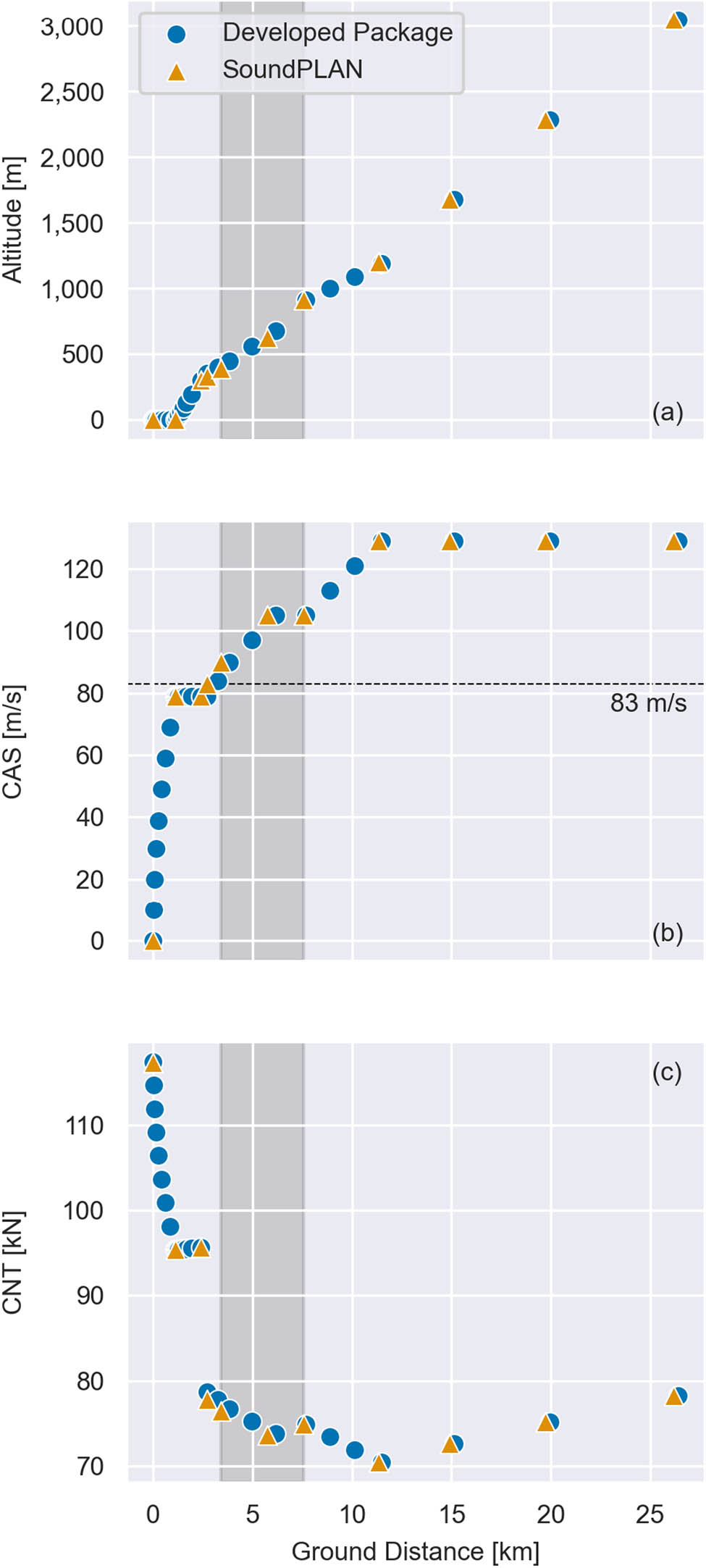
Figures 5 and 6 show the departure and arrival flight profiles, respectively, obtained from our developed package and SoundPLAN. A subplot is dedicated to every parameter (altitude, CAS, and CNT) to illustrate their changes relative to ground distance. In both figures, it can be observed that our developed package could produce results comparable to the benchmark in scenarios involving turboprop aircraft.

Departure flight profiles of the C-130 turboprop aircraft obtained from our developed package and SoundPLAN, showing (a) altitude, (b) CAS, and (c) CNT vs ground distance. Smaller shaded region denotes the takeoff ground roll. Larger shaded region denotes the start of the third step to the end of the fourth step in the flight procedures (Table A2).

Arrival flight profiles of the C-130 turboprop aircraft obtained from our developed package and SoundPLAN, showing (a) altitude, (b) CAS, and (c) CNT vs ground distance. Shaded region denotes the final descent.
Specific to departure, the data points for altitude, ground distance, and CAS deviated from the benchmark over a range of
The data points for CNT deviated from the benchmark over a range of
Specific to arrival, the data points for altitude were in excellent agreement with the benchmark, having no discrepancies (Figure 6a). The data points for ground distance and CAS deviated from the benchmark over a range of
For CNT, the data points deviated from the benchmark over a range of
The data points after the final descent contributed to the positive discrepancies. Small discrepancies (2.6%) were observed for the two data points at the start of the final descent and at the touchdown point. The main contributors to the discrepancies (13.7%) were the data points at the thrust reversal point and the taxiing point. For both data points, our developed package computed the CNT according to the recommendations in the flight procedures (Table A3). As such, the CNT at the thrust reversal point should be 40% (14.3 kN) of the maximum sea-level static thrust (35.7 kN). At the taxiing point, the CNT should be 10% (3.6 kN) of the maximum sea-level static thrust (35.7 kN). Our investigations uncovered that SoundPLAN computed the respective CNT values using 35% (12.5 kN) and 8.8% (3.1 kN) instead of 40% and 10%. As the latter pair is also recommended in ECAC Doc 29 Vol 2 as a generalised approach, our developed package maintained consistency with the recommendations in the flight procedures.
3.2.2 Turbofan aircraft (737-8 MAX)
Presented in the same manner, Figures 7 and 8 show the departure and arrival flight profiles, respectively, obtained from our developed package and SoundPLAN. In both figures, it can be observed that our developed package could produce highly reliable results in scenarios involving turbofan aircraft.
Departure flight profiles of the 737-8 MAX turbofan aircraft obtained from our developed package and SoundPLAN, showing (a) altitude, (b) CAS, and (c) CNT vs ground distance. Shaded region denotes the start of the third step to the end of the fourth step in the flight procedures (Table A4).

Arrival flight profiles of the 737-8 MAX turbofan aircraft obtained from our developed package and SoundPLAN, showing (a) altitude, (b) CAS, and (c) CNT vs ground distance. Shaded region denotes the start of the second step to the end of the fourth step in the flight procedures (Table A5).
Specific to departure, the data points for CNT agreed very well with the benchmark, deviating over a range of
The data points for ground distance deviated from the benchmark over a range of 0–7.3%. Large discrepancies were observed between the third and fourth steps in the flight procedures (Table A4). As discussed in Section 3.2.1, the observation might be caused by the differences in how the iterative loops were coded compared to SoundPLAN. Similarly, large discrepancies were observed at the same data points for altitude. Overall, the data points deviated from the benchmark over a range of
Specific to arrival, the data points for ground distance, altitude, and CAS agreed very well with the benchmark, deviating over a range of
The upper limit (9.6%) was contributed by the overestimation at the start of the final descent. In our developed package, the CNT (24.8 kN) was computed from equation (9) by having
3.3 Benchmarking the overall noise maps
Having established the reliability of the output produced by Module 1, the output of Module 2 was next benchmarked against SoundPLAN. Module 3 was used to generate the overall noise maps. Positional noise maps are not presented in this section because there were more than 20 frames involved in generating them (GIF files). Here, we present the noise maps in two sections to differentiate between turboprop (Section 3.3.1) and turbofan (Section 3.3.2) aircraft. For ease of interpretation, the noise maps (
3.3.1 Turboprop aircraft (C-130)
Figures 9 and 10 show the departure and arrival noise maps, respectively, obtained from our developed package and SoundPLAN. Both figures demonstrate the capability of our developed package to generate noise maps with accuracy comparable to the benchmark in scenarios involving turboprop aircraft. Given the strong agreement between the arrival noise maps, the following discussions will focus on departure.
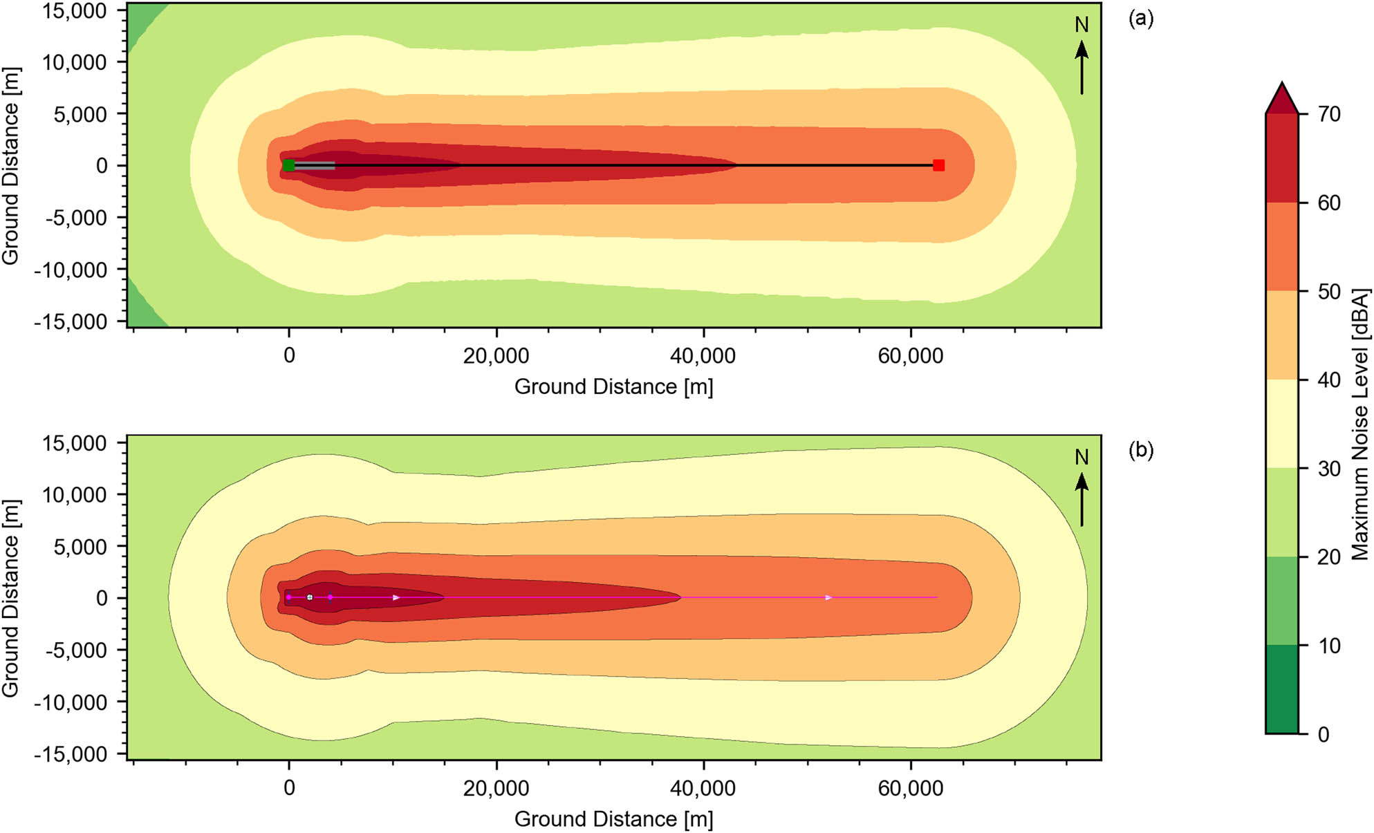
Departure noise maps of the C-130 turboprop aircraft: (a) our developed package and (b) SoundPLAN. In (a), green and red squares denote the start and end of the flight path (black solid line), respectively. The grey solid line denotes the runway.

Arrival noise maps of the C-130 turboprop aircraft: (a) our developed package and (b) SoundPLAN. In (a), green and red squares denote the start and end of the flight path (black solid line), respectively. The grey solid line denotes the runway.
Let us first direct our focus on the region of the noise map that is in front of the runway (
Next, let us direct our focus on the region of the noise map that is behind the runway (
3.3.2 Turbofan aircraft (737-8 MAX)
Figures 11 and 12 show the departure and arrival noise maps, respectively, obtained from our developed package and SoundPLAN. Again, both figures demonstrate the capability of our developed package to generate noise maps with accuracy comparable to the benchmark in scenarios involving turbofan aircraft. Given the strong agreement between the departure noise maps, the following discussions will focus on arrival.

Departure noise maps of the 737-8 MAX turbofan aircraft: (a) our developed package and (b) SoundPLAN. In (a), green and red squares denote the start and end of the flight path (black solid line), respectively. The grey solid line denotes the runway.

Arrival noise maps of the 737-8 MAX turbofan aircraft: (a) our developed package and (b) SoundPLAN. In (a), green and red squares denote the start and end of the flight path (black solid line), respectively. The grey solid line denotes the runway.
Between
Selected noise–power–distance (NPD) values (converted to metric units) of the 737-8 MAX turbofan aircraft [53]
| Direct distance (m) | |||
|---|---|---|---|
| CNT (kN) | 610 (dBA) | 1,219 (dBA) | 1,920 (dBA) |
| 13,345 | 65.9 | 57.1 | 50.7 |
| 17,793 | 65.9 | 57.1 | 50.6 |
| 22,241 | 66.1 | 57.2 | 50.7 |
| 26,689 | 66.5 | 57.6 | 51.0 |
Direct distance is measured from the aircraft to the receiver. Noise levels are expressed in
4 Discussion of the main limitations
In software development, limitations are necessary to shape the latest version so that design objectives can be achieved. These limitations can be associated with technical constraints, budgetary constraints, time constraints, and scope constraints. On the flip side, limitations can help prioritise enhancements for future work. As the software receives new updates through successive development cycles, it will gradually improve. In this section, the main limitations of our developed package are discussed, providing potential enhancements to consider for future work.
4.1 Supporting other noise metrics
For non-specialists, the
4.2 Supporting multiple-event scenarios
At times, our target users may wish to conduct noise impact assessments for a multiple-event scenario, which involves more than one departure or arrival. In contrast, a single-event scenario allows only one departure or arrival to be considered. For example, a multiple-event scenario can provide a more comprehensive description of the flight operations at an international airport. This enhancement will mainly impact Module 1. In practice, each aircraft may deviate from the intended flight path to some extent, especially during the initial climb. Collectively, the deviations contribute to the lateral spreading of ground tracks perpendicular to the intended ground track. ECAC Doc 29 Vol 2 specifies that the deviations were found to follow a Gaussian distribution with the main flight at the centre. Hence, Module 1 will need a new set of algorithms to account for ground track spreading, apart from extracting more aircraft data from the embedded database.
4.3 Combining departure and arrival scenarios
If multiple-event scenarios can eventually be supported, our target users may be interested in studying the combined effects of multiple departing and arriving flights within the same scenario. Currently, our developed package can only consider departing and arriving flights as independent scenarios. Again, Module 1 will be largely impacted by this enhancement. In addition to what was discussed in Section 4.2, Module 1 will need another set of algorithms to correctly merge both departure and arrival flight profiles (spatial information and values of the performance parameters).
4.4 Displaying safety noise limits
When noise maps are generated, our target users may not always be certain of the safety noise limits, which determine whether the neighbourhood may be facing potential noise issues. These noise limits can vary depending on the regulations that local authorities take reference from. Therefore, displaying the noise limits with respect to the local regulations in the GUI is believed to benefit our target users. However, it is also important to note that this enhancement will only be possible if the corresponding noise metrics are supported in the first place. This enhancement will particularly impact Module 3, which is responsible for handling the visual aspects of the noise maps.
4.5 Calculating facade noise level
If our target users aim to evaluate the noise impact within an existing neighbourhood, our developed package currently lacks the ability to account for the physical existence of buildings. In densely populated urban areas, having existing buildings in the study area is nearly unavoidable. Thus, incorporating the representation of buildings into our developed package is a crucial priority. Furthermore, the capability to calculate noise levels specifically on building facades becomes essential for subsequent studies pertaining to noise mitigation within residential spaces. This enhancement will impact Modules 2 and 3. In particular, Module 2 will need a new set of algorithms responsible for importing three-dimensional building models, generating facade nodes, and calculating nodal noise levels while accounting for the relevant sound propagation physics.
5 Conclusion
In conclusion, this article has presented the development and benchmarking of a package designed to easily generate aircraft noise maps via simplified procedures and a reduced amount of input data, with acceptable accuracy in the results. These benefits distinguish our developed package from commercial software. However, we must stress that the results produced by our developed package are intended primarily for quick evaluation and should be regarded as approximate. Ultimately, it is advisable to validate the results through field measurement data and benchmarking with commercial software tailored for comprehensive noise calculations. Our developed package was eventually integrated into an in-house-developed unified urban environmental modelling tool that aims to help urban planners design more liveable and sustainable residential towns in an intuitive and quick manner. By regularly seeking feedback from our target users through trial runs, future work will help address the current limitations and improve the GUI and functionality of our developed package. When ready, we can consider the unified urban environmental modelling tool for external use.
Acknowledgements
We would like to thank Mr. Senthil Kumar Selvara and Ms. Fiona Liausvia from the Institute of High Performance Computing, A*STAR, for working closely with us to design and develop the GUI specific to the aircraft noise mapping feature.
-
Funding information: This research is supported by the National Research Foundation, Singapore.
-
Author contributions: L.Y.L.A.: conceptualisation, methodology, software, benchmarking, formal analysis, data curation, writing – original draft, visualisation. F.C.: conceptualisation, methodology, resources, writing – review & editing, supervision, project administration, funding acquisition. H.J.P.: resources, writing – review & editing, supervision, project administration, funding acquisition.
-
Conflict of interest: We declare no known competing financial interests or personal relationships that could have appeared to influence the research reported in this article.
-
Data availability statement: The data generated in this research are not made available publicly.
Appendix A Default values of the essential parameters
This section provides supplementary information on the default values of the essential parameters given to the user in the GUI (Table A1). Unlike commercial software, our developed package can easily generate reliable noise maps as long as the user selects the aircraft model and the flight type. Although imperial units are preferred in the aviation sector, the GUI was designed with ease of use in mind, using metric units for all inputs. Units are converted in the back-end.
Default values of the essential parameters given to the user in the GUI
| Module | Parameter | Value | Unit |
|---|---|---|---|
| 1 | Ambient air pressure | 101.325 | kPa |
| Ambient air temperature | 15 |
|
|
| Headwind | 4.12 | m/s | |
| Runway elevation | 0 | m | |
| Runway gradient | 0 | — | |
| Runway length | 4,000 | m | |
| Runway heading | 90 |
|
|
| 2 | Plane type | Automatic | — |
| Plane altitude | 0 | m | |
| Grid size | 304.8 | m | |
| Lateral coverage factor | 0.25 | — | |
| 3 | Contour range | 0–70 | dBA |
| Contour interval | 5 | dBA | |
| Aspect ratio | Equal axes | — | |
| Display runway | Yes | — | |
| Display ground track | Yes | — |
B Default flight procedures
For every aircraft, the manufacturer publishes the default flight procedures that can be used as a reference to how the aircraft is being operated during departure or arrival. This section provides the supplementary information on the default flight procedures (departure and arrival) [53] for the C-130 aircraft (Tables A2 and A3) and 737-8 MAX aircraft (Tables A4 and A5).
Default flight procedures for the C-130 aircraft during departure
| No. | Step type | Thrust rating | Final altitude (ft) | ROC (ft/min) | Final CAS (kt) |
|---|---|---|---|---|---|
| 1 | Ground roll | Max takeoff | |||
| 2 | Initial climb | Max takeoff | 1,000 | ||
| 3 | Acceleration | Max takeoff | 1,423 | 142 | |
| Transition step for thrust cutback | |||||
| 4 | Acceleration | Max climb | 1,068 | 162 | |
| 5 | Constant speed | Max climb | 3,000 | ||
| 6 | Acceleration | Max climb | 1,000 | 200 | |
| 7 | Constant speed | Max climb | 5,500 | ||
| 8 | Constant speed | Max climb | 7,500 | ||
| 9 | Constant speed | Max climb | 10,000 | ||
ROC and CAS denote the rate of climb and the calibrated airspeed, respectively.
Default flight procedures for the C-130 aircraft during arrival
| No. | Step type | Initial altitude (ft) | Initial CAS (kt) | Descent angle (deg) | Distance (ft) | Initial thrust (%) |
|---|---|---|---|---|---|---|
| 1 | Descent | 6,000 | 200 | 3 | ||
| 2 | Descent | 3,000 | 166 | 3 | ||
| 3 | Descent | 1,500 | 146 | 3 | ||
| 4 | Final descent | 1,000 | 136 | 3 | ||
| 5 | Touchdown | 341 | ||||
| 6 | Ground roll | 129 | 3,070 | 40 | ||
| 7 | Taxiing | 30 | 10 |
CAS denotes the calibrated airspeed.
Default flight procedures for the 737-8 MAX aircraft during departure
| No. | Step type | Thrust rating | Final altitude (ft) | ROC (ft/min) | Final CAS (kt) |
|---|---|---|---|---|---|
| 1 | Ground roll | Max takeoff | |||
| 2 | Initial climb | Max takeoff | 1,000 | ||
| Transition step for thrust cutback | |||||
| 3 | Acceleration | Max climb | 1,336 | 174 | |
| 4 | Acceleration | Max climb | 1,799 | 205 | |
| 5 | Constant speed | Max climb | 3,000 | ||
| 6 | Acceleration | Max climb | 1,681 | 250 | |
| 7 | Constant speed | Max climb | 5,500 | ||
| 8 | Constant speed | Max climb | 7,500 | ||
| 9 | Constant speed | Max climb | 10,000 | ||
ROC and CAS denote the rate of climb and the calibrated airspeed, respectively.
Default flight procedures for the 737-8 MAX aircraft during arrival
| No. | Step type | Initial altitude (ft) | Initial CAS (kt) | Descent angle (deg) | Distance (ft) | Initial thrust (%) |
|---|---|---|---|---|---|---|
| 1 | Descent | 6,000 | 250 | 3 | ||
| 2 | Level | 3,000 | 250 | 24,557 | ||
| 3 | Level | 3,000 | 189 | 4,678 | ||
| 4 | Level | 3,000 | 174 | 4,907 | ||
| 5 | Descent | 3,000 | 152 | 3 | ||
| 6 | Final descent | 2,817 | 139 | 3 | ||
| 7 | Touchdown | 394 | ||||
| 8 | Ground roll | 139 | 3,838 | 40 | ||
| 9 | Taxiing | 30 | 10 |
CAS denotes the calibrated airspeed.
References
[1] Asdrubali F, D’Alessandro F. Innovative approaches for noise management in smart cities: A review. Current Pollution Reports. 2018;4(2):143–53. 10.1007/s40726-018-0090-zSearch in Google Scholar
[2] Liu Y, Ma X, Shu L, Yang Q, Zhang Y, Huo Z, et al. Internet of Things for noise mapping in smart cities: State of the art and future directions. IEEE Network. 2020;34(4):112–8. 10.1109/MNET.011.1900634Search in Google Scholar
[3] Alias F, Alsina-Pagés RM. Review of wireless acoustic sensor networks for environmental noise monitoring in smart cities. J Sensors. 2019;2019:1–13. 10.1155/2019/7634860Search in Google Scholar
[4] Licitra G, Artuso F, Bernardini M, Moro A, Fidecaro F, Fredianelli L. Acoustic beamforming algorithms and their applications in environmental noise. Current Pollution Reports. 2023;9(3):486–509. 10.1007/s40726-023-00264-9Search in Google Scholar
[5] Shah SK, Tariq Z, Lee J, Lee Y. Real-time machine learning for air quality and environmental noise detection. In: Proceedings of the 2020 IEEE International Conference on Big Data (Big Data). Atlanta, GA, USA: IEEE; 2020. p. 3506–15. 10.1109/BigData50022.2020.9377939Search in Google Scholar
[6] Renaud J, Karam R, Salomon M, Couturier R. Deep learning and gradient boosting for urban environmental noise monitoring in smart cities. Expert Syst Appl. 2023;218:119568. 10.1016/j.eswa.2023.119568Search in Google Scholar
[7] Nourani V, Gökçekuş H, Umar IK. Artificial intelligence based ensemble model for prediction of vehicular traffic noise. Environ Res. 2020;180:108852. 10.1016/j.envres.2019.108852Search in Google Scholar PubMed
[8] Fredianelli L, Carpita S, Bernardini M, Del Pizzo LG, Brocchi F, Bianco F, et al. Traffic flow detection using camera images and machine learning methods in its for noise map and action plan optimisation. Sensors. 2022;22(5):1929. 10.3390/s22051929Search in Google Scholar PubMed PubMed Central
[9] López JM, Alonso J, Asensio C, Pavón I, Gascó L, De Arcas G. A digital signal processor based acoustic sensor for outdoor noise monitoring in smart cities. Sensors. 2020;20(3):605. 10.3390/s20030605Search in Google Scholar PubMed PubMed Central
[10] Ballesteros JA, Sarradj E, Fernández MD, Geyer T, Ballesteros MJ. Noise source identification with beamforming in the pass-by of a car. Appl Acoustics. 2015;93:106–19. 10.1016/j.apacoust.2015.01.019Search in Google Scholar
[11] Pallas MA, Bérengier M, Chatagnon R, Czuka M, Conter M, Muirhead M. Towards a model for electric vehicle noise emission in the European prediction method CNOSSOS-EU. Appl Acoustics. 2016;113:89–101. 10.1016/j.apacoust.2016.06.012Search in Google Scholar
[12] Licitra G, Bernardini M, Moreno R, Bianco F, Fredianelli L. CNOSSOS-EU coefficients for electric vehicle noise emission. Appl Acoustics. 2023;211:109511. 10.1016/j.apacoust.2023.109511Search in Google Scholar
[13] Steinbach L, Altinsoy ME. Prediction of annoyance evaluations of electric vehicle noise by using artificial neural networks. Appl Acoustics. 2019;145:149–58. 10.1016/j.apacoust.2018.09.024Search in Google Scholar
[14] Ascari E, Cerchiai M, Fredianelli L, Melluso D, Rampino F, Licitra G. Decision trees and labeling of low noise pavements as support for noise action plans. Environ Pollution. 2023;337:122487. 10.1016/j.envpol.2023.122487Search in Google Scholar PubMed
[15] Ascari E, Cerchiai M, Fredianelli L, Licitra G. Statistical pass-by for unattended road traffic noise measurement in an urban environment. Sensors. 2022;22(22):8767. 10.3390/s22228767Search in Google Scholar PubMed PubMed Central
[16] Smite D, Moe NB, Hildrum J, Gonzalez-Huerta J, Mendez D. Work-from-home is here to stay: Call for flexibility in post-pandemic work policies. J Syst Softw. 2023;195:111552. 10.1016/j.jss.2022.111552Search in Google Scholar PubMed PubMed Central
[17] George TJ, Atwater LE, Maneethai D, Madera JM. Supporting the productivity and wellbeing of remote workers: Lessons from COVID-19. Organisational Dynam. 2022;51(2):100869. 10.1016/j.orgdyn.2021.100869Search in Google Scholar PubMed PubMed Central
[18] Wothge J, Belke C, Möhler U, Guski R, Schreckenberg D. The combined effects of aircraft and road traffic noise and aircraft and railway noise on noise annoyance–An analysis in the context of the joint research initiative NORAH. Int J Environ Res Public Health. 2017;14(8):871. 10.3390/ijerph14080871Search in Google Scholar PubMed PubMed Central
[19] Schäffer B, Brink M, Schlatter F, Vienneau D, Wunderli JM. Residential green is associated with reduced annoyance to road traffic and railway noise but increased annoyance to aircraft noise exposure. Environ Int. 2020;143:105885. 10.1016/j.envint.2020.105885Search in Google Scholar PubMed
[20] WHO. Environmental Noise Guidelines for the European Region. Copenhagen, Denmark: World Health Organisation; 2019. Search in Google Scholar
[21] Beutel ME, Jünger C, Klein EM, Wild P, Lackner K, Blettner M, et al. Noise annoyance is associated with depression and anxiety in the general population–The contribution of aircraft noise. PLoS One. 2016;11(5):e0155357. 10.1371/journal.pone.0155357Search in Google Scholar PubMed PubMed Central
[22] Ang LYL, Cui F. Remote work: Aircraft noise implications, prediction, and management in the built environment. Appl Acoustics. 2022;198:108978. 10.1016/j.apacoust.2022.108978Search in Google Scholar PubMed PubMed Central
[23] Sparrow V, Gjestland T, Guski R, Richard, Basner M, Hansell A, et al. State of the science 2019: Aviation noise impacts. In: ICAO Environmental Report 2019. Montreal, Canada: International Civil Aviation Organisation; 2019. p. 44–61. Search in Google Scholar
[24] Babisch W. Updated exposure-response relationship between road traffic noise and coronary heart diseases: A meta-analysis. Noise Health. 2014;16(68):1–9. 10.4103/1463-1741.127847Search in Google Scholar PubMed
[25] Cohen JP, Coughlin CC. Spatial hedonic models of airport noise, proximity, and housing prices. J Regional Sci. 2008;48(5):859–78. 10.1111/j.1467-9787.2008.00569.xSearch in Google Scholar
[26] O’Byrne PH, Nelson JP, Seneca JJ. Housing values, census estimates, disequilibrium, and the environmental cost of airport noise: A case study of Atlanta. J Environ Econ Manag. 1985;12(2):169–78. 10.1016/0095-0696(85)90026-9Search in Google Scholar
[27] Mahmoud NSA, Jung C, Al Qassimi N. Evaluating the aircraft noise level and acoustic performance of the buildings in the vicinity of Dubai International Airport. Ain Shams Eng J. 2023;14(8):102032. 10.1016/j.asej.2022.102032Search in Google Scholar
[28] Bueno AM, de Paula Xavier AA, Broday EE. Evaluating the connection between thermal comfort and productivity in buildings: A systematic literature review. Buildings. 2021;11(6):244. 10.3390/buildings11060244Search in Google Scholar
[29] Postorino MN, Mantecchini L. A systematic approach to assess the effectiveness of airport noise mitigation strategies. J Air Transport Manag. 2016;50:71–82. 10.1016/j.jairtraman.2015.10.004Search in Google Scholar
[30] Licitra G, Gagliardi P, Fredianelli L, Simonetti D. Noise mitigation action plan of Pisa civil and military airport and its effects on people exposure. Appl Acoustics. 2014;84:25–36. 10.1016/j.apacoust.2014.02.020Search in Google Scholar
[31] Behere A, Mavris DN. Optimisation of takeoff departure procedures for airport noise mitigation. Trans Res Record J Transport Res Board. 2021;2675(9):81–92. 10.1177/03611981211004967Search in Google Scholar
[32] Gagliardi P, Fredianelli L, Simonetti D, Licitra G. ADS-B system as a useful tool for testing and redrawing noise management strategies at Pisa Airport. Acta Acustica united with Acustica. 2017;103(4):543–51. 10.3813/AAA.919083Search in Google Scholar
[33] Arafa MH, Osman TA, Abdel-Latif IA. Noise assessment and mitigation schemes for Hurghada Airport. Appl Acoustics. 2007;68(11–12):1373–85. 10.1016/j.apacoust.2006.08.004Search in Google Scholar
[34] Yang YL. Comparison of public perception and risk management decisions of aircraft noise near Taoyuan and Kaohsiung International Airports. J Air Transport Manag. 2020;85:101797. 10.1016/j.jairtraman.2020.101797Search in Google Scholar
[35] Kwak KM, Ju YS, Kwon YJ, Chung YK, Kim BK, Kim H, et al. The effect of aircraft noise on sleep disturbance among the residents near a civilian airport: A cross-sectional study. Annal Occupat Environ Med. 2016;28(1):38. 10.1186/s40557-016-0123-2Search in Google Scholar PubMed PubMed Central
[36] Choy J. Mitigating the impact of Tengah Airbase on residences [Bachelor’s Thesis]. Republic of Singapore: National University of Singapore; 2020. https://scholarbank.nus.edu.sg/handle/10635/220285. Search in Google Scholar
[37] Lee HP, Kumar S, Garg S, Lim KM. Characteristics of aircraft flypast noise around Singapore Changi International Airport. Appl Acoustics. 2022;185:108418. 10.1016/j.apacoust.2021.108418Search in Google Scholar
[38] Di G, Liu X, Shi X, Li Z, Lin Q. Investigation of the relationship between aircraft noise and community annoyance in China. Noise Health. 2012;14(57):52. 10.4103/1463-1741.95132Search in Google Scholar PubMed
[39] Basner M, Barnett I, Carlin M, Choi GH, Czech JJ, Ecker AJ, et al. Effects of aircraft noise on sleep: Federal Aviation Administration National Sleep Study protocol. Int J Environ Res Public Health. 2023;20(21):7024. 10.3390/ijerph20217024Search in Google Scholar PubMed PubMed Central
[40] Heinonen-Guzejev M, Vuorinen HS, Kaprio J, Heikkilä K, Mussalo-Rauhamaa H, Koskenvuo M. Self-report of transportation noise exposure, annoyance and noise sensitivity in relation to noise map information. J Sound Vibration. 2000;234(2):191–206. 10.1006/jsvi.1999.2885Search in Google Scholar
[41] King EA, Rice HJ. The development of a practical framework for strategic noise mapping. Appl Acoustics. 2009;70(8):1116–27. 10.1016/j.apacoust.2009.01.005Search in Google Scholar
[42] Wunderli JM, Zellmann C, Köpfli M, Habermacher M. sonAIR-A GIS-integrated spectral aircraft noise simulation tool for single flight prediction and noise mapping. Acta Acustica united with Acustica. 2018;104(3):440–51. 10.3813/AAA.919180Search in Google Scholar
[43] Jäger D, Zellmann C, Schlatter F, Wunderli JM. Validation of the sonAIR aircraft noise simulation model. Noise Mapping. 2021;8(1):95–107. 10.1515/noise-2021-0007Search in Google Scholar
[44] Meister J, Schalcher S, Wunderli JM, Jäger D, Zellmann C, Schäffer B. Comparison of the aircraft noise calculation programs sonAIR, FLULA2, and AEDT with noise measurements of single flights. Aerospace. 2021;8(12):388. 10.3390/aerospace8120388Search in Google Scholar
[45] Riboldi CED, Trainelli L, Mariani L, Rolando A, Salucci F. Predicting the effect of electric and hybrid-electric aviation on acoustic pollution. Noise Mapping. 2020;7(1):35–56. 10.1515/noise-2020-0004Search in Google Scholar
[46] ECAC. ECAC Doc 29 Vol 1: Report on Standard Method of Computing Noise Contours Around Civil Airports–Applications Guide. 4th ed. Neuilly-sur-Seine, France: European Civil Aviation Conference; 2016. Search in Google Scholar
[47] ECAC. ECAC Doc 29 Vol 2: Report on Standard Method of Computing Noise Contours Around Civil Airports–Technical Guide. 4th ed. Neuilly-sur-Seine, France: European Civil Aviation Conference; 2016. Search in Google Scholar
[48] ECAC. ECAC Doc 29 Vol 3 Part 1: Report on Standard Method of Computing Noise Contours Around Civil Airports–Reference Cases and Verification Framework. 4th ed. Neuilly-sur-Seine. 4th ed. Neuilly-sur-Seine, France: European Civil Aviation Conference; 2016. Search in Google Scholar
[49] EU. Directive 2002/49/EC: Assessment and Management of Environmental Noise. Brussels, Belgium: European Union; 2002. Search in Google Scholar
[50] Yang C, Mott JH. Developing a cost-effective assessment method for noise impacts at non-towered airports: A case study at Purdue University. Transport Res Record J Transport Res Board. 2022;2676(12):786–97. 10.1177/03611981221097705Search in Google Scholar
[51] Nakazawa T, Sugawara M, Shinohara N, Yamada I. Difference in airport noise calculation procedures between AERC model and ECAC Doc 29. In: Proceedings of the 46th International Congress and Exposition on Noise (INTER-NOISE 2017). Hong Kong, China: Institute of Noise; 2017. p. 2640. Search in Google Scholar
[52] Liu V. Researchers who created urban planning simulation model for Tengah wins President’s Technology Award. The Straits Times. 2019. Accessed Jul 1, 2023. https://www.straitstimes.com/singapore/researchers-who-created-urban-planning-simulation-model-for-tengah-wins-presidents. Search in Google Scholar
[53] EUROCONTROL. The Aircraft Noise and Performance (ANP) Database: An international data resource for aircraft noise modellers. EUROCONTROL. 2020. Accessed Jul 1, 2023. https://www.aircraftnoisemodel.org/. Search in Google Scholar
[54] ISO. ISO 2533: Standard Atmosphere. Geneva, Switzerland: International Organisation for Standardisation; 1975. Search in Google Scholar
© 2024 the author(s), published by De Gruyter
This work is licensed under the Creative Commons Attribution 4.0 International License.
Articles in the same Issue
- Regular Articles
- Low-frequency cabin noise of rapid transit trains
- Utilizing the phenomenon of diffraction for noise protection of roadside objects
- Benchmarking the aircraft noise mapping package developed for a unified urban environmental modelling tool
- Acoustical analysis and optimization design of the hair dryers
- Methodologies for the prediction of future aircraft noise level
- Basics of meteorology for outdoor sound propagation and related modelling issues
- Predictive noise annoyance and noise-induced health effects models for road traffic noise in NCT of Delhi, India
- Modeling and mapping of traffic noise pollution by ArcGIS and TNM2.5 techniques
- A novel method for constructing large-scale industrial noise maps based on open source data
- Understanding perceived tranquillity in urban Woonerf streets: case studies in two Dutch cities
- Review Article
- A comprehensive review of noise pollution monitoring studies at bus transit terminals
- Rapid Communication
- The Environment (Air Quality and Soundscapes) (Wales) Act 2024
- Erratum
- Erratum to “Comparing pre- and post-pandemic greenhouse gas and noise emissions from road traffic in Rome (Italy): a multi-step approach”
- Special Issue: Latest Advances in Soundscape - Part II
- Soundscape maps of pleasantness in a university campus by crowd-sourced measurements interpolation
- Conscious walk assessment for the joint evaluation of the soundscape, air quality, biodiversity, and comfort in Barcelona
- A framework to characterize and classify soundscape design practices based on grounded theory
- Perceived quality of a nighttime hospital soundscape
- Relating 2D isovists to audiovisual assessments of two urban spaces in a neighbourhood
- Special Issue: Strategic noise mapping in the CNOSSOS-EU era - Part I
- Analysis of road traffic noise in an urban area in Croatia using different noise prediction models
- Citizens’ exposure to predominant noise sources in agglomerations