
NKG2020 transformation: An updated transformation between dynamic and static reference frames in the Nordic and Baltic countries
-
Pasi Häkli
 ,
Kristian Evers
,
Kristian Evers

Abstract
Coordinates in global reference frames are becoming more and more common in positioning whereas most of the geospatial data are stored in registries in national reference frames. It is therefore essential to know the relation between global and national coordinates, i.e., the transformation, as accurately as possible. Officially provided pan-European transformations do not account for the special conditions in the Nordic and Baltic countries, namely crustal deformations caused by Glacial Isostatic Adjustment. Therefore, they do not fulfill the demands for the most accurate applications like long-term reference frame maintenance. Consequently, the Nordic Geodetic Commission (NKG) has developed customized and accurate transformations from the global ITRF to the national ETRS89 realizations for the Nordic and Baltic countries. We present the latest update, called the NKG2020 transformation, with several improvements and uncertainty estimates. We also discuss its significance and practical implementation for geodetic and geospatial communities.
1 Introduction
Globalization and technological development have their effects also on geospatial data. International data sets and positioning services bring global reference frames more and more often to everyday data analysis. At the same time, demands for positioning accuracy have grown but the geospatial data should be stored in registries in national reference frames. It is therefore essential to know the relation between global and national coordinates, i.e., the transformation, as accurately as possible.
The NKG (Nordic Geodetic Commission) transformation methodology with associated parameters was released in 2016 (Häkli et al. 2016). Its main purpose is to harmonize transformations in the Nordic and Baltic countries and to provide accurate links between global dynamic and national static reference frames. This is particularly important for maintaining static reference frames in the Nordic and Baltic countries. The NKG transformation is time-dependent to account for the time-variable crustal motions. The foundation of the method is the standardized pan-European transformation provided by EUREF (IAG Reference Frame Sub-Commission for Europe) (Altamimi 2018). It includes two steps: global transformations between different ITRS (International Terrestrial Reference System) realizations defined by International Earth Rotation and Reference Systems Service (IERS) and pan-European transformation parameters to comply with the ETRS89 (European Terrestrial Reference System 1989) definitions. The main goal of the EUREF approach is to minimize coordinate changes due to tectonic plate motions using a plate-fixed terrestrial reference frame (TRF). However, the transformation only accounts for the rigid plate motion of the Eurasian plate, and any intra- or inter-plate deformations are not considered. In the Nordic and Baltic countries, Glacial Isostatic Adjustment (GIA), or more generally land uplift, causes crustal deformations that cannot be omitted in the most accurate applications like long-term reference frame maintenance in the region. GIA causes internal deformations to the Eurasian plate that reach up to about 1 cm/year in the vertical, and some mm/year in the horizontal direction (Häkli et al. 2019; Lahtinen et al. 2019; Vestøl et al. 2019; Kierulf et al. 2021). The Nordic and Baltic ETRS89 realizations were established mostly in the 1990s meaning already more than 20 years of deformations compared to present-day coordinates. The magnitude of the GIA effect and the time span mean that these deformations need to be considered in high-accuracy georeferencing applications and maintenance of national reference frames.
Consequently, the Nordic and Baltic countries, in collaboration under the umbrella of the Nordic Geodetic Commission (NKG), have developed land uplift models and transformation procedures to account for the deformations under these special conditions (NKG 2023). The NKG transformation method adds intraplate corrections as well as national transformation parameters to the EUREF transformation to improve the transformation accuracy. One important addition is a common NKG reference frame that is used as a transformation hub for the national ETRS89 realizations. Reasoning and conventions are given by Häkli et al. (2016). This approach was labeled as the NKG2008 transformation, and with it, the transformation accuracy improved from the level of a couple of decimeters (extreme values close to the land uplift maximum region) to (sub-)centimeter level.
Similar approaches have been developed for example in Iceland, New Zealand, and the United States, however with more complex tectonic settings. Icelandic ISN2016 is a semi-dynamic reference frame with the reference epoch 2016.5 and including a deformation model to switch from one epoch to another (Kierulf et al. 2019; Valsson 2021). New Zealand Geodetic Datum 2000 (NZGD2000) is defined through its relationship to ITRF (International Terrestrial Reference Frame) via the deformation model (Crook et al. 2016). Both Iceland and New Zealand are located at the boundary of two major tectonic plates and consequently associated deformation models, and thus, velocities are aligned to ITRF. The United States has chosen an equivalent solution as NKG for their modernized National Spatial Reference System (NSRS). The US territories are spread over several tectonic plates leading to four new plate-fixed reference frames. The basic principle for each frame follows that of the NKG: global ITRF coordinates are reduced to plate-fixed coordinates at the reference epoch. This includes rigid plate motions with the Euler pole parameters (EPP) and intra-plate deformations will be captured by a model called an Intra-Frame Velocity Model (IFVM) (NGS 2021). These examples show that the concept of two-frame approach (also called a semi-dynamic reference frame) (Donnelly et al. 2015) is becoming more common for future modernized national reference frames and their maintenance.
Here, we present the latest update of the NKG transformation, called the NKG2020 transformation. The main motivation to update the NKG transformation is the availability of new fundamental data sets that enable improved accuracy. Since the NKG2008 transformation, NKG has released new GIA models and multiyear GNSS solutions (Lahtinen et al. 2019, 2022; Kierulf et al. 2021), based on such data sets new land uplift models NKG2016LU (Vestøl et al. 2019) and NKG_RF17vel (Häkli et al. 2019). NKG2016LU and NKG_RF17vel land uplift models provide fundamental improvements over the previously used models NKG2005LU (Vestøl 2006) and NKG_RF03vel (Nørbech et al. 2006). Additionally, the ITRF coordinates used for determining the previous NKG2008 transformation parameters were based on the coordinates of the NKG2008 GPS campaign (Jivall et al. 2010) whereas now a multiyear ITRF2014 coordinate and velocity solution with much better quality and uncertainty estimates were available (Lahtinen et al. 2019). Moreover, many Nordic and Baltic countries have made updates to their ETRS89 coordinates and even calculated new realizations. Hence, both input coordinate sets have been revised and have improved quality. The NKG2020 methodology follows that of the NKG2008 transformation, but all data needed for determining the transformation, i.e., input coordinates and the land uplift model, were revised and updated resulting in an optimal transformation accuracy.
In Section 2, we briefly describe the improvements in the methodology. The NKG2020 transformation is a major update with all data being revised and updated. In Section 3, we present the used data that the transformation relies upon. In Section 4, we give the results and compare them to the previous version, NKG2008. We improve the estimation of the transformation uncertainty that is thoroughly discussed in Section 5. Conclusions and discussion are given in Section 6.
2 Methodology
In this section, we give an overview of the NKG2020 transformation steps together with the necessary equations for performing the transformation. Additionally, we describe the methods for estimating the transformation parameters and residuals as well as the method for producing the alternative correction grid. Finally, we describe how we estimated the uncertainties for the NKG2020 transformation.
2.1 NKG transformation
The NKG transformation methodology with associated parameters was published and presented by Häkli et al. (2016). Here, we followed the NKG transformation methodology but updated all associated data for determining a new updated transformation. The new version was labeled as the NKG2020 transformation. The main principle of the NKG2020 transformation remains the same as in the NKG2008 transformation, but the new data resulted in some changes. For determining the NKG2020 transformation parameters, we took the input coordinates from a multiyear GNSS (Global Navigation Satellite System) reference frame solution instead of a GPS (Global Positioning System) campaign that was used in the NKG2008 transformation. The multiyear NKG Repro1 solution (Lahtinen et al. 2019) was processed, and the coordinates and velocities were given in ITRF2014 (Altamimi et al. 2016). Associated intraplate velocities were interpolated from the NKG_RF17vel model, which is aligned to ETRF2014 (European Terrestrial Reference Frame 2014) (Altamimi 2018). According to NKG transformation methodology, this yields that also the transformation hub is aligned to ETRF2014. With this choice, we also avoided unnecessary extra transformations and utilized the latest ETRS89 realization. In the NKG2008 transformation, the intraplate velocities and the transformation hub were aligned to ETRF2000. The origin of the ETRF2014 coincides with that of the ITRF2014 and, therefore, the transformation hub suits better, e.g., for scientific applications like fitting gravimetric geoid models. For the same reason, ETRF2014 differs approximately 5–10 cm from the Nordic–Baltic ETRS89 realizations (which are pre-ETRF2014 realizations) but this still fits perfectly for the purpose. Moreover, all national coordinates were revised and, in many countries, also updated to reflect updates in the national reference frames.
All the new data induced updated national transformations as well. Previously, all national transformations were determined with the seven-parameter Helmert transformation, but as a new method in the NKG2020 transformation the Norwegian transformation is based on a correction grid.
The NKG2020 transformation method is summarized in Figure 1. It is important to note that even if the NKG2020 transformation was determined with the ITRF2014 coordinates, the method supports all ITRF realizations. The first step of the transformation equals the IERS transformation parameters between different ITRFyy realizations, and this enables input coordinates in any of the ITRFyy realizations (IERS 2023 [equation (1)]). This step is not needed if the input coordinates are already in ITRF2014. The second step (equation (2)) transforms the ITRF2014 coordinates to ETRF2014 with the formulae and parameters by EUREF (Altamimi 2018). This step transforms ITRF2014 coordinates at any epoch t to ETRF2014. According to the ETRS89 definition, the coordinates are moved back to epoch 1989.0 but the transformation considers only rigid plate motions, and any intra- or inter-plate deformations are not corrected. These two steps correspond to the EUREF recommendation (Altamimi 2018). The notations in equations (1) and (2) follow that of the IERS conventions (Petit and Luzum 2010) and EUREF Technical Note 1 (Altamimi 2018): T
1, T
2 and T
3 correspond to the translation vectors (origin shifts) along the X-, Y- and Z-axes, R
1, R
2 and R
3 rotations, and
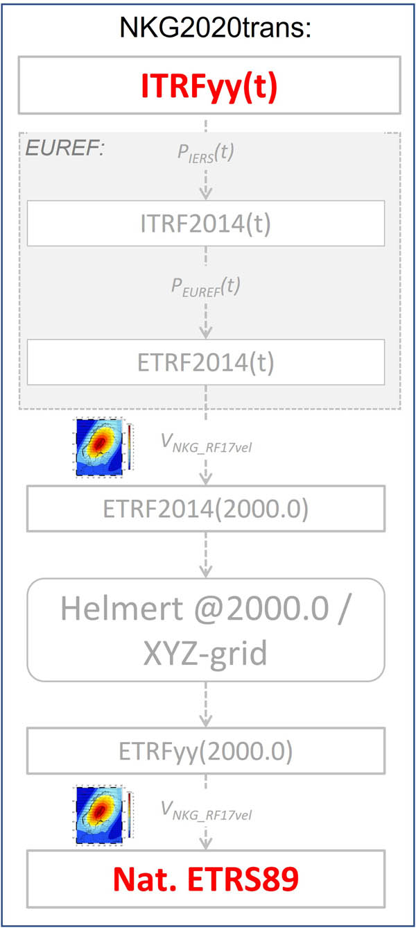
NKG2020 transformation method and the associated steps. The EUREF transformation forms the basis to which additional steps were added to account for the intraplate deformations as well as national reference frames. In the figure, t refers to any coordinate epoch, P IERS refers to the ITRF transformation parameters estimated by IERS, P EUREF to the ETRS89 transformation parameters estimated by EUREF, and V NKG_RF17vel to the intraplate velocities from the NKG_RF17vel model.
The following steps are an add-on to the EUREF recommendation and necessary to account for the intraplate deformations due to the land uplift and possible differences between national and pan-European ETRS89 realizations. The third step accounts for the intraplate deformations with the velocities V from the NKG_RF17vel model and brings ETRF2014 coordinates to the common land uplift epoch 2000.0 (equation (3)). The first three steps are common to all Nordic and Baltic countries, and the resulting ETRF2014 coordinates at epoch 2000.0 constitute a transformation hub that was labeled as NKG_ETRF14. The remaining steps are country specific. The fourth step includes national transformations using either Helmert transformation, equation (4), or interpolation from a correction grid. These transformations correct for the pan-European coordinates to the national reference frames. The final step, equation (5), is yet needed to account for the intraplate deformations between the common epoch 2000.0 and the reference epoch (t r) of the national ETRS89 realizations.
Steps 1–3 constitute the dynamic part of the NKG2020 transformation whereas steps 4–5 remain static (unless possible updates). More details about the background of the transformation steps are discussed by Häkli et al. (2016).
2.2 National transformations: Helmert transformation or least-squares collocation
Typically, three-dimensional transformations have been determined with the seven-parameter (or 14 parameters if rates of parameters are considered) Helmert transformation. The method has also been used for the national transformations in the NKG transformation. The NKG2020 transformation corrects for intraplate deformations with the NKG_RF17vel model but it considers the land uplift (GIA) effects and not deformations or uncertainties in the national reference frames. Subsequent Helmert transformation is a similarity transformation that considers only translation, rotation, and scale of the network. Following the IERS conventions and notations (Petit and Luzum 2010), the three-dimensional similarity transformation can be written with equation (6):
Rewriting equation (6), we get model of observation equations for the Helmert transformation in equation (7):
Observation equation for usual least-squares adjustment by parameters is given with equation (8):
where L is the observation vector, A is the design matrix of observations, x is the unknown Helmert parameters, and ε is the error (residual) of the least-squares adjustment. Omitting the derivation of the equations, we estimated the unknown parameters (or actually their increments) iteratively with equation (9) and finally the transformation errors (residuals) with equation (10) and standard error of unit weight m 0 with equation (11).
In the equations, P is the weight matrix, and n is the number of points. We used equal weights for observations, P = I (identity matrix).
Helmert transformation is a similarity transformation that maintains the shape of the network from the source ITRF2014 solution that is corrected for the GIA effects with the deformation model. As a result, the transformation residuals describe the remaining deformations between the ETRF2014 and national ETRS89 coordinates at the transformation reference epoch 2000.0. Typically, the ITRF coordinates represent the most precise geometry from up-to-date GNSS observations whereas the geometry of national reference frames degrades over time. Consequently, the transformed coordinates inherit the geometry from a GNSS solution, but it may not coincide with the national coordinates good enough. In other words, the transformation does not provide accurate coordinates with respect to the other national geodata infrastructure, which may be a fundamental problem. In such cases, options are to upgrade either the transformation method or the national realization/coordinates. While a national reference frame is a basis for a national geospatial infrastructure, updating a national realization is a huge undertaking with wide consequences and typically not an option.
Determining the NKG2020 transformation for Norway revealed some inhomogeneities in the ETRS89 coordinates of the Norwegian CORS (Continuously Operating Reference Stations) network. The CORS network is the basis for thousands of lower-order passive benchmarks, and altogether, they are the basis for the geospatial data in Norway. Consequently, the residuals of the pure Helmert transformation were considered too large.
To make the residuals smaller, one can add the number of parameters and/or apply more local transformation. Several possible methods exist, for example, TIN (Triangulated Irregular Network)-based transformation used already in Norway and Finland for legacy transformations or transformations based on higher-order polynomials that are used in Denmark. Also, several gridding methods exist like least-squares collocation (LSC) or Kriging. Typically, the legacy methods are complex to implement in practice, but grids are rather easy to use in modern GIS (Geographic Information System) applications. Least-squares collocation is widely used in geodetic applications, and it provides continuous surface over the area of interest. Such a grid corrects for inconsistencies between the input coordinates up to the uncertainty level of the coordinates. Therefore, it can provide more accurate transformed coordinates with respect to the national geospatial infrastructure. Hence, LSC was chosen as the solution in Norway.
Observation equation for the least-squares collocation can be written with equation (12) (Moritz 1980):
The method of the LSC correction grid is a combination of a systematic part Ax, a stochastic part t, and errors n (typically called noise). The systematic part consists of parameters from the seven-parameter Helmert transformation and the stochastic part consists of signals from LSC. The sum of those parts is stored as corrections of a geocentric translation in a final three-dimensional grid. The Helmert parameters are estimated in the same way as in equation (9) but replacing P = C −1 where C is the variance-covariance matrix, leading to equation (13):
Then, the estimated signal at grid points can be estimated with equation (14):
where ŝ is the predicted signal, C st is the covariance matrix between the signals t at observation points and signals s at grid points, and C is the total covariance matrix of the observations L. We estimate C with equation (15):
where C tt is the covariance matrix of the signal t between observation points (here the fiducial points of the transformation) and C nn is the covariance matrix of the noise n (here uncertainties of the fiducial points). Covariance matrices C tt and C st are estimated with a homogeneous and isotropic covariance function assuming that the mean of the random field (of observations) is constant, and the covariances depend only on the (spherical) distance between the points. For this, we used the first-order Gauss–Markov covariance function according to equation (16):
C 0 is the observation variance at d = 0, r is the distance between the points in question, and D is the correlation length. For more details of the least-squares collocation, see e.g. Moritz (1980).
2.3 Uncertainty estimation
In Helmert transformations, residuals describe the consistency between the source and target coordinates and are typically used as an uncertainty estimate for the resulting coordinates and transformation (parameters). In the NKG2020 transformation, both input coordinates are already derived coordinates meaning that they include also uncertainties from the preceding coordinate operations and the original coordinates (Figure 1). For the used data, i.e., the associated coordinate solutions and time intervals, the residuals still describe the total uncertainty. But this is valid only for these specific data, and for other user cases, the data and time intervals are typically different; therefore, the residuals are only a part of the total uncertainty budget. We estimated also other sources of uncertainty to give a more realistic total uncertainty budget for the NKG2020 transformation.
The other uncertainties that should be considered include the source coordinates and the velocity model (for differing correction intervals). The NKG2020 transformation also includes the IERS and the EUREF transformation parameters, but their uncertainties, being a part of the ETRS89 definition, could be considered zero. The total uncertainty can be estimated in many ways, but one exact estimate is difficult to give. One important note is that the NKG2020 transformation is time-dependent and so is its uncertainty. Hence, the uncertainty can be divided into a constant and a time-dependent part. It is also important to remember that the NKG2020 transformation is meant to be an accurate link between the global ITRF and national ETRS89 coordinates for practical applications. Hence, instead of giving a theoretical total uncertainty budget, we decided to estimate the uncertainty empirically.
Our ITRF2014 coordinates for estimating the NKG2020 transformation parameters and the residuals were given at epoch t = 2015.0 (more details in Section 3.2). That can be considered as the epoch for the constant part of the uncertainty (residuals). We assessed the residuals as the uncertainty measure with redundant reference frame (GNSS) solutions and propagated their coordinates to epoch 2015.0. Keeping the epoch t = 2015.0 fixed, the velocity corrections, the national transformation parameters and the national coordinates remain constant, and the additional uncertainties (compared to the residuals) can be attributed to the input ITRF coordinates and, if applicable, to the first transformation step from other ITRF realizations to ITRF2014. Even if the ITRF coordinates typically have variance and covariance information available from GNSS solutions, they are usually quite optimistic, and empirical estimation gives the more realistic picture. We evaluated the constant part with three different reference frame solutions and give an estimate of the uncertainty by analyzing transformation accuracies with respect to the national reference coordinates (Section 5.1).
The time-variable part of the NKG2020 transformation is dominated by the uncertainty of the NKG_RF17vel velocity model. Such models are typically combined from several geodetic data techniques and/or other models, and consequently, also their uncertainty may be difficult to estimate reliably. We provide an estimate for the time-variable part of the uncertainty by transforming coordinates from different epochs to national coordinates. For this, we used ITRF2014 daily coordinate time series that were transformed with the NKG2020 transformation. Then, we analyzed the residual time series in the national ETRS89 realizations (Section 5.2).
We consider that with this methodology we can give more realistic and improved uncertainty estimates for the NKG2020 transformation.
3 Data
The data needed to determine the NKG2020 transformation parameters are input coordinates in ITRF2014 and in national ETRS89 realizations, IERS and EUREF transformation parameters (that are predefined), and corrections from the NKG_RF17vel deformation model.
3.1 National ETRS89 coordinates
Most of the Nordic–Baltic ETRS89 realizations were originally defined in the 1990s. The original realizations were typically defined or at least accessed mostly through passive benchmarks, whereas active CORS (Continuously Operating Reference Stations) networks are dominating today. Due to this and other technological developments, the national ETRS89 realizations have gotten some updates, but normally changes have been small or minimized in the coordinate domain. Some updates have taken place also since the NKG2008 transformation was published in 2016, and this along with some other improvements means that the NKG2020 transformation is a major update and, in most countries, also deprecates the NKG2008 transformation. The national ETRS89 coordinates were evaluated carefully with each Nordic and Baltic country, and they represent the official coordinates of the country for the NKG2020 transformation. Table 1 collects some key details of the Nordic and Baltic ETRS89 realizations as used in the NKG2020 transformation.
National ETRS89 realizations in the Nordic and Baltic countries
| Country | cc | t r | ETRFyy | Name | Reference |
|---|---|---|---|---|---|
| Denmark | DK | 2015.829 | ETRF92 | EUREF-DK94 | (Fankhauser and Gurtner 1995) |
| Estonia | EE | 1997.560 | ETRF96 | EUREF-EST97 | (Rüdja 1999) |
| Finland | FI | 1997.000 | ETRF96 | EUREF-FIN | (Ollikainen et al. 1999, 2000) |
| Latvia | LV | 1992.750 | ETRF89 | LKS-92 | (Madsen and Madsen 1993) |
| Lithuania | LT | 2003.750 | ETRF2000 | LKS 94 (EUREF-NKG-2003) | (Jivall et al. 2007) |
| Norway | NO | 1995.000 | ETRF93 | EUREF89 | (Kristiansen and Harsson 1999) |
| Sweden | SE | 1999.500 | ETRF97 | SWEREF99 | (Jivall and Lidberg 2000) |
3.1.1 Denmark
The Danish ETRS89 realization was originally based on seven passive stations (Fankhauser and Gurtner 1995) which over time have shown some instability. To remedy this, the Danish ETRS89 realization was updated in 2019 to include CORS stations. ETRS89 coordinates for the CORS stations were determined using a Helmert transformation based on the EUREF2015 campaign that included observations of both the original passive stations and the CORS stations. The updated coordinates were determined in 2015, and hence, the intra-plate deformation epoch has changed to 2015.8 from the original epoch of 1992.7. Formally, the realization is unchanged, but in practice, the realization is now carried by the more geodynamically stable CORS stations.
3.1.2 Estonia
The Estonian ETRS89 realization is based on the points of the first-order geodetic network and their coordinates. The coordinates of the ETRS89 implementation are denoted by the abbreviation EUREF-EST97 (Decree of Geodetic system). National CORS network ESTPOS (Metsar et al. 2018) is used to monitor the Estonian geodetic system and its components.
The coordinates of the first-order national geodetic network at epoch 1997.56 are based on IERS 1996 definitions, ITRF96 reference frame, first-order network measurements, and calculation methodology according to the recommendations by EUREF. In order to validate the CORS coordinates, the measurement campaign was held in 2017 (Metsar et al. 2019), which included the first-order national geodetic network points and CORS stations. The campaign resulted in the unified coordinates in the Estonian national geodetic system for the CORS stations. The ESTPOS stations were computed at the epoch 2013.0, and this solution was accepted as EUREF densification for Estonia, corresponding to EUREF Class A accuracy (Kollo et al. 2019). The Estonian geodetic system is defined by the passive geodetic network points (epoch 1997.56) and monitoring is performed by the active geodetic network, i.e., ESTPOS CORS stations (epoch 2013.00).
3.1.3 Finland
The Finnish ETRS89 realization, EUREF-FIN, is based on the GPS campaign measured in 1996–1997. The resulting first-order network covered 12 FinnRef CORS stations and 100 passive ground control points (GCP). The formal accuracy of the EUREF-FIN campaign is at a few millimeter levels (Ollikainen et al. 1999, 2000). This network was later densified with thousands of lower-order GCPs. EUREF-FIN is widely adopted and used as the basis for geospatial data in Finland.
Growing uncertainties in static EUREF-FIN coordinates (e.g., land uplift), technological development (positioning services, connections to international reference frames), and renewal and densification of the active FinnRef CORS network led to a situation where EUREF-FIN (by means of the first-order network) needed to be updated. Updated EUREF-FIN coordinates for the FinnRef network were determined from a multiyear GNSS solution by transforming the resulting ITRF2014 coordinates with the NKG2020 transformation. The resulting coordinate shifts were minimized during the process and being approximately 2 mm for horizontal and 6 mm for vertical components (rms; Häkli et al. 2021).
3.1.4 Latvia
The Latvian ETRS89 realization LKS-92 was originally based on three passive stations from the EUREF-BAL92 campaign. The accuracy of the original GPS solution was approximately ±2 cm (Madsen and Madsen 1993), and over time uncertainties have propagated in the LKS-92. To remedy this, the Latvian ETRS89 realization will be updated to include five LATREF CORS stations. At the same time, the reference frame will be updated to be aligned to ETRF2014 instead of ETRF89. ETRF2014 coordinates at epoch 2020.28 were determined using approximately 3 months of GNSS data for five LATREF stations (Kosenko 2022). At the time of writing this article, the geodetic part of LKS-20 is ready, but the discussion between GIS and survey communities about transition time from the current system to LKS-20 is on going.
3.1.5 Lithuania
The Lithuanian ETRS89 realization, Lithuanian Coordinate System of 1994 (LKS 94), was originally based on the results of the EUREF-BAL92 campaign which has an estimated accuracy of the same level as the original EUREF 89 campaign (class C) (Madsen and Madsen 1993; Borre and Petroskevicius 1995; Paršeliūnas and Būga 1995). There are four EUREF-BAL92 passive campaign stations in Lithuania, forming a zero-order GPS network. In 1993–1996, the network was densified by first-order (48 points) and second-order (1026 points) networks.
In 2006, LKS 94 was updated based on the NKG2003 GPS campaign, achieving an accuracy of Class B (Jivall et al. 2007). Today, the updated geodetic coordinates in ETRF2000 epoch 2003.75 (based on ITRF 2000) are in use.
3.1.6 Norway
The Norwegian ETRS89 realization was measured and realized in 1994–1996, also labeled as EUREF89. Through the ETRS89 definition, the reference epoch for rigid Eurasian plate motion is 1989.0 but for intraplate motions, the epoch remains at 1995.0, due to non-existent intraplate correction. The network was densified with thousands of lower order points and later also extended CORS network (PGS) was connected to the defining points. In 2010–2011, all control points were recomputed in IGS05@2009.58 and released in 2013.
The CORS network being connected to the old realization as well as other reasons like unstable buildings, growing forests, local deformations, and antenna changes have caused some inhomogeneities between the regions. For these reasons, a more complex national transformation was needed to account for the national reference frame deformations in the NKG2020 transformation.
3.1.7 Sweden
The Swedish ETRS89 realization, SWEREF 99, was originally defined on the fundamental CORS in Sweden (Swepos), Finland, Norway, and Denmark, based on data from the summer of 1999 (epoch 1999.5; Jivall and Lidberg 2000). Since 1999, the coordinates of the CORS have been adjusted several times to correct for shifts introduced by antenna replacements and implementation of new antenna PCV (Phase Center Variation) tables (IGS08.atx and IGS14.atx). The corrections have been added in a cumulative way, and stations have been determined in different epochs partly using different land uplift models, leading to an increase in the uncertainties between stations.
Therefore, a review of SWEREF 99 was undertaken in 2020 with the aim to achieve a more homogeneous coordinate set, consistent with today’s measurements and computations. New coordinates were calculated based on GNSS data from the autumn of 2019. The fundamental CORS and class A-stations in Sweden, Finland, Norway, and Denmark were included as well as selected stations in Estonia, Latvia, Lithuania, Poland, and Germany. The NKG_RF17vel land uplift model was used to reduce the coordinates back to the epoch 1999.5. Finally, the coordinates were fitted to the previous coordinate set. In this way, the introduced coordinate corrections could be kept to a minimum, and we consider the new coordinates to be in the same frame/realization as the original. The updated coordinates were implemented in the Swepos services at the beginning of 2021 (Jivall and Lilje 2023).
3.2 ITRF2014 coordinates
ITRF2014 coordinates for NKG2020 transformation were taken from the NKG Repro1 solution (Lahtinen et al. 2019). The solution includes approximately 280 CORS stations with the longest time series covering the period 1997.0–2017.1. However, many of the stations had much shorter time series but still usually more than three years. Due to the long time series, we were able to estimate the quality of the coordinates as well as the stations much better than in the NKG2008 transformation, where used ITRF2000 coordinates were based on a one-week campaign. We could identify and reject many young and unstable stations based on the time series analysis. Even though all stations are permanently installed, not all of them are founded on solid bedrock. Such stations are fit-for-purpose for positioning services, but some of them can be unsuitable for long-term reference frame maintenance or geodynamic studies.
Many stations have also undergone some unavoidable instrument replacements, e.g., due to failures. Especially, antenna replacements typically cause jumps in the time series that need to be considered. In such an event, the station velocity is typically constrained to remain the same, but the coordinates are affected by, e.g., uncertainties or differences in antenna calibration values. These different coordinates for different time spans are typically referred to as solution numbers. Optimally, solution numbers for the ITRF2014 coordinates should agree with the national coordinates; otherwise, there may remain discrepancies due to different antennas. Additionally, the epoch for ITRF2014 coordinates is optimally chosen to agree with the time interval of the selected solution number but it should preferably also be quite recent. All these required careful checks of solution numbers and communication with the station operators and/or country representatives.
Based on the evaluations, we chose to use epoch t = 2015.0 for the ITRF2014 coordinates. The NKG Repro1 solution is aligned to IGb14 (Rebischung 2020) and coordinates expressed at the frame reference epoch, 2010.0, from which they were propagated to the chosen epoch 2015.0 with the station velocities. We chose the coordinate solutions from the solution number at the same epoch 2015.0, which had the overall best agreement with the national coordinates. The solution number is relevant mostly for the recently updated national realizations whereas it is less relevant for the old realizations from the 90 s due to many other differences like the use of relative antenna type calibrations, fundamental development in GNSS signals and constellations, and various models used in processing. Some stations had to be rejected due to incompatible solution numbers (offsets), but every rejection was carefully analyzed and based on qualitative measures.
3.3 Velocity model NKG_RF17vel
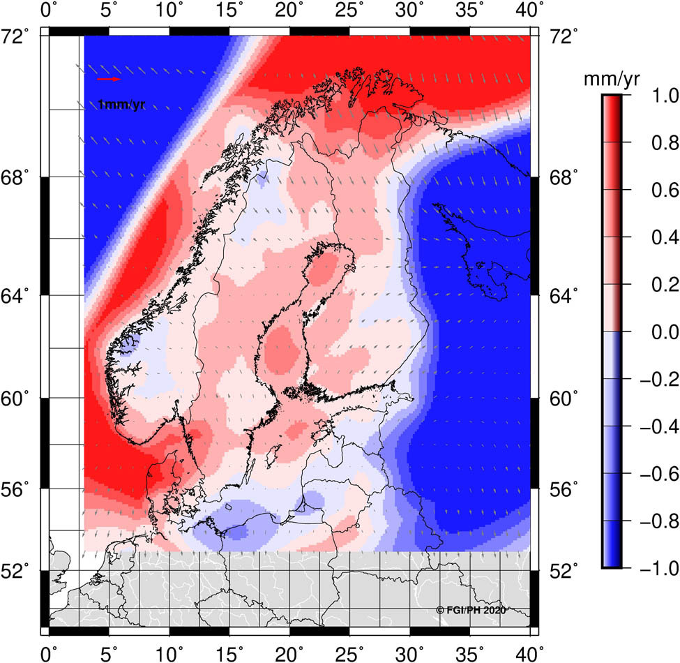
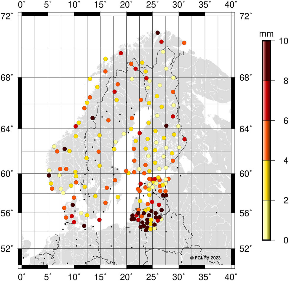
In the NKG2020 transformation, we use the latest NKG land uplift (or deformation) model NKG_RF17vel (Figure 2). It is a 2D + 1D model where the vertical and horizontal velocities were estimated separately. Vertical velocities equal to those of the NKG2016LU_abs model described in Vestøl et al. (2019). Horizontal velocities were developed later with a similar methodology, and the final 2D + 1D model was released at the beginning of 2020.

NKG_RF17vel model intraplate velocities. Black vectors denote horizontal velocities in ETRF2014. Vertical velocities shown with the colormap. Unit: mm/year.
The NKG2016LU model is based on data from repeated precise leveling, GNSS time series (Kierulf et al. 2021), and GIA model that were combined with least-squares collocation (LSC). The horizontal velocities are based on the GNSS time series (Lahtinen et al. 2019; Kierulf et al. 2021), and the GIA model (Häkli et al. 2019) that were combined with a similar LSC approach. Minor, but unfortunate effect of the separate modeling is that the vertical velocities are aligned to IGb08 (Rebischung 2012) whereas the horizontal velocities are aligned to ETRF2014 (via IGb14). The systematic difference between vertical IGb08 and IGb14 velocities was estimated to be approximately 0.1 mm/year which was considered insignificant compared to the uncertainties. This, along with the fact that the NKG2016LU model had been released and was already in use, led to the conclusion not to alter the model due to this insignificant difference. This would have possibly caused more confusion. Furthermore, Häkli et al. (2016) discussed, thoroughly, why IGb08 (ITRF2008) is not suitable for the NKG transformation, and therefore, the horizontal velocities could not be transformed either. Hence, we consider the vertical velocities to be aligned to ITRF2014 within their uncertainties. Since the velocity difference is systematic, it did not affect the transformation residuals (they are adjusted to agree with the NKG_RF17vel model), but it may become visible with the future data sets (see also uncertainty discussion in Section 5).
The NKG_RF17vel model is a major improvement over the NKG_RF03vel model (Nørbech et al. 2006; Lidberg et al. 2007) that was used for the NKG2008 transformation. The biggest differences are the underlying station velocities and their uncertainties (the GNSS time series were extended from 1996–2004 to 1997–2017), improved GIA models, and enhanced combination strategy for horizontal velocities (from Helmert fit to LSC). Altogether, these improve the quality of the model but also the quantity of stations enabled a better selection of GNSS stations. The overall accuracy of the final NKG_RF17vel velocities was estimated as 0.1, 0.1, and 0.4 mm/year for North, East, and Up components, respectively. The final documentation of the NKG_RF17vel model is yet pending.
4 Results
In this section, we present the main results of the NKG2020 transformation. Most important are the national transformations (Helmert parameters and XYZ-grid in Figure 1). Furthermore, we have created a new transformation hub that can be used in applications spreading over two or more Nordic–Baltic countries. We present also the differences compared to the previously used NKG2008 transformation.
4.1 National transformation parameters and residuals
We derived the first coordinate set for estimating the national transformation parameters by applying equations (2) and (3) for the ITRF2014 coordinates described in Section 3.2. This yielded coordinates in ETRF2014 at epoch 2000.0, which is the common transformation hub for all countries and was labeled as NKG_ETRF14 (Section 4.3). We derived the second coordinate set from the national ETRS89 coordinates with reversed equation (5). From these coordinate sets, we estimated the national parameters with the seven-parameter Helmert transformation using equation (9), except for Norway where we ended up using a correction grid instead of the Helmert transformation (see next section). We estimated the national transformation residuals with equation (10), and they are plotted in (Figure 3). The residuals describe how well the two coordinate sets agree with each other at the transformation reference epoch 2000.0 and give an estimate of the expected transformation accuracy.
National residuals in 3D at the transformation reference epoch (2000.0). For the Norwegian case, values refer to coordinate differences between transformed and official national coordinates.
In most cases, the residuals are at a few millimeter levels (Table 2) proving that the Helmert transformation is still adequate for most countries. Larger residuals in Latvia can be explained by the early ETRS89 realization based on the EUREF‐BAL’92 campaign in 1992 with an estimated accuracy of a couple of centimeters. Latvia is underway to update the old LKS-92 realization with a new LKS-20 realization, and the parameters will be updated accordingly. Lithuanian residuals are larger than in the other countries. The horizontal residuals are rather good but in vertical some unexplained discrepancies remained. These will be investigated in the future. The final transformation parameters are given Table 3.
Rms of transformation residuals (NEU)
| rms | n | N (mm) | E (mm) | U (mm) |
|---|---|---|---|---|
| DK | 10 | 0.42 | 0.46 | 1.82 |
| EE | 23 | 1.85 | 2.18 | 2.36 |
| FI | 12 | 1.53 | 1.77 | 2.63 |
| LT | 31 | 3.54 | 3.22 | 12.60 |
| LV | 7 | 1.38 | 3.11 | 6.09 |
| NO* | 189 (35) | 0.7 (2.83) | 0.7 (2.09) | 2.7 (5.70) |
| SE | 69 | 0.87 | 0.70 | 2.12 |
| Total** | 179 | 1.86 | 1.82 | 3.33 |
*Norwegian transformation is based on correction grid, and therefore has no Helmert residuals. Here rms refers to coordinate differences between transformed NKG Repro1 and official ETRS89 coordinates (in brackets values from the initial Helmert transformation). ** Total used only for overall uncertainty estimation in Section 5 and for this consistency purposes some outliers were rejected.
National transformation parameters
| Country | #pts | m 0 (mm) | T X (m) | T Y (m) | T Z (m) | D (ppb) | R X (mas) | R Y (mas) | R Z (mas) |
|---|---|---|---|---|---|---|---|---|---|
| Denmark | 10 | 1.27 | 0.66818 | 0.04453 | −0.45049 | −3.136 | 3.12883 | −23.73423 | 4.42969 |
| Estonia | 23 | 2.26 | −0.05027 | −0.11595 | 0.03012 | 3.191 | −3.10814 | 4.57237 | 4.72406 |
| Finland | 12 | 2.26 | 0.15651 | −0.10993 | −0.10935 | 5.290 | −3.12861 | −3.78935 | 4.03512 |
| Latvia | 7 | 4.93 | 0.09745 | −0.69388 | 0.52901 | −49.663 | −19.20690 | 10.43272 | 23.27169 |
| Lithuania | 31 | 8.09 | 0.36749 | 0.14351 | −0.18472 | −3.684 | 4.79140 | −10.27566 | 2.76102 |
| Norway* | 189 | N/A (grid) | |||||||
| Sweden | 69 | 1.41 | 0.03054 | 0.04606 | −0.07944 | 3.002 | 1.41958 | 0.15132 | 1.50337 |
Rotations according to the IERS conventions (Petit and Luzum 2010). *In Norway a correction grid is used instead of the Helmert transformation.
4.2 Correction grid for Norway
Initially, we estimated the Helmert parameters with a subset of Norwegian CORS stations similar to the other countries (NKG Repro1 solution includes only the most stable stations). Already the residuals for the subset revealed some inconsistencies. To evaluate the performance for the rest of the CORS network, we used another extended data set with ITRF2014 coordinates at epoch 2020.0 for 189 CORS stations and transformed the coordinates with the defined parameters. The accuracy (rms) was 2.5, 7.7, and 6.7 mm for North, East, and up components, respectively, and extreme values being more than 2 cm (Table 4). These were considered too large. We estimated also modified Helmert parameters with all 189 stations, but they gave only slightly better results.
Residuals/coordinate differences for the pure Helmert parameters (defined with a subset of CORS stations) and for the correction grid
| Helmert | Correction grid | |||||
|---|---|---|---|---|---|---|
| n = 189 | E (mm) | N (mm) | H (mm) | E (mm) | N (mm) | H (mm) |
| Min | −3.4 | −15.0 | −15.8 | −2.6 | −2.0 | −8.2 |
| Max | 5.6 | 4.7 | 23.2 | 1.9 | 3.3 | 8.8 |
| Mean | 1.5 | −6.2 | −0.4 | 0.0 | 0.0 | 0.4 |
| Stdev | 2.0 | 4.6 | 6.7 | 0.7 | 0.7 | 2.7 |
| rms | 2.5 | 7.7 | 6.7 | 0.7 | 0.7 | 2.7 |
Therefore, a method that corrects for weaknesses in the coordinates of the CORS network was needed. We used the gridding (LSC) method that was described in Section 2.2, and we estimated the final corrections as geocentric translations in a final three-dimensional grid. We used all 189 CORS stations with known ITRF2014 and national ETRS89 coordinates to develop the correction grid. We derived the input coordinates for LSC in the same way as described in the previous section yielding coordinates aligned to ETRF2014 at epoch 2000.0 and ETRF93 at epoch 2000.0. We applied LSC to the differences between these coordinates. We chose the LSC parameters based on tuning the signal and the noise. For the final grid, we used the observation variance C 0 = 0.0008 m2, the observation noise n = 0.025 m, and the correlation length D = 150 km.
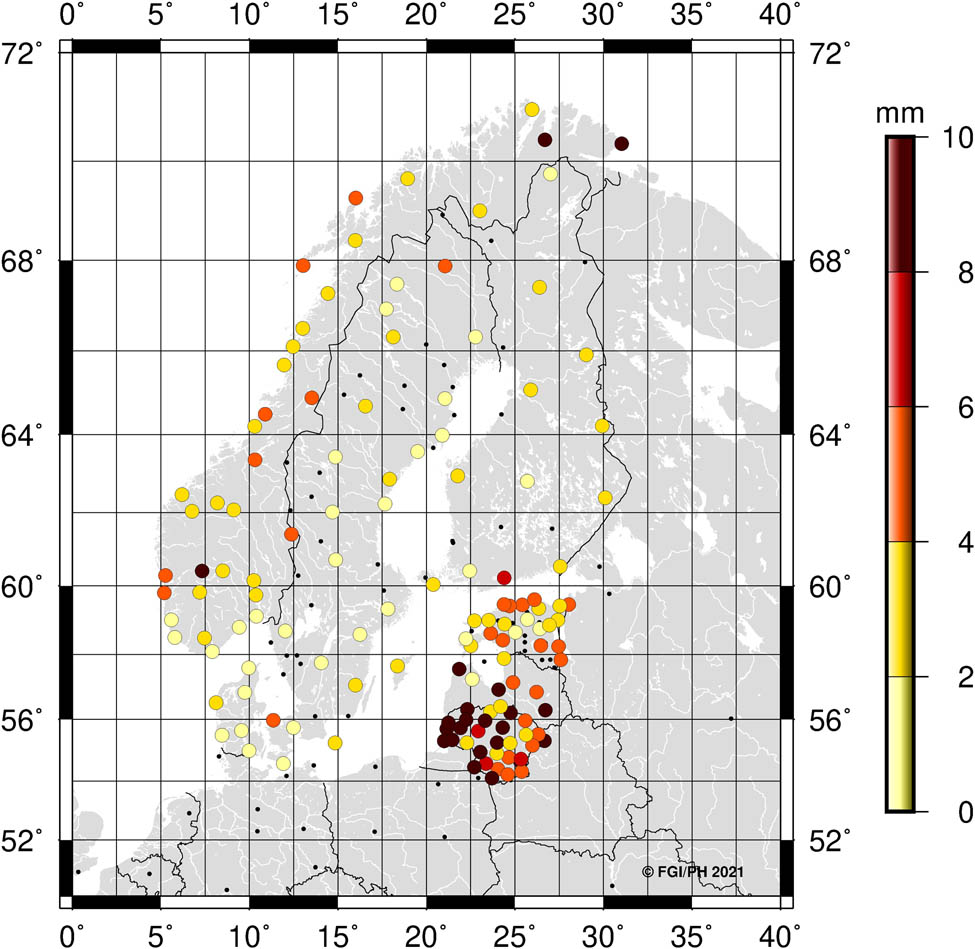
The accuracy (rms) with the grid improved to 0.7, 0.7, and 2.7 mm for North, East, and Up components, respectively, and the extreme values remained below 1 cm (Table 4). The first version of the LSC correction grid was released in PROJ version 8.0.1 on May 1, 2021 (Figure 4). The grid was updated with the second version of the grid in PROJ 9.0.1 on April 1, 2022. The correction grid was updated due to coordinate changes in some CORS stations in Northern Norway.

Norwegian correction grids in geocentric Cartesian X, Y, and Z coordinates.
The correction grid fulfills the preset expectations and has been easy to implement to the PROJ transformation library that enables easy access for the users.
4.3 Transformation hub
As a result of the NKG2020 transformation, we created a common reference frame aligned to ETRF2014. We labeled this reference frame as NKG_ETRF14. The main purpose of NKG_ETRF14 is to act as a transformation hub but the solution can also be used for pan-Nordic–Baltic or other applications that extend over two or more countries. One important example is the fitting of Nordic–Baltic gravimetric geoid models to GNSS-levelling data sets that should be in consistent reference frames. Therefore, we evaluated its consistency with the official ETRF2014 solutions provided by EUREF. EUREF releases reference frame solutions in ETRF2014 and updates them regularly with cumulative solutions (Legrand 2022b).
We analyzed NKG_ETRF14 with the latest (at the time of writing) solution called EPN_ETRF2014_C2220 covering GNSS data up to GPS week 2220 (Legrand 2022a). We propagated the EPN ETRF2014 coordinates from the frame reference epoch to that of the NKG_ETRF14, i.e., 2000.0 using the published station velocities in ETRF2014. The differences between NKG_ETRF14 and EPN_C2220 coordinates for common stations are shown in Figure 5 and summarized in Table 5.
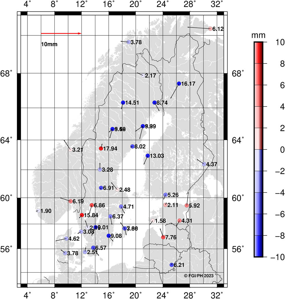
NKG_ETRF14 minus EPNC2220 (ETRF2014@2000.0).
Differences between NKG_ETRF14 and EPN_C2220 ETRF2014 coordinates at epoch 2000.0
| n = 41 | N | E | U |
|---|---|---|---|
| Min | −3.70 | −5.70 | −15.60 |
| Max | 3.30 | 1.40 | 17.90 |
| Mean | −0.35 | −0.75 | −2.61 |
| Stdev | 1.64 | 1.25 | 6.88 |
| rms | 1.67 | 1.46 | 7.36 |
| 95% | 3.25 | 2.70 | 15.69 |
Stations outside Nordic–Baltic countries excluded from the statistics.
The NKG_ETRF14 reference frame should not be used outside Nordic and Baltic countries. The reason is that the NKG_RF17vel model was aligned to ETRF2014 mostly with the data from the Nordic and Baltic countries and outside the coverage of geodetic data is worse, and the model is more dependent on the underlying GIA models. Therefore, we have excluded stations outside Nordic and Baltic countries from the Figure and Table. The results look mostly good but there are some larger differences that were not captured by the outlier analysis. They are likely to be caused by mismatching solution numbers and partly also by deviating station and model velocities. The overall agreement is 1.7, 1.5, and 7.4 mm for North, East, and Up components, respectively. Even without further outlier analysis, this proves that the NKG_ETRF14 is in good agreement with the official solutions.
4.4 Differences to the NKG2008 transformation
The previous version of the NKG transformation, the NKG2008 transformation, has been used in various applications, and therefore, it was important to evaluate the influences of updating to the new NKG2020 transformation. The differences in the transformation residuals at the transformation reference epoch 2000.0 are mostly small. These describe the consistency between new and previous data sets used for determining the parameters. The NKG2020 transformation is a major update over NKG2008. Considering the major improvements in the NKG2020, the differences in the residuals are surprisingly small.
However, the used intraplate velocity models differ significantly in some regions (Figure 6). In the Nordic and Baltic countries, the velocity differences remain at a few tenths of millimeter-per-year level for horizontal and up to a millimeter-per-year level for vertical velocities. These lead to differences in the transformed coordinates, and these differences are time-dependent. We took the NKG Repro1 solution and propagated the IGb14 coordinates to different epochs with the associated station velocities and then transformed these coordinates with both transformations. The results, indeed, show that the differences between the transformed coordinates are growing with time (two different epochs are shown in Figure 7). At the transformation reference epoch 2000.0, the differences are small unless the national coordinates have been updated between the NKG2008 and the NKG2020 transformations (which affect the transformation parameters). The difference does not explicitly tell which one has better accuracy, but in the next section, we show that the difference should be understood as an improvement.
NKG_RF17vel minus NKG_RF03vel_ETRF2000 (used in the NKG2008 transformation). NKG_RF03vel_ETRF2000 model was transformed to ETRF2014 before comparison to account for reference frame differences. Horizontal differences shown with grey vector and vertical differences with color map.

NKG2020 minus NKG2008 at transformation reference epoch 2000.0 (left) and at epoch 2020.0 (right). Horizontal differences shown with grey vector and vertical differences with color map.
5 Uncertainty estimation
The NKG transformation can serve as a tool to monitor or even maintain national reference frames, hence setting high demands on the accuracy (or more precisely uncertainty). The uncertainty estimates should be realistic over time. As described in Section 2.3, we estimate the uncertainty empirically and divide it into a constant and a time-dependent part. The transformation residuals were discussed in the Section 4.1, and here, we extend the uncertainties to cover other data sets as well.
5.1 Constant part
For the constant part, we extended the uncertainties from the residuals by using three independent data sets having ITRF2014 and ITRF2020 coordinates at the same epoch from which the NKG2020 transformation was determined, 2015.0. The redundant data sets give a more realistic picture of the NKG2020 transformation accuracy.
As the main solution, we used the NKG_Repro1_upd2020 solution (Lahtinen et al. 2022), which we considered the most dense, homogeneous, and up-to-date solution. It also consists of the stations that were regarded to be the most stable ones and suitable for geodynamical studies. As additional data sets, we used the EPN cumulative solution C2220 (Legrand 2022a) and the ITRF2020 solution by IERS (IGN 2023). The NKG and EPN solutions are aligned to IGb14 and the IERS solution to ITRF2020. We propagated all coordinates to epoch 2015.0 with the station velocities, transformed them with the NKG2020 transformation, and compared the resulting coordinates to the official national ETRS89 coordinates (Table 6).
NKG Repro1 upd2020: IGb14@2015.0, EPN_IGb14_C2220: IGb14@2015.0 and ITRF2020@2015.0 transformed to national ETRS89 realizations. rms of coordinate differences
| rms | NKG Repro1 upd2020: IGb14@2015.0 | EPN_IGb14_C2220: IGb14@2015.0 | ITRF2020@2015.0 | |||||||||
|---|---|---|---|---|---|---|---|---|---|---|---|---|
| Country | n | N [mm] | E [mm] | U [mm] | n | N [mm] | E [mm] | U [mm] | n | N [mm] | E [mm] | U [mm] |
| DK | 10 | 0.84 | 1.94 | 5.45 | 3 | 0.51 | 1.71 | 3.21 | 5 | 1.19 | 2.06 | 2.77 |
| EE | 25 | 1.89 | 2.10 | 2.10 | 4 | 3.01 | 2.93 | 2.54 | 1 | 2.50 | 2.50 | 0.00 |
| FI | 46 | 1.05 | 1.34 | 3.53 | 19 | 0.64 | 0.40 | 1.36 | 3 | 1.18 | 1.09 | 2.81 |
| LV | 6 | 0.96 | 3.29 | 2.38 | ||||||||
| LT | 29 | 3.56 | 4.21 | 9.39 | ||||||||
| NO* | 35 | 2.01 | 1.39 | 3.35 | 5 | 2.49 | 2.87 | 2.59 | 6 | 2.88 | 2.75 | 3.30 |
| SE | 67 | 1.17 | 1.18 | 2.67 | 30 | 1.26 | 1.44 | 2.49 | 21 | 1.39 | 1.19 | 3.26 |
| Total | 222 | 1.69 | 1.78 | 3.59 | 64 | 1.47 | 1.59 | 2.41 | 39 | 1.79 | 1.84 | 3.31 |
*Norway with correction grid.
Especially, the ITRF2020 solution has much fewer stations than the NKG solution in the Nordic and Baltic region; yet the overall coordinate differences (rms) between different solutions agree with each other horizontally within a few tenths of millimeters and vertically within approximately one millimeter. On one hand, the good agreement proves that the NKG2020 transformation performs well with different data sets. On the other hand, the results suggest that also ITRF2020 coordinates can also be transformed with the same accuracy-level as ITRF2014 coordinates. The sample was rather small but still the results indicate that the transformation works as planned and that it can be used for ITRF2020 coordinates without further modifications. We tested the recently released IGS20 solution (Villiger 2022) with the NKG2020 transformation as well, but the solution includes even fewer common stations for comparison. Hence, the results are not shown here but also they indicate similar accuracy as with the ITRF2020 solution.
The coordinate differences in Table 6 are the same within a few tenths of a millimeter compared to the residuals of the NKG2020 transformation (cf. Table 2). Hence, the additional component for the total uncertainty budget is negligible for the used GNSS solutions. However, this additional uncertainty component is directly proportional to the used input data and our values reflect the high quality of the GNSS solutions.
The initial results indicated that the differences include most likely some outliers due to, e.g., mismatches in solution numbers between the ITRF and the ETRS89 coordinates (offsets due to instrument changes; Section 5.2). Here, the results refer to the latest solution number in the ITRF solutions, but most likely not all national coordinates agree with this selection. However, checking all solution numbers would have required a thorough and laborious analysis and was disregarded. Instead, we applied a simple outlier detection with three-sigma rejection criteria to the results and considered this to fit the purpose. Differences from the NKG_Repro1_upd2020 solution are shown in Figure 8.
NKG_Repro1_upd2020@2015.0 transformed to the national ETRS89 realizations and compared to the official national ETRS89 coordinates. 3D coordinate differences shown in the plot.
5.2 Time-dependent part
We used daily coordinate time series from the cumulative NKG Repro1 upd2020 solution to evaluate the time-dependent part of the NKG2020 transformation. Cumulative solutions are typically available with regular intervals and can be used to account for, e.g., instrument changes or tectonic events in contrast to infrequently updated reference frame solutions. Typically, station coordinates and velocities with their uncertainties are provided as the result of a reference frame solution, and daily coordinate time series preceding the time series analysis may not be available. In our case, we had the NKG Repro1 upd2020 daily coordinate time series at our disposal. The advantage of daily coordinate time series is that all available data can be used for analysis, e.g. regarding the length of time series and the number of stations. Some stations may have been rejected from secular reference frame solutions if regarded as too unstable. Moreover, daily coordinate time series gives a more detailed picture of the station behavior (e.g., seasonal signals) than just a linear velocity. A disadvantage is that one has to perform the time series analysis oneself to extract, e.g., linear or residual velocities and their uncertainties.
We transformed the daily IGb14 coordinates with the NKG2020 transformation and compared them to the official ETRS89 national coordinates. We analyzed the residual time series in the national ETRS89 realizations with the Hector software (Bos et al. 2013). The data set was the same as for the NKG Repro1 upd2020 reference frame solution release and was therefore already cleaned from outliers and had pre-defined epochs for offsets too. Time series span from 3.3 to 23.5 years, average being almost 13 years. The number of solutions varies from 1–6 (offsets from zero to five), the average being 2. While being a tectonically rather silent region, except for the land uplift, we estimated the magnitudes of the offsets and one linear trend for the whole data period (secular velocity) as well as annual signals. For the estimation of velocity uncertainties, we used a combination of power-law noise plus white noise models.
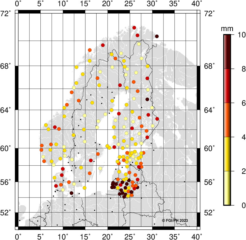
The NKG2020 transformation accounts for the rigid plate motions and land uplift effects, and therefore, the residual velocities are optimally close to zero. The remaining non-zero velocities indicate either uncertainties in the NKG_RF17vel deformation model or uncertainties or some local effects in the station velocities. The residual velocities with the estimated uncertainties are shown in Figure 9.

Residual velocities in the national ETRS89 realizations (mm/year). Residual velocities in horizontal shown with black vectors and their uncertainties with error ellipses. Vertical residual velocities shown with colored circles and their uncertainties with vertical bars.
Most of the residual velocities are close to zero but quite many larger velocities exist. To analyze possible reasons, we show the length of the time series as well as a number of solutions (offsets) in the time series in Figure 10. Already this explains that most of the larger residual velocities are attributed to shorter time series (smallest circles in the figure). However, some larger vertical velocities are related to long time series as well. Many of these cases are related to discrete time series. Therefore, increasing number of offsets has a clear effect on the residual velocities. The NKG_RF17vel model is based on least-squares collocation that smooths the station velocity field considering the velocity uncertainties, and the aim is to describe the small-scale land uplift phenomenon. Therefore, non-zero residual velocities are most likely caused by the station time series that are either inaccurate or describe some local phenomena. For further analysis, we plotted the ratio of observations and solution numbers in Figure 11. This reflects the length of the uninterrupted time series. Now, most of the larger residual velocities are clearly attributed to the short uninterrupted time series. A couple of exceptions of long uninterrupted time series (large circles) with slightly larger vertical residual velocities pop up: KUUS and ARJ0. Both stations are affected by accumulating snow on the antenna radome every winter. The effect is treated slightly differently in the NKG Repro1 upd2020 (Lahtinen et al. 2022) and BIFROST2015 solutions (Kierulf et al. 2021). Latter was used to develop the NKG2016LU model (the vertical part of the NKG_RF17vel model) and thus included in the NKG2020 transformation. Also, the time spans and the processing setups are different, and altogether, these may explain 0.3–0.4 mm/year vertical residual velocities we observe. On the other hand, the figure shows that the discrete time series do not always result in bad velocities.

Same as Figure 9 but the circle sizes showing the lengths of time series (larger circle means longer time series). Time series vary between 3.3 and 23.5 years. Number of offsets (by means of solution numbers) in the time series shown as a number beside the circle for stations with more than two solution numbers.
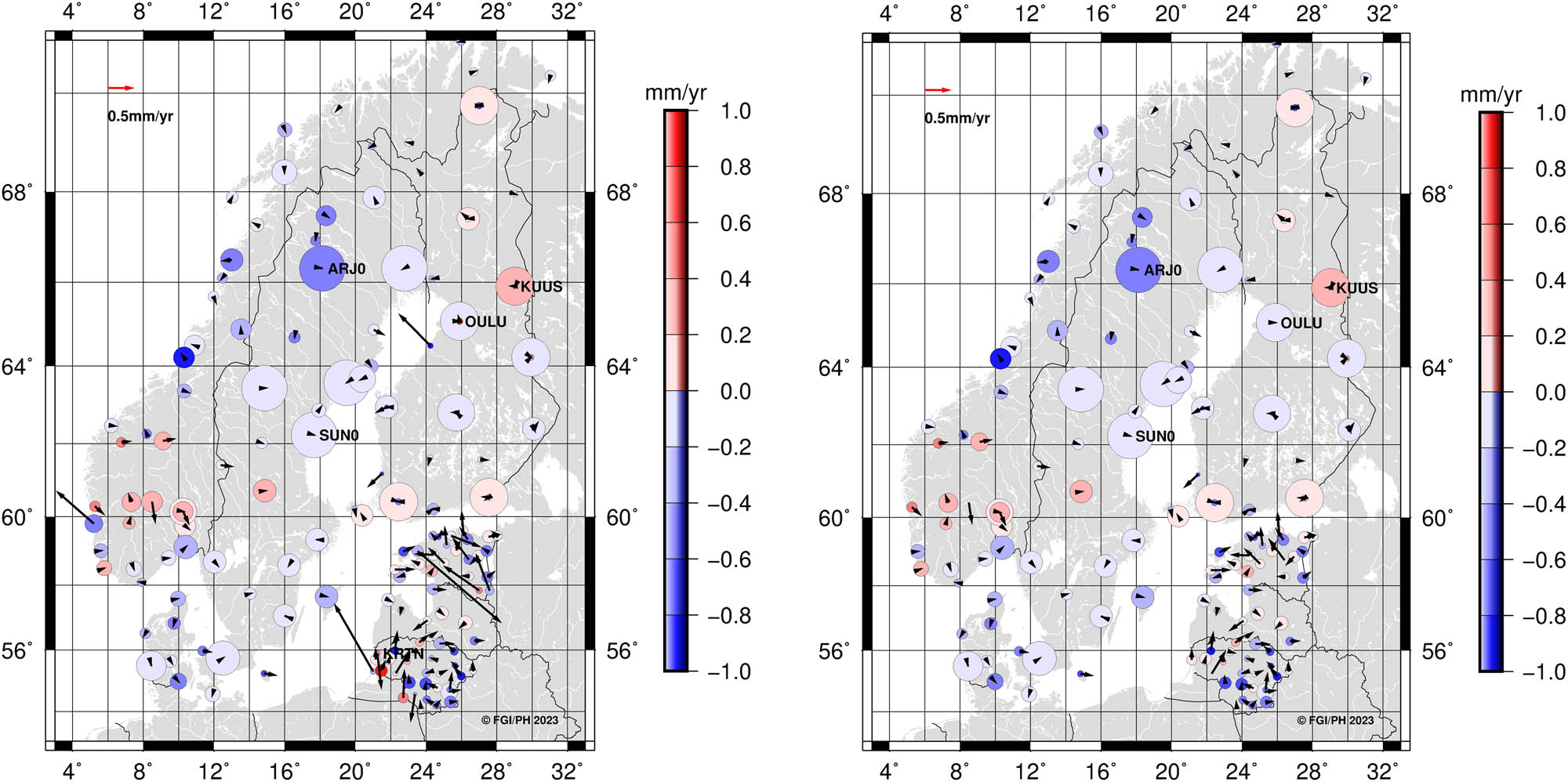
Same as Figure 9 but the circle sizes show the ratio of observations and offsets (number of observations divided by the number of solutions). Results before outlier analysis on the left-hand side and after on the right-hand side. This describes the length of the uninterrupted time series. Increasing number of offsets affects the quality of time series.
Considering these ambiguities in the residual velocity analysis, it is difficult to give one definite answer to the transformation accuracy over time. However, the longest time series and/or longest uninterrupted time series suggest that the transformation is almost time-invariant see example from SUN0 station in Figure 12. At the other end, the residual velocities are dominated by inaccuracies and local effects in station velocities, see the examples from KRTN station in Figure 13 and OULU/OUL2 twin station in Figure 14. Somewhere between these ends, the uncertainties of the model and station velocities are converging to describe the actual time-variable accuracy for our purpose.
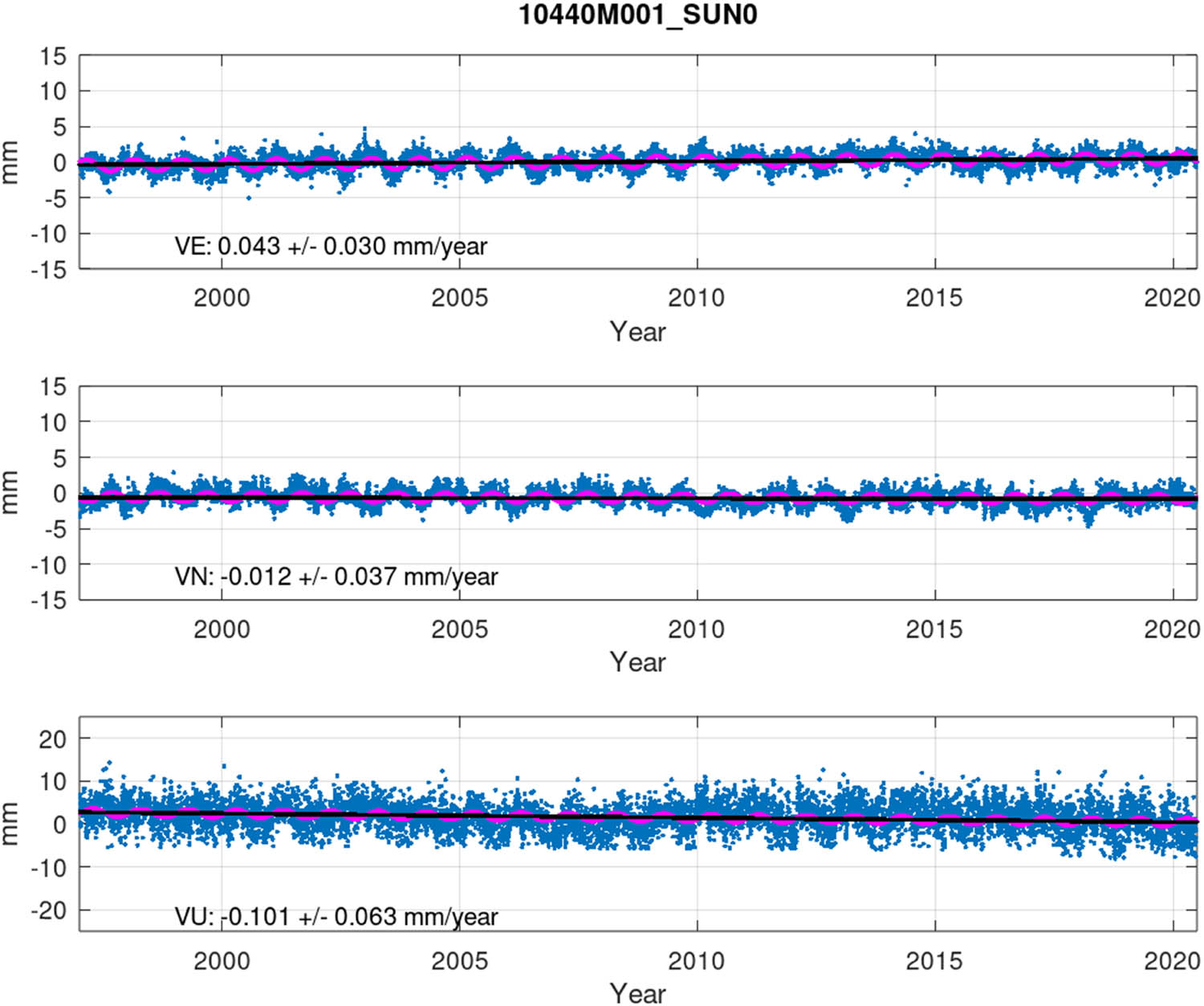
Example of the residual time series and velocities for SUN0 station in Sweden.
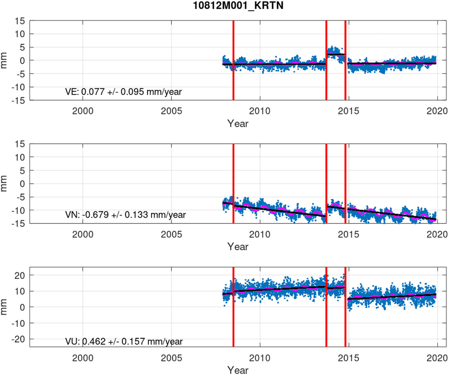
Example of the residual time series and velocities for KRTN station in Lithuania. Several offsets in the time series cause jumps in the coordinates but there are also significant remaining trends in the time series. The station was used for determining the NKG2020 transformation parameters but was found too unstable to be included in the NKG_RF17vel modeling and was captured also in our outlier analysis. Therefore, the residual velocities likely describe local effects.
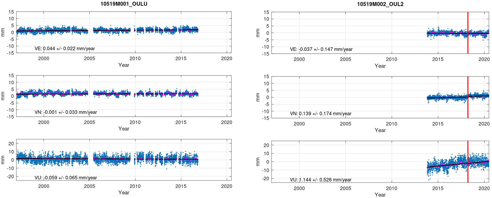
Example of twin stations OULU and OUL2. The stations are located only 25 meters from each other, so in principle, the residual velocities should converge. The results show large differences in the residual velocities that are likely to be caused by, e.g., deviating time spans in the time series. OUL2 was rejected in the outlier analysis.
Table 7 summarizes the results for 148 time series. To derive statistics, we performed a simple outlier analysis (three-sigma criteria; Figure 11). Based on the analysis, we could reject most of the deviating stations (e.g., KRTN and OUL2 were captured in the outlier analysis). On average, the residual velocities are very close to zero suggesting well-aligned model velocities. We consider the rms in Table 7 as the best estimate for the time-dependent part of the NKG2020 transformation uncertainty and conclude that it is 0.1, 0.1, and 0.3 mm/year in North, East, and Up components, respectively. The extreme residual velocities are in the order of one millimeter per year.
Statistics of the residual velocities in the national ETRS89 realizations. Outlier detection performed
| n = 148 | N (mm/year) | E (mm/year) | U (mm/year) |
|---|---|---|---|
| Min | −0.42 | −0.37 | −1.02 |
| Max | 0.44 | 0.39 | 0.58 |
| Mean | 0.02 | 0.01 | −0.16 |
| Stdev | 0.12 | 0.13 | 0.30 |
| rms | 0.12 | 0.13 | 0.34 |
| 95% | 0.30 | 0.27 | 0.72 |
Combining the constant and time-dependent parts from the NKG_Repro1_upd2020 solution, we conclude that the empirically estimated overall accuracy of the NKG2020 transformation is 1.7 mm ± 0.1 mm/year, 1.8 mm ± 0.1 mm/year, and 3.6 mm ± 0.3 mm/year in North, East, and Up components, respectively (1σ). The constant part is given at epoch 2015.0. These values suggest a few millimeter of stability over 10 years that can be considered a very good result.
5.3 Accuracy today (@2023.0)
Even though we derived the overall accuracy (covering constant and time-dependent parts), we evaluated the accuracy also empirically at a recent epoch 2023.0 from a multiyear secular reference frame solution. This is a common way to process ITRF coordinates, and therefore, we get another estimate for the actual accuracy. Similarly to Section 5.1, we used the NKG Repro1 upd2020 solution, propagated the coordinates to epoch 2023.0, transformed them with NKG2020 transformation, and compared the transformed coordinates to the official ETRS89 coordinates. The results are shown in Figure 15 and Table 8. The results show that the estimated total uncertainty with constant and time-dependent parts is quite conservative and that the reference frame solution seems to absorb a part of the uncertainties. Some differences can be caused by different analysis methods like data rejections, noise models, etc. In the end, this again is one more proof that the NKG2020 transformation performs well.
Accuracy today (simple outlier detection applied). IGb14@2023.0 transformed to the national ETRS89 realizations and compared to the official national ETRS89 coordinates.
NKG Repro1 upd2020: IGb14@2023.0 transformed to the national ETRS89 realizations and compared to the official national ETRS89 coordinates
| Country | n | N [mm] | E [mm] | U [mm] |
|---|---|---|---|---|
| DK | 10 | 1.14 | 2.25 | 5.98 |
| EE | 24 | 2.57 | 2.73 | 3.26 |
| FI | 47 | 0.95 | 1.05 | 3.74 |
| LV | 6 | 1.28 | 4.00 | 4.45 |
| LT | 29 | 4.12 | 4.33 | 11.72 |
| NO | 35 | 2.03 | 1.42 | 4.57 |
| SE | 67 | 1.26 | 1.55 | 3.21 |
| Total | 222 | 1.85 | 2.08 | 4.42 |
rms of coordinate differences.
6 Conclusions and discussion
We presented an update to the NKG transformation and labeled it as the NKG2020 transformation. The NKG2020 transformation follows the previously defined methodology but is a major update consisting of fully revised and improved data. We also improved the uncertainty estimation.
6.1 Technical solution
We showed that the accuracy of the NKG2020 transformation is at the level of a few millimeters at the transformation reference epoch (residuals) in most cases. We extended the uncertainty estimate from residuals by using three independent data sets and found similar accuracies to the residuals. The improved deformation model NKG_RF17vel, as a part of the NKG2020 transformation, was shown to be able to produce almost static coordinates over time for the most stable reference stations. Overall, we found the empirical accuracy (uncertainty at epoch 2015.0): 1.7 mm ± 0.1 mm/year, 1.8 mm ± 0.1 mm/year, and 3.6 mm ± 0.3 mm/year in North, East, and Up components, respectively (1σ).
As a result, the accuracy degrades only a few millimeters in 10 years. It was also shown to operate equally with the recently released ITRF2020. Therefore, the NKG2020 transformation can be used as a long-term solution without immediate needs for updates. However, such needs may arise from updates in the national reference frames.
The NKG2020 transformation supersedes the previous version NKG2008 due to updated national realizations in many countries. Several improvements over the NKG2008 make NKG2020 more accurate, especially regarding the time-dependency. In many countries, the difference between the NKG2020 and NKG2008 transformations is almost zero at the transformation reference epoch 2000.0 but the differences are growing in time due to different deformation models.
As a new method, we presented a correction grid for the national transformations as a part of the NKG2020 transformation. Such a grid was developed and applied to Norwegian transformation and was shown to correct some deficiencies in regular Helmert transformation, thus improving the accuracy of the national transformation. Correction grid method gained interest also from other countries, but for the moment all countries except Norway still rely on national Helmert transformations.
6.2 Role of the NKG2020 transformation
The NKG2020 transformation is intended as a technical solution to harmonize the transformations from global ITRF coordinates to the national ETRS89 realizations in the Nordic and Baltic countries. As a collaborative work, it already has an official status in many countries, but this should always be confirmed by the appropriate national authority if needed. As a technical solution, the NKG2020 transformation offers an accurate link between global and national coordinates. As such it also provides an option for maintaining static national reference frames under the influence of crustal motions.
Nordic and Baltic reference frames, by means of static coordinates, get deformed over time due to the land uplift. Locally, in (traditional) relative surveying the deformations are normally insignificant but more and more geospatial solutions are relying on nationwide or even global positioning services. Nationwide networks may not be fixed (accurately) directly to the national ETRS89 realizations due to too large deformations. On the other hand, society and GIS systems need static coordinates that do not vary in time. We are also in the advent of global positioning services becoming in wider use. Such services typically provide coordinates in global dynamic reference frames.
The NKG2020 transformation provides a tool to keep the geospatial registries in the national ETRS89 realization and perform positioning in an accurate global dynamic reference frame. This is referred to as a two-frame approach or sometimes to as a semi-dynamic datum (or preferably reference frame). As an example, Finland has deployed the NKG2020 transformation for determining the highest order coordinates (“realization”) of the national EUREF-FIN reference frame. The NKG2020 transformation is used to define coordinates for lower-order active stations as well and for monitoring (maintenance) of the EUREF-FIN.
6.3 Access and standardization of reference frames and transformations
Globalization in the geospatial data domain means the analysis of data from different sources. At the same time, demands for accuracy are increasing. In many places, technical solutions exist (like the NKG2020 transformation) but the standardization is still lagging or is under development. Therefore, it is crucial to develop standardization for reference frames and transformations to ensure seamless and errorless data analysis without misinterpretations.
Several international geodetic registries have been developed to improve standardization regarding reference frames and transformations. Registries store the data including the methods and parameters defining geodetic reference systems and adopted transformations between them. This common information is available for various applications in the geosciences, such as GIS software decreasing the need for customized solutions thus ensuring more homogeneous results. One of the most popular geodetic registries is the EPSG registry (IOGP 2023). NKG joins the standardization work with plans to register the NKG2020 transformation to the EPSG registry. EPSG codes facilitate the use of coordinate reference systems and transformations and decrease risks for mistakes, e.g., in reference frame or transformation-related information. Also, submission to the ISO geodetic registry (ISO 2023) has been in consideration.
In addition to geodetic registries, some open geodetic code libraries exist. One widely used library for coordinate transformations is the PROJ software package for coordinate transformations (Evenden et al. 2022). PROJ is used by several GIS software and implementations, thus serving as a standardization for coordinate transformations. A reference implementation of the NKG2020 transformations was provided in the PROJ software package from version 8.1.0 and onwards. The implementation is compatible with the ISO 19111:2019 standard (ISO 2019) and the EPSG registry. At the time of writing, the transformations have not yet been submitted to the IOGP for inclusion in the EPSG registry but with the PROJ implementation in place, the necessary data modeling is in place.
A prerequisite for such libraries and software is proper data licenses. The NKG2020 transformation and associated data (e.g., NKG_RF17vel model) are attributed to the CC-BY4.0 license (CC 2023) to give wide permissions of use.
The initial goal of the NKG transformations was to harmonize the data and transformations. The PROJ implementation and open data licenses make the NKG2020 transformation and associated data widely available to users.
6.4 Future work
In the short term, we are planning to register NKG2020 in the EPSG registry. This facilitates the use of the transformations and makes them even more accessible. Latvia is about to update its national ETRS89 realization, and associated parameters will be calculated and released as soon as the realization will come into force. Other updates will be made when necessary.
In the longer term, NKG has plans for updating several fundamental data sets related to the NKG transformation. These include reprocessing of an extended (both spatially and temporally) GNSS solution aligned to the latest ITRF2020 reference frame. The velocity field with realistic uncertainty estimates together with an improved GIA model will serve as the basis for an updated deformation model. With the new deformation model also a new version of the NKG transformation becomes rational (NKG 2022).
Acknowledgements
We thank all the members of the NKG Working Group of Reference Frames and all Nordic and Baltic representatives who contributed and made this important work possible. We also acknowledge the other NKG working groups; without successful collaborative work, the necessary data would not be in place. We are grateful to anonymous reviewers for improving the manuscript.
-
Conflict of interest: Authors state no conflict of interest.
-
Data availability statement: The NKG2020 transformation is available in PROJ transformation software: https://proj.org/.
References
Altamimi, Z. 2018. EUREF Technical Note 1: Relationship and Transformation between the International and the European Terrestrial Reference Systems. http://etrs89.ensg.ign.fr/pub/EUREF-TN-1.pdf [Accessed 2 February 2023].Search in Google Scholar
Altamimi, Z., P. Rebischung, L. Métivier, and X. Collilieux. 2016. “ITRF2014: A new release of the International Terrestrial Reference Frame modeling nonlinear station motions: ITRF2014.” Journal of Geophysical Research: Solid Earth 121(8), 6109–31. 10.1002/2016JB013098.Search in Google Scholar
Borre, K. and P. Petroskevicius. 1995. “Fundamental GPS network in Lithuania, Geodetic Theory Today.” In: Third Hotine-Marussi Symposium on Mathematical Geodesy, L’Aquila, Italy, May 30–June 3, 1994. p. 27–31. Springer.10.1007/978-3-642-79824-5_8Search in Google Scholar
Bos, M. S., R. M. S. Fernandes, S. D. P. Williams, and L. Bastos. 2013. “Fast error analysis of continuous GNSS observations with missing data.” Journal of Geodesy 87(4), 351–60. 10.1007/s00190-012-0605-0.Search in Google Scholar
CC, 2023. Creative Commons Attribution 4.0 International (CC BY 4.0). [online] https://creativecommons.org/licenses/by/4.0/. [Accessed 3 February 2023].Search in Google Scholar
Crook, C., N. Donnelly, J. Beavan, and C. Pearson. 2016. “From geophysics to geodetic datum: updating the NZGD2000 deformation model.” New Zealand Journal of Geology and Geophysics 59(1), 22–32. 10.1080/00288306.2015.1100641.Search in Google Scholar
Decree of Geodetic System. [online] https://www.riigiteataja.ee/akt/128102011003?leiaKehtiv. [Accessed 5 February 2023].Search in Google Scholar
Donnelly, N., C. Crook, R. Stanaway, C. Roberts, C. Rizos, and J. Haasdyk. 2015. “A two-frame national geospatial reference system accounting for geodynamics.” REFAG 2014, International Association of Geodesy Symposia, edited by van Dam T., p. 235–42, Cham: Springer International Publishing. 10.1007/1345_2015_188.Search in Google Scholar
Evenden, GI., E. Rouault, F. Warmerdam, K. Evers, T. Knudsen, H. Butler, et al. 2022. PROJ. [online] Zenodo. 10.5281/ZENODO.6646503.Search in Google Scholar
Fankhauser, S. and W. Gurtner. 1995. “EUREF-DK94 Denmark Euref Densification Campaign.” Satelliten-Beobachtungsstation Zimmerwald. Universität Bern.Search in Google Scholar
Häkli, P., S. Lahtinen, U. Kallio, and H. Koivula. 2021. Update of EUREF-FIN. [online] https://www.nordicgeodeticcommission.com/wp-content/uploads/2021/04/NKG_WGRF2021_1-2_Hakli_Update_of_EUREF-FIN.pdf [Accessed 3 February 2023].Search in Google Scholar
Häkli, P., M. Lidberg, L. Jivall, T. Nørbech, O. Tangen, M. Weber, et al. 2016. “The NKG2008 GPS campaign – final transformation results and a new common Nordic reference frame.” Journal of Geodetic Science 6(1), 1–33. 10.1515/jogs-2016-0001.Search in Google Scholar
Häkli, P., M. Lidberg, L. Jivall, H. Steffen, H. P. Kierulf, J. Ågren, et al. 2019. “New horizontal intraplate velocity model for Nordic and Baltic countries.” In: FIG Working Week 2019. [online] Geospatial information for a smarter life and environmental resilience. Hanoi, Vietnam: FIG. https://www.fig.net/resources/proceedings/fig_proceedings/fig2019/papers/ts01e/TS01E_haekli_lidberg_et_al_10078.pdf> [Accessed 2 February 2023].Search in Google Scholar
IERS. 2023. The International Terrestrial Reference Frame (ITRF). [online] https://www.iers.org/IERS/EN/DataProducts/ITRF/itrf.html [Accessed 12 May 2023].Search in Google Scholar
IGN. 2023. ITRF2020. [online] https://itrf.ign.fr/en/solutions/ITRF2020 [Accessed 3 February 2023].Search in Google Scholar
IOGP. 2023. EPSG Geodetic Parameter Dataset. [online] https://epsg.org/home.html [Accessed 3 February 2023].Search in Google Scholar
ISO. 2019. ISO 19111:2019 Geographic Information — Referencing by Coordinates.Search in Google Scholar
ISO. 2023. ISO Geodetic Registry (ISOGR). [online] https://geodetic.isotc211.org/ [Accessed 13 May 2023].Search in Google Scholar
Jivall, L., P. Häkli, P. Pihlak, and O. Tangen. 2010. “Processing of the NKG 2008 campaign.” In: Proceedings of the 16th General Assembly of the Nordic Geodetic Commission. p. 143–9. Sundvolden, Norway: Norwegian Mapping Authority.Search in Google Scholar
Jivall, L., J. Kaminskis, and E. Paršeliūnas. 2007. “Improvement and extension of ETRS 89 in Latvia and Lithuania based on the NKG 2003 GPS campaign.” Geodezija ir kartografija 33(1), 13–20. 10.1080/13921541.2007.9636710.Search in Google Scholar
Jivall, L. and M. Lidberg. 2000. “SWEREF 99 – an updated EUREF realisation for Sweden.” In: Report on the Symposium of the IAG Subcomission for Europe (EUREF), EUREF. p. 167–75. Publication. [online] Tromsø, Norway. http://www.euref.eu/symposia/book2000/P_167_175.pdf.Search in Google Scholar
Jivall, L. and C. Lilje. 2023. Review and update of SWEREF 99 in 2021. Lantmäterirapport.Search in Google Scholar
Kierulf, H. P., H. Steffen, V. R. Barletta, M. Lidberg, J. Johansson, O. Kristiansen, et al. 2021. “A GNSS velocity field for geophysical applications in Fennoscandia.” Journal of Geodynamics 146, 101845. 10.1016/j.jog.2021.101845.Search in Google Scholar
Kierulf, H. P., G. Valsson, K. Evers, M. Lidberg, P. Häkli, D. Prizginiene, et al. 2019. “Towards a Dynamic reference frame in Iceland.” Geophysica 54(1), 3–17.Search in Google Scholar
Kollo, K., J. Metsar, P. Pihlak, and A. Ellmann. 2019. Computation of the Estonian GNSS permanent station network and its submission as EUREF densification. Tallinn, Estonia: Estonian Land Board.Search in Google Scholar
Kosenko, K. 2022. LATREF stations coordinates estimation - LKS-20. [online] https://www.nordicgeodeticcommission.com/wp-content/uploads/2022/06/NKG_WGRF2022_1-1_Kosenko.pdf [Accessed 3 February 2023].Search in Google Scholar
Kristiansen, O. and B. G. Harsson. 1999. “The new norwegian national geodetic network EUREF 89.” In: Proceedings of the General Assembly of the Nordic Geodetic Commission 25–29 May, 1998, LMV-rapport. p. 162–95.Search in Google Scholar
Lahtinen, S., L. Jivall, P. Häkli, T. Kall, K. Kollo, K. Kosenko, et al., 2019. “Densification of the ITRF2014 position and velocity solution in the Nordic and Baltic countries.” GPS Solutions 23(4), 95. 10.1007/s10291-019-0886-3.Search in Google Scholar
Lahtinen, S., L. Jivall, P. Häkli, and M. Nordman. 2022. “Updated GNSS velocity solution in the Nordic and Baltic countries with a semi-automatic offset detection method.” GPS Solutions 26(1), 9. 10.1007/s10291-021-01194-z.Search in Google Scholar
Legrand, J. 2022a. EPN Multi-year Position and Velocity Solution C2220. Royal observatory of Belgium (ROB). 10.24414/ROB-EUREF-C2220.Search in Google Scholar
Legrand, J. 2022b. EPN Multi-year Position and Velocity Solutions. Royal observatory of Belgium (ROB). 10.24414/ROB-EUREF-CWWWW.Search in Google Scholar
Lidberg, M., J. M. Johansson, H.-G. Scherneck, and J. L. Davis. 2007. “An improved and extended GPS-derived 3D velocity field of the glacial isostatic adjustment (GIA) in Fennoscandia.” Journal of Geodesy 81(3), 213–30. 10.1007/s00190-006-0102-4.Search in Google Scholar
Madsen, F. and B. Madsen. 1993. “A New GPS-network in the Baltic Countries.” In: Report on the Symposium of the IAG Subcommission for the European Reference Frame (EUREF). Budapest, Hungary: Verlag der Bayerischen Akademie der Wissenschaften in Kommission bei der C.H.Beck’schen Verlagsbuchhandlung. p. 83–91.Search in Google Scholar
Metsar, J., K. Kollo and A. Ellmann. 2018. “Modernization Of The Estonian National Gnss Reference Station Network.” Geodesy and Cartography 44(2), 55–62. 10.3846/gac.2018.2023.Search in Google Scholar
Metsar, J., K. Kollo, A. Ellmann, A. Rüdja, and P. Pihlak. 2019. “Multi-epoch GNSS campaigns of the national geodetic network in Estonia.” Geophysica 54(1), 51–60.Search in Google Scholar
Moritz, H. 1980. Advanced physical geodesy. Sammlung Wichmann: Neue Folge: Buchreihe; Bd. 13. Karlsruhe: Tunbridge, Eng: Wichmann; Abacus Press.Search in Google Scholar
NGS, 2021. Blueprint for the Modernized NSRS, Part 1: Geometric Coordinates and Terrestrial Reference Frames. NOAA Technical Report NOS NGS. [Technical Report] Silver Spring, MD: National Oceanic and Atmospheric Administration. https://geodesy.noaa.gov/library/pdfs/NOAA_TR_NOS_NGS_0062.pdf [Accessed 2 February 2023].Search in Google Scholar
NKG, 2022. NKG structure 2022-2026. [online] https://www.nordicgeodeticcommission.com/wp-content/uploads/2022/09/NKG-structure-2022-2026_final.pdf [Accessed 3 February 2023].Search in Google Scholar
NKG, 2023. Nordic Geodetic Commission. [online] https://www.nordicgeodeticcommission.com/ [Accessed 3 February 2023].Search in Google Scholar
Nørbech, T., K. Engsager, L. Jivall, P. Knudsen, H. Koivula, M. Lidberg, et al. 2006. ”Transformation from a Common Nordic Reference Frame to ETRS89 in Denmark, Finland, Norway, and Sweden – status report.” In: Proceedings of the 15th General Meeting of the Nordic Geodetic Commission, Technical Report. p. 68–75. Copenhagen, Denmark: DTU Space.Search in Google Scholar
Ollikainen, M., H. Koivula, and M. Poutanen. 1999. “The densification of the EUREF Network in Finland.” In: Report on the Symposium of the IAG Subcommission for Europe (EUREF). p. 114–22. Prague, Czech Republic: EUREF Publication.Search in Google Scholar
Ollikainen, M., H. Koivula, and M. Poutanen. 2000. The densification of the EUREF network in Finland. Suomen Geodeettisen Laitoksen julkaisuja. [online] Kirkkonummi. http://hdl.handle.net/10138/346606.Search in Google Scholar
Paršeliūnas, E. and A. Būga. 1995. “GPS activities, coordinate systems, geoid determination in Lithuania.” Reports of the Finnish Geodetic Institute. p. 17–30. Helsinki: Finnish Geodetic Institute.Search in Google Scholar
Petit, G. and B. Luzum. 2010. IERS Conventions. IERS Technical Note. p. 179. [online] Frankfurt am Main: Verlag des Bundesamts für Kartographie und Geodäsie. https://www.iers.org/IERS/EN/Publications/TechnicalNotes/tn36.html. [Accessed 3 February 2023].Search in Google Scholar
Rebischung, P. 2012. [IGSMAIL-6663] IGb08: an update on IGS08. https://lists.igs.org/pipermail/igsmail/2012/000497.html [Accessed 4 February 2023].Search in Google Scholar
Rebischung, P. 2020. [IGSMAIL-7921] Switch to IGb14 reference frame. https://lists.igs.org/pipermail/igsmail/2020/007917.html [Accessed 4 February 2023].Search in Google Scholar
Rüdja, A. 1999. “A new ETRS89 system for Estonia.” In: Report on the Symposium of the IAG Subcommission for the European Reference Frame (EUREF). p. 123–36. EUREF Publication. Prague, Czech Republic: Veröff. Bayr. Komm. Intern. Erdmessung.Search in Google Scholar
Valsson, G. 2021. “Surveying in the land of fire and ice.” GIM International 35(7), 18–21.Search in Google Scholar
Vestøl, O. 2006. “Determination of postglacial land uplift in Fennoscandia from leveling, Tide-gauges and continuous GPS stations using least squares collocation.” Journal of Geodesy 80(5), 248–58. 10.1007/s00190-006-0063-7.Search in Google Scholar
Vestøl, O., J. Ågren, H. Steffen, H. Kierulf, and L. Tarasov. 2019. “NKG2016LU: a new land uplift model for Fennoscandia and the Baltic Region.” Journal of Geodesy 93(9), 1759–79. 10.1007/s00190-019-01280-8.Search in Google Scholar
Villiger, A. 2022. [IGSMAIL-8238] Upcoming switch to IGS20/igs20.atx and repro3 standards. https://lists.igs.org/pipermail/igsmail/2022/008234.html [Accessed 3 February 2023].Search in Google Scholar
© 2023 the author(s), published by De Gruyter
This work is licensed under the Creative Commons Attribution 4.0 International License.
Articles in the same Issue
- Research Articles
- Two adjustments of the second levelling of Finland by using nonconventional weights
- A gap-filling algorithm selection strategy for GRACE and GRACE Follow-On time series based on hydrological signal characteristics of the individual river basins
- On the connection of the Ecuadorian Vertical Datum to the IHRS
- Accurate computation of geoid-quasigeoid separation in mountainous region – A case study in Colorado with full extension to the experimental geoid region
- A detailed quasigeoid model of the Hong Kong territories computed by applying a finite-element method of solving the oblique derivative boundary-value problem
- Metrica – An application for collecting and navigating to geodetic control network points. Part II: Practical verification
- Global Geopotential Models assessment in Ecuador based on geoid heights and geopotential values
- Review Articles
- Local orthometric height based on a combination of GPS-derived ellipsoidal height and geoid model: A review paper
- Some mathematical assumptions for accurate transformation parameters between WGS84 and Nord Sahara geodetic systems
- Book Review
- Physical Geodesy by Martin Vermeer published by Aalto University Press 2020
- Special Issue: 2021 SIRGAS Symposium (Guest Editors: Dr. Maria Virginia Mackern) - Part II
- DinSAR coseismic deformation measurements of the Mw 8.3 Illapel earthquake (Chile)
- Special Issue: Nordic Geodetic Commission – NKG 2022 - Part I
- NKG2020 transformation: An updated transformation between dynamic and static reference frames in the Nordic and Baltic countries
- The three Swedish kings of geodesy – Speech at the NKG General Assembly dinner in 2022
- A first step towards a national realisation of the international height reference system in Sweden with a comparison to RH 2000
- Examining the performance of along-track multi-mission satellite altimetry – A case study for Sentinel-6
- Geodetic advances in Estonia 2018–2022