
On the connection of the Ecuadorian Vertical Datum to the IHRS
-
José L. Carrión
 ,
Sílvio R. Correia de Freitas
,
Sílvio R. Correia de Freitas

Abstract
In this work, the determination of the discrepancy between the Ecuadorian Vertical Datum (EVD) and the International Height Reference System (IHRS) is presented. The vertical offset was estimated at the EVD based on the fixed geodetic boundary value problem approach. The focus of the experiment was the determination of the anomalous potential in the EVD, which in turn enable determination of the respective geopotential value. Taking a geopotential space-based approach, two estimates of the EVD offset with respect to the IHRS were obtained that amount to −1.51 and −1.61 m2/s2.
1 Introduction
In view of the implications of geodetic reference frames for human activities, aiming at information consistency and interoperability at the global level, and recognizing the coordinated approach of International Association of Geodesy (IAG), the United Nations (UN) established oriented actions toward the global development of geospatial information. IAG through global geodetic observing system (GGOS) aims to achieve the geodetic infrastructure necessary for monitoring the Earth system and for supporting research on global changes, considering product requirements on a global scale. Thus, activities related to earth observation are the focus of GGOS, including monitoring and modeling of dynamic earth processes such as mass and angular momentum exchanges, mass transport and ocean circulation, and changes in sea, land, and ice surfaces (Plag et al. 2009). In studying regional and planetary phenomena, a unique physical vertical reference system is one of the key themes established by GGOS (Kutterer and Neilan 2015). These actions, developed in the context of the United Nations Global Geospatial Information Management, were embodied in UN Resolution A/RES/69/266 on 26th February 2015. The main objective was the brief description of the key elements of the Global Geodetic Reference Frame (GGRF) as the realization of the Global Geodetic Reference System (GGRS) according to the approaches followed under IAG’s coordination. Within the aforementioned structure, the fundamental role of GGRF the facilitation of the integration of different geometric and gravimetric observations with the central objective of providing reliable and high-quality products and services. Recent achievements related to GGRS/GGRF can be found in (SIRGAS 2019). In this framework, IAG Resolution #1 established in 2015 defines the equipotential surface of the gravity field with geopotential W 0 = 62636853.4 m2/s2 as the datum of the International Height Reference System (IHRS). The primary vertical coordinates of Pi points referred to this system are the geopotential numbers C Pi = W 0 − W Pi , from which the required physical height can be derived. This aspect is included as the GGOS Theme 1 – Unified Height System (IAG 2015). This Resolution has triggered a number of activities within the IAG’s scopes (Ihde et al. 2017). In 2016, the IAG established the GGRS structures as the ideal junction of the International Terrestrial Reference System with the IHRS (IAG 2016), so that its realization (GGRF) is linked to the International Terrestrial Reference Frame (ITRF) with International Height Reference Frame (IHRF) stations. It should be noted that the IHRF is now at the stage of establishing procedures and conventions (IAG 2019). These activities are supported by Working Group 0.1.2 on strategies for the realization of the IHRS, established in February 2016 and triggering activities in September 2016, within the scope of GGOS Theme 1. Nowadays, the activities related to IHRS/F are embodied in the Resolution #3/2019 from IAG which states that the International Gravity Field Service (IGFS) is responsible for the coordination of the activities. As already pointed out, this geodetic infrastructure can be used in the analysis and study of temporal evolution of several physical phenomena in the Earth’s system (GGOS 2016). Furthermore, IHRS allows compatibility of the physical vertical component with valuable information from space technologies such as global navigation satellite system (GNSS), Doppler orbitography and radiopositioning integrated by satellite, Very long baseline integrated by Satellite, satellite laser ranging, Gravity Recovery and Climate Experiment (GRACE), Gravity Field and Steady State Ocean Circulation Explorer, and several satellite altimetry missions. The establishment of the IHRF presupposes knowledge of the discrepancies between the local vertical datums (LVDs) in relation to a global reference surface. These discrepancies can amount to a maximum absolute value of about 2 m due to the mean dynamic ocean topography (MDOT) (Heck and Rummel 1990). Each LVD is referred to a particular equipotential surface (W 0i ) associated with the MDOT in a given tide gauge at a given epoch. Thus, in general, the W 0i values are not coincident with the global IHRS conventional value W 0 (Bosch 2002). Considering the aspects mentioned above, a fundamental task today is to achieve the link between the National vertical reference systems (NVRSs) and IHRS. In the case of South and Central America, SIRGAS (Geocentric Reference System for the Americas, IAG Sub-Commission 1.3b), with its Working Group III (SIRGAS-WG-III), is also seeking to implement a strategy for the establishment of a unified vertical reference system based on the integration of the NVRSs with the IHRS (De Freitas 2015). According to GGOS concepts, and to achieve SIRGAS’s goal of unification of Vertical Datums (VDs) in South America, classical VDs have to adapt to the IHRS, defined in terms of the geopotential. Thus, the modernization of the classical VDs, involves the computation of the discrepancies between each LVD potential value (W 0i ) and the IHRS potential value (W 0) as follows:
A unique global reference, determined by an equipotential surface of the gravity field W 0, and materialized with respect to a level ellipsoid, opens the possibility of the determination of globally unified physical heights (Rummel 2012). The approach to this problem has several facets, among which we can mention: the clear definition of the reference levels of each vertical network considered associated with the reference epoch of its corresponding VD; its current relation with the IHRS; the evolution of mean sea level (MSL) based on time series of observations with GNSS, tide gauges, and satellite altimetry; local discrepancies deduced from gravimetry associated with leveling and heights from the global positioning technique; ocean–continent integration from oceanic gravimetry contiguous to the VD, ocean gravity models, digital elevation models (DEMs), and geometrical models of the sea surface height. A gravimetric geoid model for Ecuador has not yet been calculated, because there is not enough gravimetric information for this purpose. However, regional models based on GNSS/leveling records have been generated (Carrión 2013; Leiva 2014; Tierra and Acurio 2017).
Carrión and De Freitas (2016) explored the adherence of GGMs in relation to the Ecuadorian Vertical Reference System heights, and furthermore estimated their offset in relation to a global reference surface based on MGGs (GO_CONS_GCF_2_TIM_R5 and EGM2008). Also, a first approximation to the estimation of the geopotential in the Ecuadorian Vertical Datum (EVD) was carried out by Carrión et al. (2018), considering the free solution of the geodesy boundary value problem (GBVP).
The central topic of this work is the determination of the discrepancy between the EVD and the IHRS, in the form as δW i /γ i , where γ i is the gravity at the VD under consideration, and δW i corresponds to the offset between the LVD and IHRS in terms of geopotential. As such, the offset was modeled at the EVD on the fixed GBVP solution. The Remove–Compute–Restore technique was adopted as a strategy for estimating the gravitational potential (Sansò and Sideris 2013). Global geopotential models (GGMs) were considered in order to model the long and very long wavelengths of the gravity field (from 2 to 360 degrees of harmonic series, according to Schwarz (1984)). The DEM was used to apply the residual terrain model (RTM) technique for modeling the short and very short wavelengths of the gravity field (from 361 to 36,000 degrees of harmonic series, according to Schwarz (1984)). Least squares collocation (LSC) was then applied for estimating the residual component of the anomalous potential. In situ gravimetric observations from different sources were used in the computations. Several terrestrial and aerial gravimetric databases were integrated for the continental part and complemented with gravimetric information derived from altimeter satellites and shipborne gravimetry on the oceanic area. Geopotential modeling was performed in the region under study which is centered at La Libertad – Ecuador tide gauge. Thus, the estimate of the discrepancy between the EVD and IHRS was essentially obtained as a geopotential value.
2 Materials and methods
2.1 Additional remarks about HRS
According to IAG Resolution #1 – 2015, the definition of the IHRS is given in terms of geopotential parameters, the vertical coordinates being geopotential numbers referred to an equipotential surface of the earth’s gravity field realized by a global conventional value W 0, computed as detailed in Sánchez et al. (2016). The establishment of the IHRS meets the requirements of GGOS, which according to its terms of reference must: (1) support a precise (at centimetric level) combination of physical and geometric heights on a global scale; (2) enable the unification of existing LVDs; and (3) guarantee vertical coordinates with global consistency (the same accuracy everywhere) and long-term stability (the same order of accuracy at all times) (Sánchez and Sideris 2017). The realization of the IHRS must be carried out in terms of geopotential values and be established according to well documented conventions. The coordinates in the IHRF are the geopotential numbers: the transformation of the geopotential numbers into physical heights and the geometric link to the reference surface are a matter of the IHRF realization and not of definition. As already pointed out, in order to establish the IHRS, it is necessary to adopt a conventional W 0, estimate the local values W 0i , and determine their differences according to equation (1) (Ihde et al. 2010).
2.2 Fixed GBVP
Potential boundary value problems (BVPs) are applied in physical geodesy to the determination of the gravitational potential V outside the earth masses (which is a harmonic function). If the densities within the planet and its boundary were known, the potential of the Earth’s gravitational field could be found through an integration over the total Earth’s volume υ (Torge and Müller 2012).
where G is the universal gravitational constant, ρ is the density of topographic masses, and l the distance to the mass element and the attracted point (Hofmann-Wellenhof and Moritz 2006).
However, the densities inside the earth are in general poorly known and this formula (equation (2)) cannot give an accurate estimate of the gravitational potential. So, usually, the external gravitational potential is obtained by means of the potential theory and considering the terrestrial surface as boundary. Several GBVPs, which are based on the BVPs of the potential theory, have been developed. As an example, one can consider the GBVP problem that is used in classical geoid determination, which is based on the knowledge of gravity anomalies Δg geoid = g geoid – γ ellipsoid (clearly dependent on reductions for the effect of the topographic masses above the geoid). Another very well-known GBVP is the Molodensky’s problem (Molodensky et al. 1962) which allows finding the solution without topographic reductions for the Earth’s crust gravity effect.
The Molodensky’s theory is the basis of the modern vision for solving the GBVP by applying the boundary condition on the physical surface of the earth related to the normal derivative of the so-called disturbing potential T (difference between the true earth’s gravity potential (W) and modeled theoretical ones (U)).
Since the publication of the basic works of Stokes (1849) and Molodensky et al. (1962), the determination of the external gravity field of the earth from gravity observations performed on the earth’s surface has been related to the solution of a free BVP of potential theory (Heck 2011).
The advent of accurate satellite positioning techniques (GNSS) and the consequent knowledge of earth’s surface geometry makes it possible to replace the free GBVP by the fixed one. Thus, the fixed GBVP solution is based on the determination of the geopotential W (x, y, z) in the space outside the terrestrial surface (Heck 2011). In the fixed solution, gravity disturbances (δg) are used instead of gravity anomalies (Δg), and are the input for the disturbing potential computation.
The terms in equation (4) are obtained by solving the Hotine’s integral as (Hotine 1969) follows:
where R is the mean earth’s radius and σ is the unit sphere. The term u i is associated with local corrections and criteria for linearization. Usually, the computation methods involve only the first two corrections given by equations (6) and (7) (Hofmann-Wellenhof and Moritz 2006).
where h and h
P are the heights of the integrating and computing points, respectively (referred to the ITRF2008, epoch 2016.43), and
The integral kernel H(Ψ) in equation (5) has the following form (Hofmann-Wellenhof and Moritz 2006):
where Ψ is the angular spherical distance between the computation and integration point.
2.3 Remove–compute–restore technique
According to Forsberg (1997), the remove–compute–restore technique allows a frequency analysis of the data. The long wavelength component of the data is modeled via a GGM. The gravimetric signal that dominates the short wavelengths of the gravity field, derived from the gravitational effect of the topographic masses, can be used to smooth the gravitational field before performing the modeling processes. The long and the short wavelength components are removed from the observed Q quantity by subtracting the corresponding terms (Q RTM, Q GGM) according to the below expression:
In this approach, the effect of topography on gravity (Q RTM) is obtained as the effect of the topographic masses in between the actual digital terrain model (DTM) and a mean long wavelength DTM surface corresponding to the maximum degree of the GGM used to compute the gravity effect of the long and very long wavelengths (Q GGM). This residual terrain effect in planar approximation (Forsberg and Tscherning 2008) can be expressed as follows:
where G is the universal gravitational constant, ρ is the standard density of the topographic masses, h P is the height of the computation point given by a DTM, z is the height relative to the reference surface, h ref is the mean long wavelength of DTM, [x P, y P, z P] are the computation point coordinates, and [x Q, y Q, z Q] are the integration point coordinates (Forsberg and Tscherning 1997).
On the other hand, the Q GGM quantity, corresponding to the long and medium wavelength of the gravity field, is computed from a GGM which is given as a truncated spherical harmonic series. The residual Q r component is then used in the “compute” step which can be based on, for e.g., LSC.
2.4 LSC and least squares fast collocation (LSFC)
The LSFC method, developed by Bottoni and Barzaghi (1993), is a variant of LSC, aimed at reducing computing time and required computational resources. The Fast Collocation method involves imposing constraints on input data. In case homogeneous and gridded data are considered, the covariance matrix has a particular structure that allows a fast computation of the collocation solution. If a two-dimensional data grid is considered and a covariance function that is only dependent on the plane distance d PQ between points P and Q
one can prove that the covariance matrix C computed for this grid using the covariance function of equation (12) is a symmetric block Toeplitz matrix and that each block has a Toeplitz structure. Given this highly regular structure, efficient algorithms for storing the matrix and for solving the collocation formula can be found.
2.5 Study region
The study has been carried out in a region centered on the EVD (Figure 1), more precisely in an area centered on BM03, i.e., the reference benchmark linked to the tide gauge named La Libertad. The study region is delimited by a square of 4° and having as centroid the EVD. The region between latitudes 0°13′10.1172″S–4°13′10.1172″S, and longitudes 78°54′19.4652″W−82°54′19.4652″W, is characterized by an irregular topography/bathymetry which ranges approximately from −4,698 to 1,552 m, involving the ocean – continent transition zone. The region shows high seismic activity, mainly due to the subduction of the Nazca Plate under the South American Plate; additionally, deformations of continental geological structures generate superficial earthquakes (Yepes et al. 1994). Historically, earthquakes of great magnitude have been recorded in Ecuador. The country is located in the Pacific “Circle of Fire,” the area with the largest seismic activity on the planet (Gonzales et al. 1988). Climatic phenomena are periodically related to the influence of ocean currents, among which we have the equatorial currents, Humboldt current, and the El Niño phenomena. These phenomena generally produce variations in temperature and, consequently, variations in the density of oceanic waters due to thermal expansion/contraction.
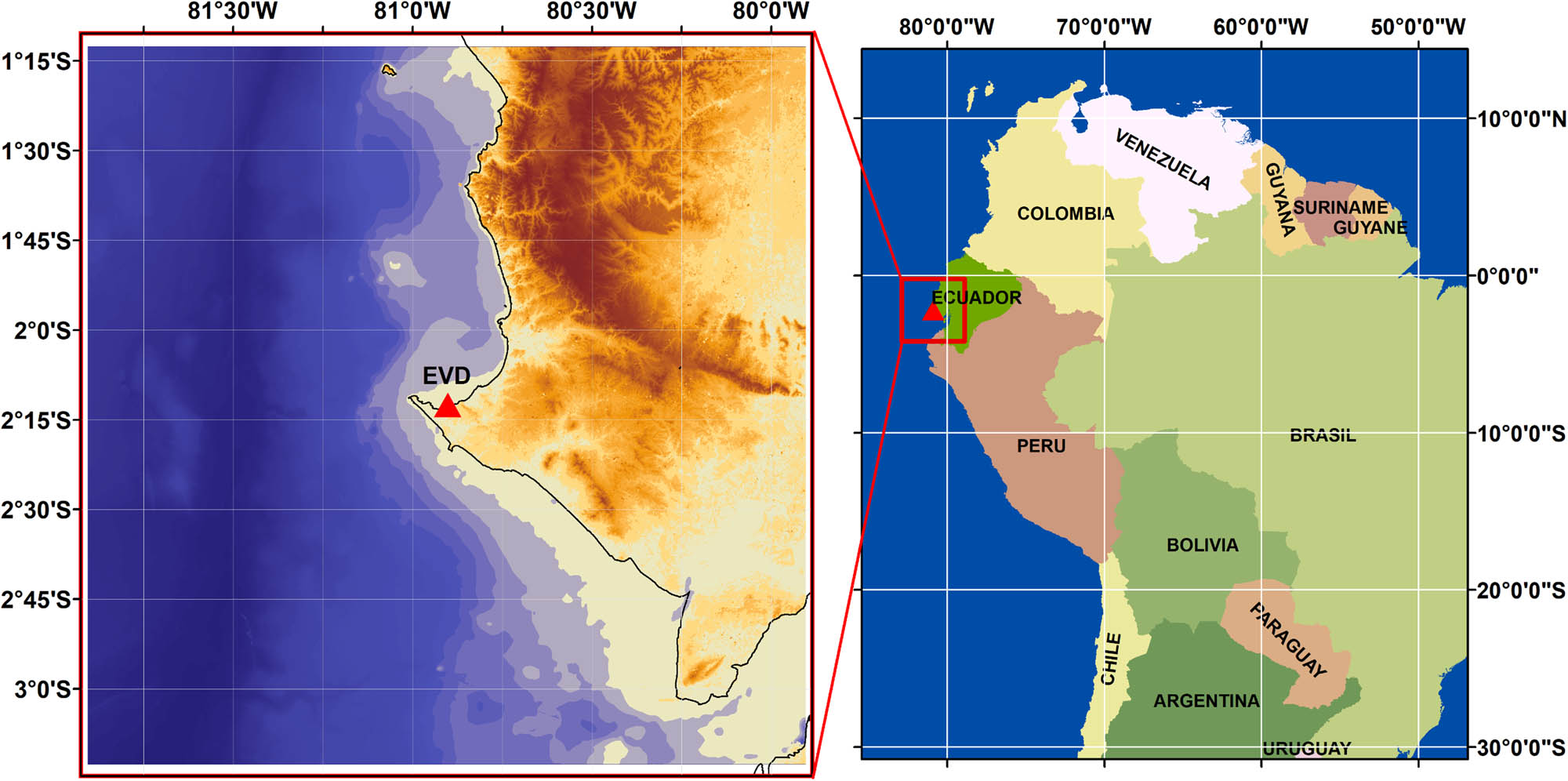
EVD location (La Libertad).
As said, the EVD discrepancy computation in relation to the IHRS was performed considering the BM03 benchmark (Figure 1) as the computation point. The coordinates of BM03 refer to the observation made by the Geographical Army Institute of Ecuador (IGM-EC) prior to the earthquake that occurred on 16th April 2016 and are in the SIRGAS 95 reference epoch 1995.4 (IGM-EC 2013). BM03 was affected by the aforementioned earthquake, the epicenter of which was located near the EVD, with magnitude 7.8 on the Richter seismological scale.
The computations developed in this study were performed considering the pre-seismic positions, and therefore, the displacement in the VD due to the seismic event must be considered for future computations and applications. We found the existence of several MSL determinations carried out by Ecuadorian Navy Oceanographic Institute (INOCAR) at the La Libertad tide gauge station since its installation. Also, according to INOCAR reports, BM48 is the origin point benchmark of the Ecuadorian Vertical Reference Network (EVRN). However, currently the EVRN origin point considered by the IGM-EC refers to the MSL value defined for the tide gauge observation period 1988–2009 and materialized in the BM03 benchmark.
2.6 Gravity dataset
Due to the non-availability of a unique and consistent geodetic database containing the information required for the development of this work, it was necessary to acquire gravity data from different sources. The diversity of data sources also implies the existence of records with heterogeneous characteristics, mainly in terms of observation methods and epochs, spatial distribution, associated precisions, and equipment used.
The main features of the geodetic data used in this work are detailed in the following. In total, 4,808 points with terrestrial gravimetric information (Figure 2b) were compiled within the region of 4° × 4° centered on the EDV point.

(a) Ocean gravity data from BGI database (black), and from SGGSA (red). (b) Terrestrial gravity data. (c) Airborne gravity records. (d) Gravity anomalies from WGM2012 model. (e) Gravity anomalies from DTU15 model.
In addition to the observed gravity, the records provide information about latitude, longitude, and leveled heights. Terrestrial gravity data records have been collected for geodetic purposes by the IGM-EC (Ecuadorian Military Geographic Institute) since the 1960s. In this group, gravity records were mostly observed on the principal highways mainly along with leveling lines. Some data refer to gravimetric densification campaigns. The ocean gravity data (3,209 records in black in Figure 2a) were made available by the Bureau Gravimétrique International (BGI) (2017). A smaller portion of the records located near the coast (321 records in red Figure 2a) was made available by the Subcommittee of Gravimetry and Geoid for South America (SGGSA) and refer to surveys for exploratory geophysics. The ocean gravity records of the BGI database, which are within the EVD contiguous region (4° × 4°), belong to 21 surveys carried out between 1957 and 1987. For each BGI record, the latitude, longitude, observed gravity, Free-Air anomaly, and Bouguer anomaly are known in the GRS67 (Geodetic Reference System 1967).
The airborne gravity records (3,443 points) contained in the 4° × 4° region in the vicinity of the EVD (Figure 2c) belong to the gravity data base of the SGGSA. The airborne gravity records are reduced to the terrain level according to WGS84 and EGM96 geoid, referred to the IGSN71 (International Gravity Standarization Net 1971) gravity datum and have information related to latitude, longitude, and height derived from a DEM. Gravity anomalies of the DTU15 model (Andersen and Knudsen 2016) derived from satellite altimetry (Figure 2e) and located in the oceanic part of the study region are also used as a source of complementary gravity information for modeling the earth’s gravity field. Finally, gravity values were also obtained from the World Gravity Map2012 (WGM2012) (Bonvalot et al. 2012). This is a set of maps of gravity anomalies and digital grids computed on a global scale based on gravity and height models. The WGM2012 model consists of a set of three maps of gravity anomalies (surface free-air anomalies, Bouguer anomalies, and isostatic anomalies) derived from the GGM EGM2008 and fill-in gravity information by the DEM ETOPO1. WGM2012 is the first set of maps of gravity anomalies that considers the contribution of most masses present on the surface of the planet (atmosphere, oceans, inland or continental seas, lakes, ice caps, etc.). The gravity anomalies of the WGM2012 model (Figure 2d) are obtained by rigorous computation, consistent with geodetic and geophysical definitions. The model provides homogeneous gravity information of the terrestrial gravity field on a regional and global scale. Since the gravimetric records come from different sources, it is necessary to consider their heterogeneity. According to Moritz (1980), LSC is a method that allows determining the anomalous gravity field by combining geodetic observations of different kinds (of different natures or with different spectral resolutions and precisions), through the efficient estimation of the gravitational field, by using the statistical characteristics of heterogeneous data in the form of covariance functions.
2.7 Gravity disturbance computation
Gravity disturbances were used in the computation in order to avoid local VD effects on geopotential modeling associated with reductions related to simplifying assumptions of the crust structure, in addition to the consideration of heights in local references. The processing performed on different data sources is detailed in the following sub-sections.
2.7.1 Gravity disturbances from records with no ellipsoidal height
In case of gravity records with no ellipsoidal height h, the values were approximated using the leveling heights H and N geoid undulations derived from the EIGEN6C4 GGM (N EIGEN6C4). This GGM presents the best performance in relation to other models in the assessment of geoidal heights in existing GNSS/lev data over Ecuador (2,972 records), with an average accuracy of 50 cm. For the continental records (4,808), this approximation was performed for 2,547 gravity points (52.97% of the continental gravity dataset). Thus, in such points, the estimated ellipsoidal heights were obtained as follows:
where H and N are the orthometric height and the geoid undulation, respectively.
Actually, H and N EIGEN6C4 are biased. H is biased since it refers to a given tide gauge and the Mean Sea Level is only approximatively coincident with the geoid. N EIGEN6C4 is, as well, biased since, in most of the cases, it has been estimated using ∆g which is computed by using H. However, in the context of the computation of the normal gravity value at ground level, which enters in the definition of δg, the use of equation (13) has a limited impact (we tested the misclosure in equation (13) on a set of values along the leveling lines finding a mean discrepancy of 0.252 m (Kirby 2003). As for the ocean gravity dataset (3,209 records), ellipsoidal heights are unknown for all the gravity records. Therefore, the values of h were approximated by mean sea surface (MSS) values derived from the DTU15 global marine gravity field model (Andersen and Knudsen 2016).
Finally, in the case of the airborne gravity dataset, ellipsoidal heights are available, and thus it was not necessary to compute approximate ellipsoidal heights. In the approximate computation of h (for terrestrial gravity data), N EIGEN6C4 (geoidal heights from EIGEN6C4 GGM) and H (leveling heights) referring to the zero-tide (ZT) system were used in the form h = H + N EIGEN6C4. For the ocean records, the MSS values of the DTU15 model, originally referred to the mean tide (MT) system (personal communication with Ole Andersen, DTU researcher, 2016), were transformed to the ZT system. On the other hand, the DTU15 MSS values are referred to the Topex/Poseidon ellipsoid. Therefore, a datum transformation was required for the Geodetic Reference System 1980 (GRS80) ellipsoid. Thus, the difference of the heights (δh), referring to both reference systems, was computed considering the parameters of the involved reference ellipsoids as follows (Renganathan 2010):
where h 1 and h 2 are the ellipsoidal heights referring the two involved reference ellipsoids. The parameters a 2, a 1 are, respectively, the semi-major axes of ellipsoid 2 and ellipsoid 1; and b 2, b 1 are, respectively, the semi-minor axes of ellipsoid 2 and ellipsoid 1. In order to compute the gravity disturbances according to the IAG recommendations (Ihde et al. 2017), the ellipsoidal height, of the gravity records for which it is known, was transformed from the tide-free system to the ZT system. The observed gravity data and the gravity disturbances from the global models (DTU15 and WGM2012) must also be transformed, according to equation (20), to the ZT system because they refer to the MT system. The computation of the gravity disturbances from the in situ gravity data (continental and ocean) was performed according to the following equation (Hinze et al. 2005):
where δg atm is the atmospheric correction for the observed gravity, γ is the normal gravity computed for the reference geodetic system GRS80, Δg H is the correction for the Honkasalo term and δg h is the height correction applied to compute the normal gravity at the physical surface (equation (17)).
2.7.2 Gravity disturbances from DTU15 and WGM2012 gravity anomalies
Gravimetric information derived from DTU15 (satellite altimetry) and WGM2012 models (Δg mod) is used to fill gaps in the oceanic region of the study area (Figure 2a). The free-air gravity anomalies from DTU15 and free-air surface gravity anomalies from WGM2012 are transformed into disturbances according to the expression that relates the gravity anomalies with the gravity disturbances considering the normal gravity gradient (Moritz 1980).
where Δg mod is the gravity anomalies from the models, and δg h is the height correction applied to the gravity anomalies to be transformed into disturbances. According to Heiskanen and Moritz (1985), δg h can be rigorously computed by the second-order approximation given by the following formula:
where a is the semi-major axis of the reference ellipsoid, f its corresponding flattening, γ e is the normal gravity at the equator, φ is the latitude of the calculation point, and m is given by the following equation:
where ω is the earth’s rotation angular velocity, b the semi-minor axis of the reference ellipsoid, and GM the geocentric gravitational constant. For the δg h computation, we considered the formula related to the GRS80 ellipsoid, resulting in Hinze’s expression (Hinze et al. 2005).
with h in meters and δg h in mGal.
The DTU15 and WGM2012 gravity anomalies were transformed into gravity disturbances according to equation (16) and the corresponding h with N (geoidal height) and ζ (height anomaly) were substituted in equation (17). For this calculation, approximate values for ζ and N were obtained from the GGM EIGEN6C4 considering its maximum expansion degree in spherical harmonics series (n = 2,190). The values of ζ EIGEN6C4 and N EIGEN6C4 were computed for the ZT system, and Δg DTU15 was also transformed to the ZT system. The transformation is performed according to the following equation proposed by Ekman (1989):
Therefore, the gravity disturbances (δg mod) resulting from equation (16) also correspond to the ZT system, thus following the recommendations given by the IAG on the context of the establishment of the IHRF (Ihde et al. 2017).
2.8 Outlier filtering
Elimination of the ocean and terrestrial gravity outliers was based on the comparison of the observed and modeled gravity disturbances. The EIGEN6C4 GGM (considering its maximum degree in spherical harmonics expansion, n = 2,190), which in the working area has an accuracy of approximately 5 cm (determined by comparison with GNSS/lev records), was used as the basis for outliers filtering. The effect of residual terrain modeling (RTM) (Forsberg 1984) on EIGEN6C4 reduced the gravity disturbances and was considered to improve outlier detection. Because the EIGEN6C4 information reproduced the long and very long wavelengths of the gravity field, to be comparable with the observed gravity disturbances, they must also include the contribution of the short wavelengths of the gravity field obtained by RTM. The reference DTM surface for the RTM computation was determined by smoothing the maximum resolution DEM (SRTM1 – spatial resolution of 1 arc sec (Farr et al. 2007)) by applying a low-pass filter. The low-pass filtering was performed by computing the moving average having a size which is defined through statistical analysis of the root mean square (RMS) of the residuals obtained for different versions of the smoothed DEM (Tziavos et al. 2009; Carrion et al. 2015). Once the best cap size (2′) is defined, outliers in the gravity dataset were selected by applying the three-sigma criterion (3σ) based on the δg res statistics.
where δg obs is the gravity disturbances obtained from the observed gravity records, δg EIGEN6C4 is the gravity disturbances derived from the EIGEN6C4, and δg RTM is the contribution of the residual topography on the gravity disturbances.
The elimination of outliers was performed independently for each data subset. Gravity disturbances used to compute residual gravity disturbances (δg res) are presented in Figure 3.

Gravity disturbances after elimination of outliers.
The statistics for the sets of gravity disturbances (δg) after outlier elimination, presented in Table 1, show the characteristics of the gravity disturbances for each of the gravity datasets.
Statistics of gravity disturbances after outlier elimination (mGal)
| Min | Max | Mean | σ | N | % | |
|---|---|---|---|---|---|---|
| Ground gravity | −123.89 | 282.27 | 30.70 | 70.50 | 4,720 | 1.83 |
| Airborne gravity | −47.09 | 195.33 | 72.26 | 48.25 | 3,422 | 0.58 |
| Ocean gravity | −148.46 | 83.09 | −5.03 | 51.37 | 3,199 | 0.31 |
| DTU15 | −141.38 | 167.40 | −11.38 | 49.05 | 1,390 | 0.22 |
| WGM2012 | −109.20 | 341.55 | 48.01 | 81.78 | 692 | 2.81 |
| Gravity dataset | −148.46 | 341.55 | 29.31 | 67.12 | 13,423 | 1.03 |
2.9 Residual gravity disturbances computation
Residual gravity disturbances (δg res) were computed considering the contribution of the GO_CONS_GCF_2_DIR_R5 GGM, and the related RTM. The δg GOCONS_GCF_2_DIR_R5 gravity disturbances (Bruinsma et al. 2013) were computed for their maximum spherical harmonic expansion (n = 300) and also considering truncation up to n = 200, after evaluating the performance of various combinations of GO_CONS_GCF_2_DIR_R5 (truncated versions) with the EGM2008 GGM. For both solutions, the zero-degree term was included in the computations, in order to consider the difference between the values employed by the GGM and reference ellipsoid for the geocentric gravitational constant GM (Hofmann-Wellenhof and Moritz 2006). The process followed for the computation of residual gravity disturbance values (δg res) is shown in the flowchart in Figure 4.

Residual gravity disturbances computation.
The maximum expansion degree used to compute the gravity disturbances in the truncated GGM was experimentally defined by analyzing the performance, in terms of height anomalies, of several combinations of GO_CONS_GCF_2_DIR_R5 (varying its maximum degree) with EGM2008 (with an average accuracy of 6 cm, estimated by evaluating geoidal heights in GNSS/level records).
Height anomalies from the combined models were compared with values derived from GNSS/lev records, and the combined GGMs performance was evaluated according to the RMS for the differences ζ GNSS/lev −ζ GGM.
In Figure 5, it can be seen that the combined GGM with better performance (RMS = 0.2459 m) corresponds to that established by considering

GO_CONS_GCF_2_DIR_R5/EGM2008 combinations performance.
The variation in the RMS as a function of the window radius used for the low-pass filter to generate the smoothed DEM, according to the method proposed by Carrion et al. (2015), implied by the GO_CONS_GCF_2_DIR_R5 model can be seen in Figure 6. The optimal RTM solutions (radius =
where δg is the gravity disturbances data collected in the study, δg GGM is the gravity disturbances from the GO_CONS_GCF_2_DIR_R5 GGM, and δg RTM is the residual topography effect on the gravity disturbances.

GO_CONS_GCF_2_DIR_R5: RMS vs moving average ratio for (a) n = 300 and (b) n = 200.
The statistics for the calculated residual gravity disturbances, shown in Table 2, denote a better adherence of the calculated disturbances with those obtained from the GGM with n = 300, and considering the RTM effect, which is also appreciated in the distribution of frequencies presented in the histograms of Figures 7 and 8.
Residual gravity disturbances statistics
| n = 300 | n = 200 | |
|---|---|---|
| Minimum (mGal) | −130.12 | −124.24 |
| Maximum (mGal) | 126.24 | 131.40 |
| Mean value (mGal) | −0.77 | 1.03 |
| Standard deviation (mGal) | 31.96 | 35.69 |
| Moving average optimal ratio | 18 | 21 |

GO_CONS_GCF_2_DIR_R5 (n = 200): residual gravity disturbances.

GO_CONS_GCF_2_DIR_R5 (n = 300): residual gravity disturbances.
Figures 7 and 8 show the behavior and spatial distribution of the residual gravimetry disturbances in the study region.
2.10 Adjustment by LSFC
The residual height anomaly (ζ RES) in the EVD point is estimated as a function of the δg RES and by the LSFC method (Bottoni and Barzaghi 1993). Figure 9 shows the procedure followed for the ζ RES computation in the EVD. For the application of the LSFC, a 4-min-spacing grid of δg RES was estimated. The interpolation method used in the grid generation was the inverse distance weighting, which was carried out using the GEOGRID program of the GRAVSOFT package (Forsberg and Tscherning 2008).

Residual height anomaly estimate through the fixed GVBP.
As explained by Forsberg and Tscherning (2008), GRAVSOFT is a software for regional and local gravity modeling, and consists of a suite of Fortran programs to tackle many different problems of physical geodesy. The programs have been developed since the early 1970’s first at the Geodetic Institute, and later at National Survey and Cadastre of Denmark (now DTU-Space) and the Geophysical Institute (now Geophysics Dept. of the Niels Bohr Institute), University of Copenhagen. For carrying out this work, the GRAVSOFT programs were provided by the Department of Civil and Environmental Engineering of the Politecnico di Milano (POLIMI).
Because of the heterogeneous spatial data distribution, it is not appropriate to determine the grid spacing according to the criterion of the average interpoint distance (Tocho 2006). Therefore, the 4-min-spacing grid was determined experimentally, considering the performance of the LSFC on the residual height anomalies estimation. Two grids of residuals of gravity disturbances were computed, one based on residuals obtained using the GGM GO_CONS_GCF_2_DIR_R5 at full resolution (i.e., d/o 300) and the other based on residuals obtained with the same model at d/o 200. The statistics of these gridded δg RES are presented in Table 3. These statistics show the characteristics of the gravity data that will be used to estimate the residual height anomaly on the calculation point, using the fast collocation method.
δg RES grid statistics
| n = 300 | n = 200 | |
|---|---|---|
| Minimum (mGal) | −85.24 | −86.51 |
| Maximum (mGal) | 103.66 | 112.68 |
| Mean value (mGal) | 0.33 | 1.45 |
| Standard deviation (mGal) | 16.13 | 19.38 |
| Moving average optimal ratio | 3,721 | 3,721 |
The residual anomaly grids estimated using the two residual gridded gravity disturbances are shown in Figures 10 and 11 for n = 200 and n = 300, respectively.

Residual gravity disturbances (n = 200).

Residual gravity disturbances (n = 300).
The residual gravity disturbances empirical covariance functions (ECF) were estimated for each solution, by using the EMPCOV program (Tscherning 2009) of the GRAVSOFT computational package (Forsberg and Tscherning 2008). The ECF parameters are presented in Table 4.
ECF parameters
| n = 300 | n = 200 | |
|---|---|---|
| Covariance estimation step (degrees) | 0.067 | 0.067 |
| Signal standard deviation(mGal) | 14.423 | 17.767 |
| Noise standard deviation (mGal) | 7.218 | 7.754 |
The empirical and analytical covariance functions for both solutions are presented in Figure 12.

Empirical and analytical covariances functions for (a) n = 300 and (b) n = 200.
Table 5 contains the parameters associated with the analytical covariance functions of the Tscherning and Rapp model (1974), that were estimated using the COVFIT program (Tscherning and Knudsen 2009) of the GRAVSOFT computational package.
Analytical covariance function parameters
| n = 300 | n = 200 | |
|---|---|---|
| RMS analytical covariance function adjustment (mGal) | 0.8998 | 0.5084 |
| Depth of the Bjerhammar sphere (m) | −7901.79 | −14588.52 |
| Scale factor (AA) | 0.1112 | 0.1146 |
The analytical covariance functions, in the application of the collocation method, were generated considering variations for the parameters: depth of the Bjerhammar sphere and scale factor. These parameters were modified as a function of the degree of adherence of the analytical covariance functions with the ECF.
2.11 Ecuadorian vertical offset estimation
According to IAG Resolution #16 (Tscherning 1983), “the indirect effect due to permanent yielding of the earth should be not removed.” Therefore, the zero-tide system is the most adequate tide system, whereby geometry is the mean/zero crust concept (Ihde et al. 2017).
Mäkinen (2017) highlighted the permanent tide system as one of the key points to be considered for the calculations involved in establishing the IHRS, and mentioned the following: “compute everything in ZT system, transfer to MT at the very end, using simplified formulas.” The computations carried out in the following were performed in line with this statement.
The ζ res value at the EVD point was estimated using the LSFC method, carried out by using the FASTCOLC program of the GRAVSOFT package (Tscherning and Barzaghi 1991). The long and short wavelengths of height anomaly in the same point were then computed and added to the residual height anomaly value to get
The obtained height anomalies in the EVD point using two different d/o expansions of the GO_CONS_GCF_2_DIR_R5 model are listed in Table 6.
Analytical covariance function parameters
| n = 300 | n = 200 | |
|---|---|---|
| ζLSF C | −0.281 | −0.432 |
| ζRT M | 0.421 | 0.580 |
| ζGO_CONS_GCF_2_DIR_R5 | 10.632 | 10.614 |
| ζGO_CONS_GCF_2_DIR_R5 + ζRT M + ζLSF C | 10.772 | 10.762 |
About the influence of heights from global models (for the calculation of gravity disturbances) on the accuracy of the values presented in Table 6, we must consider that, in case we use the EIGEN6C4 model, by computations on GNSS/lev points realized on the study area, we have a bias of 0.5 m, which implies a bias in gravity of 0.154 mGal.
As stated above, the values of Table 6 have been computed in the GRS80 and in the ZT system, accounting also for the difference between the GGM and the GRS80 GM values.
Finally, the W ZT(P) potential values in the ZT system have been obtained as follows (Sánchez et al. 2021):
where γ(P) is the GRS80 normal gravity field value, U(P, GRS80) is the normal potential value, which has been evaluated using the closed formula (2-62) of Heiskanen and Mortiz (equation (25)).
where μ and β are the ellipsoidal harmonic coordinates (equations (26) and (27)), ω is the angular velocity of earth rotation, and E is the eccentricity associated with the considered reference ellipsoid.
where X, Y, and Z are the Cartesian geocentric coordinates for the calculation point.
The term
accounts for the difference between the new standard W 0 value = 62636853.400 m2 s−2 (IAG resolution in Prague, 2015) and the GRS80 U 0 value.
According to the IAG recommendations on IHRF, the W ZT(P) values were then evaluated in the MT system as
where dH EVD is the Ecuadorian VD offset in relation to W 0 and in terms of normal height. The results of these computations are summarized in Table 7.
Vertical offset computation at the EVD point
| n = 300 | n = 200 | |
|---|---|---|
| U (m2/s2) | 62636745.712 | 62636745.712 |
| T ˆ(P) (m2 /s2) | 105.356 | 105.259 |
| W EVD (m2/s2) (m) ZT | 62636843.618 | 62636843.522 |
| W EVD (m2/s2) (m) MT | 62636844.586 | 62636844.489 |
| dh EVD (m) | 0.901 | 0.911 |
3 Discussion and conclusion
The fixed GBVP solution for estimating the vertical offset of the EVD was computed using a procedure that considers observations not affected by the LVD. Thus, the geopotential modeling on the EVD (
The original grid spacing of the global gravity anomaly models was modified in order to reduce the time required for computations (computational cost reduction), especially those related to the estimation of the residual topography effects (RTM). Gravimetric records from heterogeneous databases were merged to apply the proposed methodology. The heterogeneous characteristics of the gravity data make it necessary to homogenize the gravimetric records in terms of geodetic references and tidal systems involved. Homogenization of geodetic reference systems and permanent tide systems are key aspects to be considered when using gravity field information from heterogeneous sources. Outlier filtering was performed in order to remove anomalous values. This was carried out by comparing gravity disturbances with corresponding quantities from global models enhanced with the contribution of residual topography. Models with global characteristics were used to fill-in regions with scarce or nonexistent gravity information. In the oceanic region, the gravity anomalies derived from the DTU15 satellite altimetry model were used, while in the continental region, the WGM2012 gravity anomalies model was used. The two global models proved to be in a good agreement in the comparisons with observed gravity data. In order to be consistent with the IAG recommendations and conventions on the establishment of the IHRF, the procedures and computations were performed considering a ZT system. The computed geopotential value was then transformed to the MT system before evaluating the EVD offset which is of 0.901 and 0.911 m for the two computed solutions. This value is coherent, within the estimation error, with the one established in Sánchez and Sideris (2017) which is 0.746 m. The knowledge of this discrepancy will then allow the determination of physical heights in the Ecuadorian territory linked to the IHRS.
4 Recommendations for future actions
As we have seen, the local geopotential modeling is a key method in linking the LVDs with the IHRS. In this context, in situ gravity observations associated with GNSS heights are of fundamental importance. Thus, a better spatial distribution of in situ gravity observations in the EVD adjacent region, as well as the quality of the GNSS and gravity observations, would allow a more accurate representation of the gravity field, avoiding the use of gravity information from heterogeneous gravity sources to complement possible lack of information. This is a commitment for future modern gravity campaigns in this area. Also, the earthquake of April 16, 2016, with a magnitude of 7.8 on the Richter seismic scale and with epicenter near the La Libertad tide gauge, makes it necessary to consider the deformations on the EVRN and the displacement in the position of the EVD as a consequence of the seismic event.
This underlines that the modernization of the height system also implies the study and knowledge of the temporal variations (geodynamic processes) associated with the level references. These variations must be expressed in terms of geometric and geopotential quantities. This requires a densification of GNSS/leveling stations and the availability of geoid heights or height anomalies time series at the reference points. Then, information from gravity missions such as GRACE also needs to be used. In the context of the unification of the Fundamental Vertical Reference Networks in the SIRGAS project, and in accordance with the IAG recommendations for the establishment of IHRF, at least one fundamental station should be installed in Ecuador to be used as the link between EVRN and IHRS. In order to monitor temporal variations in the geometric component of IHRF stations, it is necessary to establish continuous monitoring GNSS stations linked to the fundamental level references. The location or locations for the materialization of IHRF stations must comply with the fundamental requirements for its establishment as described by Sánchez et al. (2021).
Acknowledgments
The authors would like to express their gratitude to the institutions involved in the research that originated this manuscript: the Graduate Program in Geodetic Sciences at the Federal University of Paraná and the Department of Civil and Environmental Engineering at Politecnico Di Milano. The authors also thank the editor and reviewers for their valuable contribution. Terrestrial gravity data were provided by the Military Geographic Institute of Ecuador.
-
Conflict of interest: Authors state no conflict of interest.
References
Andersen, O. B. and P. Knudsen. 2016. Deriving the DTU15 Global high resolution marine gravity field from satellite altimetry. Prague, Czech Republic: ESA Living Planet Symposium.Search in Google Scholar
Bonvalot, S., G. Balmino, A. Briais, M. Kuhn, A. Peyrefitte, and N. Vales. 2012. World gravity map, Bur. Gravim. Int. (BGI), Map, CGMW-BGI-CNES728, IRD, Paris.Search in Google Scholar
Bosch, W. 2002. “The sea surface topography and its impact to global height system definition.” In Vertical Reference Systems: IAG Symposium Cartagena, Colombia, February 20–23, 2001, edited by H. Drewes, A. H. Dodson, L. P. S. Fortes, L. Sánchez, and P. Sandoval. Berlin, Heidelberg: Springer Berlin Heidelberg, pp. 225–230.Search in Google Scholar
Bottoni, G. P. and R. Barzaghi. 1993. “Fast collocation.” Bull Geodésique 67(2), 119–126. 10.1007/BF01371375.Search in Google Scholar
Bruinsma, S., C. Förste, O. Abrikosov, J. Marty, M. Rio, S. Mulet, et al. 2013. “The new ESA satellite-only gravity field model via the direct approach.” Geophysical Research Letters 40(14), 3607–3612, 10.1002/grl.50716.Search in Google Scholar
Carrion, D., G. Vergos, A. Albertella, R. Barzaghi, I. Tziavos, and V. Grigoriadis. 2015. “Assessing the GOCE models accuracy in the Mediterranean area,” Newton’s Bulletin 5, 63–82.Search in Google Scholar
Carrión, J., S. R. C. De Freitas, and R. Barzaghi. 2018. “Offset evaluation of the ecuadorian vertical datum related to the IHRS.” Boletim de Ciencias Geodesicas 24(4), 503–524. 10.1590/S1982-21702018000400031.Search in Google Scholar
Carrión, J. 2013. Generación de una malla de ondulaciones geoidales por el método GPS/nivelación y redes neuronales artificiales a partir de datos dispersos. La Plata, Argentina: Universidad Nacional de La Plata.Search in Google Scholar
Carrión, J. and S. R. C. De Freitas. 2016. “Estudo do sistema vertical de referência do equador no contexto da unificação do datum vertical.” Bo-letim de Ciencias Geodesicas 22(2), 248–264. 10.1590/S1982-21702016000200014.Search in Google Scholar
De Freitas, S. R. C. 2015. “SIRGAS-WGIII activities for unifying height systems in Latin America.” Revista Cartográfica 91(91), 75–92.10.35424/rcarto.i91.452Search in Google Scholar
Ekman, M. 1989. “Impacts of Geodynamic phenomena.” Bulletin Géodésique 63(1), 281–296.10.1007/BF02520477Search in Google Scholar
Farr, T. G., P. Rosen, E. Caro, R. Crippen, R. Duren, S. Hensley, et al. 2007. “The shuttle radar topography mission.” Reviews of Geophysics 45(2), 3. 10.1029/2005RG000183.Search in Google Scholar
Forsberg, R. 1984. A Study of Terrain Reductions, Density Anomalies and Geophysical Inversion Methods in Gravity Field Modelling, no. 355-361. Ohio State University, Department of Geodetic Science and Surveying.10.21236/ADA150788Search in Google Scholar
Forsberg, R. and C. C. Tscherning. 1997. “Topographic effects in gravity field modelling for BVP.” In Geodetic boundary value problems in view of the one cen- timeter geoid, edited by Sansó F. and Rummel R. Berlin, Heidelberg: Springer Ber-lin Heidelberg, pp. 239–272.10.1007/BFb0011707Search in Google Scholar
Forsberg, R. and C. Tscherning. 2008. An overview manual for the geodetic gravity field modelling programs. Copenhagen, Denmark: National Space Institute (DTU-Space).Search in Google Scholar
Forsberg, R. 1997. Terrain Effects in Terrain Computation. Geodetic Division, Copenhagen: National Survey and Cadastre.Search in Google Scholar
Geodetic Reference System for the Americas – SIRGAS. 2019. Implementation of the Global Geodetic Reference Frame in Latin America. http://www.sirgas.org/en/ggrf/.Search in Google Scholar
GGOS. 2016. “Global Geodetic Observing System,” http://ggos.org/en/about/ggos-infos/(accessed Dec. 05, 2019).Search in Google Scholar
Gonzales, J., E. Gutiérrez, R. Díaz, H. Atón, and J. Ro-dríguez. 1988. “Contribución al estudio del riesgo sísmico en el Ecuador.” Acta Científica Ecuatoriana 1, 9–25.Search in Google Scholar
Heck B. 2011. “A Brovar-type solution of the fixed geodetic boundary-value problem.” Studia Geophysica et Geodaetica 55, 441–454. 10.1007/s11200-011-0025-2.Search in Google Scholar
Heck, B. and R. Rummel. 1990. “Strategies for solving the vertical datum problem using terrestrial and satellite geodetic data.” In Sea Surface Topography and the Geoid. New York: Springer, pp. 116–128.10.1007/978-1-4684-7098-7_14Search in Google Scholar
Heiskanen, W. A. and H. Moritz. 1985. Geodesia física. Madrid: Instituto Geográfico Nacional.Search in Google Scholar
Hinze, W. J., C. Aiken, J. Brozena, B. Coakley , D. Dater, G. Flanagan, et al. 2005. “New standards for reducing gravity data: The North American gravity database.” Geophysics 70(4), J25–J32. 10.1190/1.1988183.Search in Google Scholar
Hofmann-Wellenhof, B. and H. Moritz. 2006. Physical geodesy. Graz, Austria: Springer Science and Business Media.Search in Google Scholar
Hotine, M. 1969. Mathematical geodesy, Washington, US Environ. Sci. Serv. Adm. sale by Supt. Docs., US Govt. Print. Off.].Search in Google Scholar
Ihde, J., L. Sánchez, and M. Sideris. 2010. Theme 1: Global Unified Height System. Introductory presentation, IAG, Miami.Search in Google Scholar
Ihde, J., L. Sánchez, R. Barzaghi, H. Drewes, C. Foerste., T. Gruber, et al. 2017. “Definition and proposed realization of the international height reference system (IHRS).” Surveys in Geophysics 38, 549–570. 10.1007/s10712-017-9409-3.Search in Google Scholar
International Association of Geodesy. 2015. IAG Resolution (No. 1) for the definition and realization of an International Height Reference System (IHRS).Search in Google Scholar
International Association of Geodesy. 2016. Implementation Steps Towards the GGRF, IAG Newsletter, Budapest. [Online]. http://www.iag-aig.org.Search in Google Scholar
International Association of Geodesy. 2019. “IAG resolutions 2019.” In XXVIIth IUGG General Assembly, p. 4, [Online]. https://iag.dgfi.tum.de/fileadmin/IAG docs/IAGResolutions2019.pdf.Search in Google Scholar
Kirby, J. F. 2003. “On the combination of gravity anomalies and gravity disturbances for geoid determination in Western Australia.” Journal of Geodesy 77, 433–439. 10.1007/s00190-003-0334-5.Search in Google Scholar
Kutterer, H. and R. Neilan. 2015. “International Association of Geodesy.” In IAG Travaux 39, July. Prague: International Association of Geodesy, pp. 375–379.Search in Google Scholar
Leiva, C. 2014. Determinación de modelos de predic- ción espacial de la variable ondulación geoidal, para la zona urbana del cantón Quito y la zona rural del cantón Guayaquil, utilizando técnicas geoestadísticas. Quito: National Polytechnic School.Search in Google Scholar
Mäkinen, J. 2017. The permanent tide and the International Height Reference System IHRS. Kobe: IAG - IASPEI Join Scientific Assembly.Search in Google Scholar
Molodensky, M. S., V. F. Eremeev, and M. I. Yurkina. 1962. Methods for study of the external gravitational field and figure of the Earth TT61-31207, 150–152 Nat, Tech. Inform. Serv., Springfield, Va.Search in Google Scholar
Moritz, H. 1980. “Advanced physical geodesy.” Karlsruhe, Wichmann, EngAbacus Press 1, 506.Search in Google Scholar
Plag, H. P., Altamimi. Z., and Bettadpur S. 2009. The goals, achievements, and tools of modern geodesy.” In Global Geodetic Observing System: Meeting the Requirements of a Global Society on a Changing Planet in 2020, pp. 15–88.10.1007/978-3-642-02687-4_2Search in Google Scholar
Renganathan, V. 2010, Arctic sea ice freeboard heights from satellite altimetry 71, 8.Search in Google Scholar
Rummel, R. 2012. “Height unification using GOCE.” Journal of Geodetic Science @BULLET 2(4), 355–362. 10.2478/v10156-011-0047-2.Search in Google Scholar
Sánchez, L. and M. G. Sideris. 2017. “Vertical datum unification for the International Height Reference System (IHRS).” Geophysical Journal International, ggx025. 10.1093/gji/ggx025.Search in Google Scholar
Sánchez, L., J. Agren, J. Huang, Y. M. Wang, J. Mäkinen, R. Pail, et al. 2021. “Strategy for the realisation of the International Height Reference System (IHRS).” Journal of Geodesy 95(3), 1–33. 10.1007/s00190-021-01481-0.Search in Google Scholar
Sánchez, L., R. Čunderlík, N. Dayoub, K. Mikula, Z. Minarechová, Z. Šíma, et al. 2016. “A conventional value for the geoid reference potential W0.” Journal of Geodesy 90(9), 815–835. 10.1007/s00190-016-0913-x.Search in Google Scholar
Stokes G. 1849. “On the variation of gravity on the surface of the Earth.” Transactions of the Cambridge Philosophical Society 8, 672–695.Search in Google Scholar
Schwarz, K. P. 1984. “Data types and their spectral properties.” In Local Gravity Field Approximation, Proc. Int. Summer School, edited by Schwarz, K.P. Beijing, China, pp. 1–66.Search in Google Scholar
Tierra, A. and V. Acurio. 2017. Modelo neuronal para la predicción de la ondulación geoidal local en Ecuador. Quito.Search in Google Scholar
Tocho C., 2006, A gravimetric geoid modelling for Argentina, Nacional University of La Plata.Search in Google Scholar
Torge, W. and J. Müller. 2012. Geodesy. Berlín: De Gruyter.10.1515/9783110250008Search in Google Scholar
Tscherning, C. C. and R. Barzaghi. 1991. FAST- COLC.Search in Google Scholar
Tscherning, C. C. 1983. The geodesist’s handbook, resolutions of the International Association of Geodesy adopted at the XVIII General Assembly of the International Union of Geodesy and Geophysics, 58th ed. Hamburg.Search in Google Scholar
Tscherning, C. C. and P. Knudsen. 2009. COVFIT PROGRAM. Ohio.Search in Google Scholar
Tscherning, C. C. 2009, EMPCOV PROGRAM. Ohio.Search in Google Scholar
Tziavos, I. N., G. S. Vergos, and V. N. Grigoriadis. 2009. “Investigation of topographic reductions and aliasing effects on gravity and the geoid over Greece based on various digital terrain models.” Surveys in Geophysics 31(1), 23. 10.1007/s10712-009-9085-z.Search in Google Scholar
Yepes, H., J. Chatelain, and B. Guillier. 1994. “Estudio del riesgo sísmico en el Ecuador.” In Conferencias por los 20 Años del ORSTOM en Ecuador, pp. 161–164.Search in Google Scholar
© 2023 the author(s), published by De Gruyter
This work is licensed under the Creative Commons Attribution 4.0 International License.
Articles in the same Issue
- Research Articles
- Two adjustments of the second levelling of Finland by using nonconventional weights
- A gap-filling algorithm selection strategy for GRACE and GRACE Follow-On time series based on hydrological signal characteristics of the individual river basins
- On the connection of the Ecuadorian Vertical Datum to the IHRS
- Accurate computation of geoid-quasigeoid separation in mountainous region – A case study in Colorado with full extension to the experimental geoid region
- A detailed quasigeoid model of the Hong Kong territories computed by applying a finite-element method of solving the oblique derivative boundary-value problem
- Metrica – An application for collecting and navigating to geodetic control network points. Part II: Practical verification
- Global Geopotential Models assessment in Ecuador based on geoid heights and geopotential values
- Review Articles
- Local orthometric height based on a combination of GPS-derived ellipsoidal height and geoid model: A review paper
- Some mathematical assumptions for accurate transformation parameters between WGS84 and Nord Sahara geodetic systems
- Book Review
- Physical Geodesy by Martin Vermeer published by Aalto University Press 2020
- Special Issue: 2021 SIRGAS Symposium (Guest Editors: Dr. Maria Virginia Mackern) - Part II
- DinSAR coseismic deformation measurements of the Mw 8.3 Illapel earthquake (Chile)
- Special Issue: Nordic Geodetic Commission – NKG 2022 - Part I
- NKG2020 transformation: An updated transformation between dynamic and static reference frames in the Nordic and Baltic countries
- The three Swedish kings of geodesy – Speech at the NKG General Assembly dinner in 2022
- A first step towards a national realisation of the international height reference system in Sweden with a comparison to RH 2000
- Examining the performance of along-track multi-mission satellite altimetry – A case study for Sentinel-6
- Geodetic advances in Estonia 2018–2022